


INTRODUCTION
Influenza is an important public health problem worldwide. Annual seasonal influenza epidemics are associated with a substantial hospitalization and mortality rate [Reference Lopez-Cuadrado1–Reference Thompson3] as well as a considerable demand for health resources. In addition, there is the threat of the appearance of a new virus capable of causing pandemics, something that occurred for the first time in this century in the form of the 2009 A(H1N1) virus pandemic [Reference Dawood4].
Sentinel systems are a decisive element for influenza surveillance, and have now been introduced in almost all countries [Reference Clothier5–Reference Kawado7]. Their fundamental feature is that they allow for combined collection of virological and epidemiological data on influenza, and so help ensure early detection and characterization of circulating viruses and assessment of their capacity for propagation in the population [Reference de Mateo, Larrauri and Mesonero8]. The Spanish Influenza Surveillance System (SISS) was implemented more than a decade ago, in accordance with the guidelines established for these types of systems [Reference Vega9].
Geographical analysis is a complementary tool of public health surveillance systems that enables a disease's spatial distribution within a territory and its trend over time to be analysed. Studies have been reported which perform spatial analysis of influenza within the framework of sentinel surveillance networks [Reference Abellan10, Reference Carrat and Valleron11], using the kriging geostatistical technique [Reference Cressie12]. This technique renders it possible for the weekly influenza incidence rates of each sentinel physician (SP) to be extrapolated to other places in the study region, according to their distance from sites where a SP is located. Nevertheless, this geostatistical technique poses certain problems, such as heterogeneity among reporters, differing variance in the rates at each point, and failure to take into account temporal dependence in the models. Although some of these problems inherent to influenza surveillance can be addressed by good compliance of the sentinel surveillance guides, the effects can be minimized by a preprocessing of the data or improved geographical analysis [Reference Uphoff13].
In 2010, Martinez-Beneito et al. [Reference Martinez-Beneito, Botella-Rocamora and Zurriaga14] proposed a Bayesian Poisson mixed regression model for performing spatio-temporal analyses of the spread of influenza incidence, which overcame the above-mentioned limitations of the kriging technique. They applied their proposal at a regional context for one of the 19 Spanish regions.
The aim of this study was to monitor the spatio-temporal spread of influenza incidence in Spain, both at national and regional levels, during the 2009 pandemic and the following two influenza seasons 2010–2011 and 2011–2012, on the basis of data collected by SISS sentinel networks and adapting the above-mentioned model [Reference Martinez-Beneito, Botella-Rocamora and Zurriaga14] to this new setting. A second goal of this study was implementation this tool of geographical analysis in the SISS, in order to incorporate the information obtained from influenza incidence maps in the weekly surveillance of this disease in Spain.
MATERIALS AND METHODS
SPs and the monitored population
Influenza case data were obtained from the SISS which has been described previously [Reference Larrauri15]. The system is currently adopted by 17 regional sentinel influenza surveillance networks of the 19 Autonomous Regions (ARs), including general practitioners and paediatricians as SPs. Twenty network-affiliated laboratories including the National Influenza Reference Laboratory (National Centre of Microbiology, WHO National Influenza Centre) provide virological data. The SISS comprised, depending on the epidemic season, from 841 to 867 SPs during the study period with more than one million population under surveillance.
Sentinel general practitioners and paediatricians report on a weekly basis cases of influenza-like illness (ILI) detected in their reference populations following an ILI definition based on the EC case definition [16]: sudden onset of symptoms, and at least one out of four systemic symptoms (fever or feverishness, malaise, headache, myalgia); and at least one out of three respiratory symptoms (cough, sore throat, shortness of breath); and in the absence of other suspected clinical diagnosis. For virological influenza surveillance, SPs take nasal or nasopharyngeal swabs which are sent to the network-affiliated regional laboratories for influenza virus detection.
During the 2009 pandemic, in line with international surveillance recommendations, SISS was strengthened in mainly two aspects [Reference Larrauri17]. First, there was an increase in the number of participating SPs and therefore the population under surveillance increased by 22% compared to the preceding season. The number of participating SPs in SISS increased from 698 in the 2008–2009 season to 867 in the pandemic period, and since then has remained quite stable at 841 and 848 in the 2010–2011 and 2011–2012 seasons, respectively. Figure 1 shows the geographical location of SISS participating SPs during the 2010–2011 season. The annual population under the surveillance of the sentinel networks in the SISS was 1 131 012 inhabitants in the pandemic period, 1 081 440 in the 2010–2011 season and 1 086 983 in the 2011–2012 season, which represents 2·53%, 2·38% and 2·40%, respectively, of the population of ARs with a sentinel network in the SISS, respectively. Second, SPs were recommended to swab all patients meeting the influenza case definition during summer 2009, although the swabbing strategy changed from all cases to a systematic sampling before the start of the pandemic wave in Spain in week 40 (2009). Since then, this systematic strategy has been adopted by SISS (the first two ILI patients consulting each week) to obtain virological information which better represent the distribution of influenza cases in the community.

Fig. 1 [colour online]. Geographical location of the participating sentinel physicians (SPs) in the Spanish Influenza Surveillance System during the 2010–2011 season.
Data
In the SISS, individual ILI cases were reported on a weekly basis. Furthermore, regular dispatch of respiratory specimens to laboratories meant that reported cases could be confirmed virologically [Reference de Mateo, Larrauri and Mesonero8, Reference Larrauri15]. Clinical, epidemiological and virological data, as well the population under surveillance, were reported weekly and included in the system's web-based software application (http://vgripe.isciii.es/gripe).
In Spain every SP has a catchment area which is their reference population and each Spanish individual is assigned to a specific general practitioner (if aged ⩾14 years) or to paediatrician (if aged <15 years old) who is available all year round.
For analysis of the geographical spread of influenza, we used weekly ILI rates for each SP, with numerator and denominator of non-reporting practices excluded.
It is important to note that in this article the concept behind the term ‘spread of influenza activity’ refers to the geographical progression of weekly sentinel clinical information (ILI rates) along the studied territory, while virological information has not been used in the analysis of the geographical spread of influenza.
As a result of the improvements implemented in the 2009 pandemic, the SISS maintained its activity during summer 2009. Therefore, we included in the analysis the so-called ‘pandemic period’, which encompassed the entire period from week 20 (2009) to week 20 (2010). For seasons 2010–2011 and 2011–2012, the period of analysis encompassed week 40 of one year to week 20 of the following year.
All SPs were geocoded, by being assigned the x,y coordinates of the centroid of the respective towns to which they belonged.
The pandemic period was analysed retrospectively, after obtaining the necessary data from each sentinel network for both periods. In the 2010–2011 and 2011–2012 seasons, the implementation of the model of spatio-temporal analysis of influenza incidence in a server (see below) and SISS software application, allowed the creation of weekly maps of the geographical spread of influenza incidence in Spain to be obtained for all seasons.
Spatio-temporal analysis
To derive the geographical distribution of weekly influenza incidence rates for each period studied, influenza cases reported by each SP were directly modelled using a Poisson distribution that depended on the population allocated to each SP. For the spatio-temporal modelling of influenza incidence across the monitored territory as a whole, the data obtained from each SP were interpolated using an extension of the Bayesian Poisson mixed regression model proposed by Martinez-Beneito et al. [Reference Martinez-Beneito, Botella-Rocamora and Zurriaga14]
In summary, the model proposed includes the following terms:
-
• An intercept (μ in our model), modelling the mean incidence rate for the whole period and region of study.
-
• An independent Gaussian random effect (Sentinel i in our model) accounting for heterogeneity among SPs, as some SPs usually overestimate/underestimate the weekly number of influenza cases they see due to disparities of criteria in the case-finding process.
-
• A temporal term (Time j in our model) reflecting the progress of the epidemic wave during the surveillance period. This temporal term is modelled as a first-order Gaussian random walk in order to describe the epidemic wave without any parametric function.
-
• A term modelling the spatio-temporal interaction of the incidence rates (ST ij in our model). This term allows the incidence rates to have specific behaviours in different geographical locations, for example geographical differences in onset or height of the peak of the epidemic wave. The spatial structure of this term is induced by the sum of three kernel smoothing processes with Gaussian kernel function of different standard deviations (θ ij , ϕij,, ψij in our model). Every one of these processes is based on a regular hexagonal grid [Reference Higdon, Finkenstädt, Held and Isham18] of different distances between their knots (40, 80 and 160 km, respectively). The standard deviations of the Gaussian kernels were set to the distance between the knots of the corresponding grid. Therefore, these processes are able to model spatial patterns of very different range, as proposed by Higdon [Reference Higdon, Finkenstädt, Held and Isham18]. In fact, the contribution of these random effects may be different, i.e. being more relevant those with a higher standard deviation. Temporal dependence is induced in all three kernel processes by means of the prior structure of their random effects. Specifically all these random effects are assumed to follow temporally dependent first-order autoregressive processes. These processes allow us to tune the amount of temporal dependence in the random effects by means of a single parameter; therefore, the choice of this prior structure may be seen as a balance between flexibility and parsimony. The combination of the temporal dependence of the autoregressive process and the spatial dependence of the kernel processes yield the spatio-temporally dependent process that we sought. The extrapolation of this process to locations with no information available from the sentinel network will allow us to derive both spatially and temporally dependent predictions, i.e. spatially and temporally smooth predictions.
-
• A spatially and temporally independent Gaussian random effect (ε ɛ ij in our model) in order to model the remaining overdispersion unexplained by the remaining factors in the model.
We have included a full formulation of the model below, where O ij denotes the number of observed cases by the ith SP on week j, n is the number of practitioners in the network and m is the number of weeks. C 1, C 2, C 3 (Fig. 2) denote the sets of knots corresponding to every one of the three kernel spatial processes considered. X i and X k denote, respectively, the location of the ith SP and the kth knot of the kernel processes. S is a constant which intends to make vague the corresponding distributions.
 $$\eqalign{ & O_{ij} \sim {\rm Poisson}(I_{ij} \cdot {\rm Population}_i ) \cr & \log (I_{ij} ) = \mu + {\rm Sentinel}_i + {\rm Time}_j + {\rm ST}_{ij} + \varepsilon _{ij} \cr & ST_{ij} = \sum\limits_{k \in C_1} {N_2 (X_i |X_k, \sigma _1 )\theta _{ik} +} \sum\limits_{k \in C_2} {N_2 (X_i |X_k, \sigma _2 )\phi _{ik} } \cr & {\hskip 25pt} +\sum\limits_{k \in C_3} {N_2 (X_i |X_k, \sigma _3 )\psi _{ik}} \cr & {\rm Sentinel}_i \sim N(0,\sigma _s ){\rm}\; (i = 1,...,n) \cr & {\rm Time}_j \sim N({\rm Time}_{\,j - 1}, \sigma _t ){\rm} \; ({\kern 2pt }j = 2,...,m) \cr & \mu \sim U( - \infty, \infty ) \cr & \theta _{ij} \sim N(\rho \cdot \theta _{i(\,j - 1)}, \sigma _\theta ){\rm} \; (i = 1,...,n, j = 2,...,m) \cr & \phi _{ij} \sim N(\rho \cdot \phi _{i(\,j - 1)}, \sigma _\phi ){\rm} \; (i = 1,...,n, j = 2,...,m) \cr & \psi _{ij} \sim N(\rho \cdot \psi _{i(\,j - 1)}, \sigma _\psi ){\rm} \; (i = 1,...,n, j = 2,...,m) \cr & \rho \sim U( - 1,1) \cr & \varepsilon _{ij} \sim N(0,\sigma _\varepsilon ) \cr & \sigma _s, \sigma _t, \sigma _\theta, \sigma _\phi, \sigma _\psi, \sigma _\varepsilon \sim U(0,S)} $$
The Sentinel term in the model accounts for heterogeneity among practitioners. This term is quite important since heterogeneity is an important source of variability in the data [Reference Martinez-Beneito, Botella-Rocamora and Zurriaga14]. The first weeks of surveillance for every season are definitively the weeks where the monitoring system is particularly useful, since it shows the onset of the epidemic wave in specific locations. We always run the model with data from the current season (until the current surveillance week) together with data from the previous one. In this way we are able to estimate the Sentinel effect even at the very beginning of the season, and therefore disentangle the Sentinel and Spatio-temporal terms at any week of the current season.
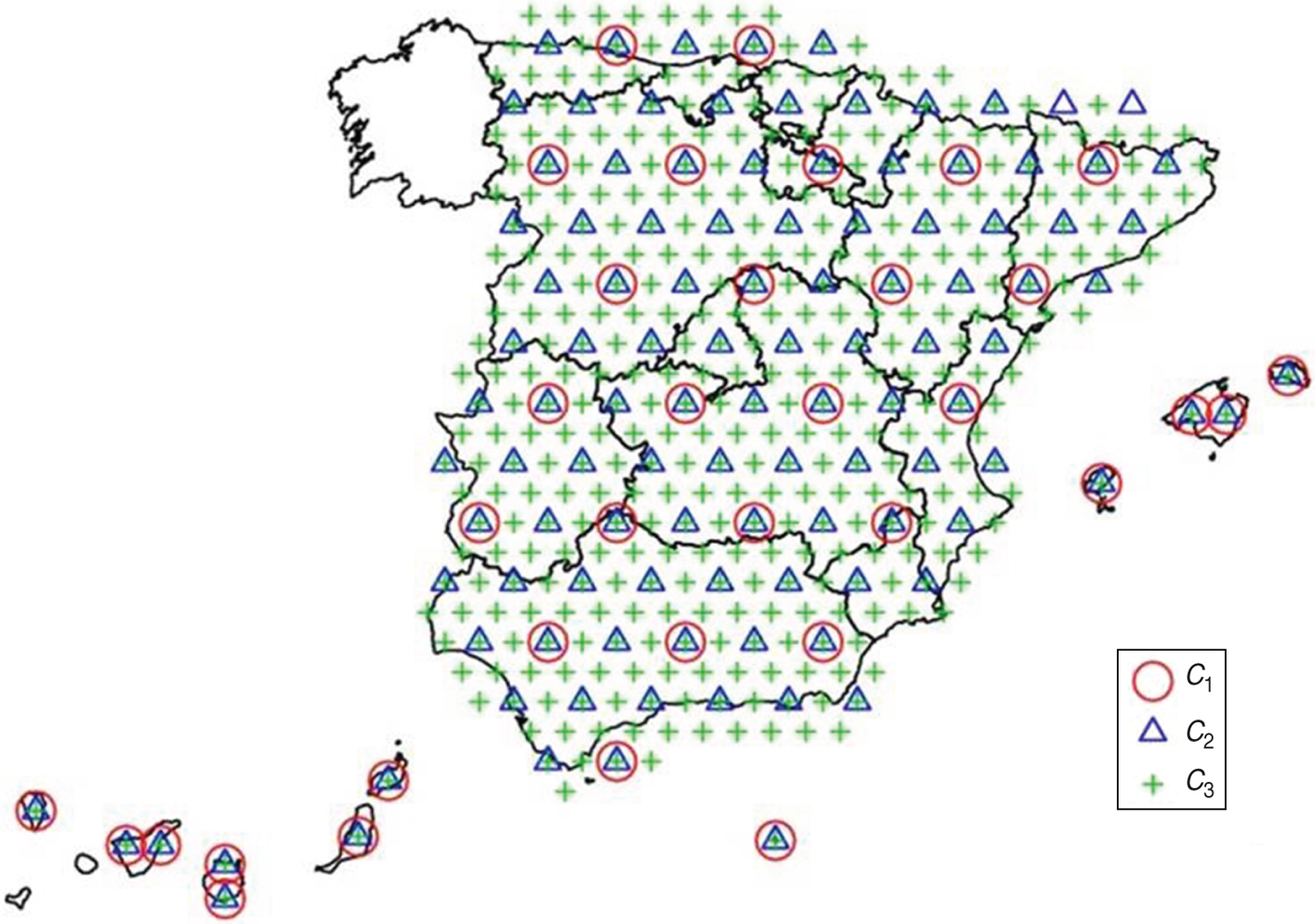
Fig. 2 [colour online]. Set of knots corresponding to each of the three kernel spatial processes.
To speed up computations we have considered the bivariate Normal distribution N 2(X i |X k ,σ) to be equal to 0 for those SPs and knots whose distance was >2 standard deviations (σ). This has allowed us to develop a sparse coding of the former model with a substantial computational improvement.
Inferences were drawn from the model using WinBUGS 1.4.3 (http://www.mrc-bsu.cam.ac.uk/bugs/). Six chains were run in parallel by means of six independent calls to WinBUGS, each one of them in a separate core of the server. Five thousand iterations were run from every chain, with the first 1000 being discarded as burn-in. Results from only one out of every 24 iterations were finally saved, therefore, the posterior sample from the Markov chain Monte Carlo contained a total of 1000 iterations. Spatial predictions and maps were made by means of R v. 2.13.1 (R Foundation, Austria) (http://www.r-project.org/) in order to further speed up computations in WinBUGS.
The model was implemented on a server with eight cores in order to run the required routines and obtain maps showing weekly influenza incidence.
RESULTS
Spatio-temporal analysis pandemic period
During the pandemic period spatio-temporal analysis of influenza activity in Spain revealed the first increases in influenza incidence rates took place in the second half of July [week 29 (2009)], in the north of mainland Spain and in the islands (results not shown). This influenza activity was associated with a predominant circulation of the 2009 A(H1N1) pandemic virus [Reference Larrauri15, Reference Larrauri17, 19], which spread progressively towards the south of mainland Spain during summer 2009 [19]. The influenza incidence maps for the beginning of September, showed increases of influenza incidence rates in most of the SISS sentinel networks [week 39 (2009)] (Fig. 3). This reflected the pandemic wave which began in Spain during weeks 39–40 (2009), and peaked at the national level at week 46 (2009). This data dovetails with ILI spread rates and other surveillance indicators. During the pandemic wave's rising phase, the influenza incidence maps showed influenza activity spreading from west to east. The highest modelled ILI rates were registered by sentinel networks in the west of mainland Spain in weeks 41–42 (2009), in the centre in week 43 (2009), and in the east in weeks 45–46 (2009).

Fig. 3 [colour online]. Spread of influenza during the pandemic period.
From week 47 (2009), the modelled ILI rates progressively declined throughout the SISS-monitored territory and, in the last weeks of surveillance, fell to very low levels nationwide, except for some specific foci.
The weekly modelled ILI rate maps (see http://vgripe.isciii.es/gripe) correspond to the entire pandemic period in Spain, as well to the following two influenza seasons.
2010–2011 season
The first increases in modelled ILI rates were observed in weeks 47–48 (2010) in the western part of mainland Spain and was seen to spread, advancing steadily eastwards [week 50 (2010)] (Fig. 4). In week 51 (2010), the upward phase of the epidemic wave started and the highest modelled ILI rates occurred in the north-west of mainland Spain. Over the following week [week 52 (2010)], influenza activity continued to rise along the north-west corridor. However, the beginning of the increases in influenza activity in those sentinel networks situated in the east and south-east of the mainland was observed in weeks 2–4 (2011). From week 6 (2011) and during the following weeks, the modelled ILI rates were observed to decline progressively throughout the country, with the epidemic wave ending at week 8 (2011) (Fig. 4). This decline started first in the north-west side of Spain, precisely the region where the epidemic wave had first arrived.

Fig. 4 [colour online]. Spread of influenza during the 2010–2011 season.
The 2010–2011 influenza epidemic wave plotted a north-west/south-east pattern of spread across mainland Spain.
2011–2012 season
During the 2011–2012 season, modelled ILI rates started to increase in weeks 50–51 (2011) (Fig. 5) in the centre of mainland Spain. In week 52 (2011), the influenza incidence rate did exceed the baseline threshold at the national level, heralding the beginning of the upward phase of the epidemic wave. Nevertheless, the spatio-temporal distribution of incidence shows a distribution of modelled ILI rates very focused at the centre of mainland Spain and influenza activity had not yet spread throughout the whole country. During the following weeks of the epidemic seasonal period the modelled ILI rates continued to be higher in the centre of the mainland with influenza activity later spreading heterogeneously across the rest of the territory. In week 6 (2012) the influenza activity began to decline progressively in the centre while in other geographical sentinel networks it was still high. From week 12 (2012) the modelled ILI rates reached pre-epidemic values across the country.

Fig. 5 [colour online]. Spread of influenza during the 2011–2012 season.
During the 2011–2012 season, the epidemic wave did not show a defined geographical pattern. The geographical propagation of the influenza activity was heterogeneous.
For each influenza season, influenza incidence maps for each surveillance week were obtained <24 h after collection of influenza surveillance data and were displayed on the SISS webpage in a timely manner during the entire influenza season.
A thorough analysis of the model for the pandemic period
Beyond the epidemiological results of the pandemic period and influenza seasons already described, some specific results of the model for the pandemic period are now presented.
Table 1 shows the variability accounted for every factor intervening in the modelling of the log-incidence (I ij in the model). Every term in Table 1 corresponds with the mean of the empirical posterior standard deviation of the random effects in the model. Higher variability corresponded to the temporal term. Heterogeneity among sentinels is the second source of variability in the study.
Table 1. Variability

s.d., Standard deviation; CI, confidence interval.
Regarding the variability of the spatio-temporal term, Table 1 indicates that the main source of variation comes from very close locations (short-range dependence or local dependence). The importance of this term is closely followed by the long-range or regional dependence and finally the medium-range term contributes far less than the other two terms to spatio-temporal variability. That is, there are two important sources of variability in the data, the first one is mainly local and the second one is mainly regional of a large range. The local term would indicate variations in incidence which are very focused in specific locations. By contrast, the regional term indicates smooth geographical differences in incidence, i.e. the epidemic wave would show marked geographical differences, e.g. causing the peak of the epidemic to be reached in some places before than in others. In any case, this decomposition of the variability shows the importance of the multi-scale approach as it allows the inclusion of different scales of dependence into the model. This desirable property cannot be easily reproduced within a geostatistical approach.
Finally, the term modelling heterogeneity between notifications (ε ɛ) has also a considerable variability. This value, of comparable magnitude to the standard deviations of the rest of the terms in the model, advises us against leaving it out of the model. This term accounts for the specific behaviour of some sentinels in some specific weeks. That is, the specific modelling of those variations is needed in order to correctly reproduce the spatio-temporal pattern of the disease.
DISCUSSION
This study analysed the spatio-temporal distribution of influenza incidence rates in the pandemic period and in the 2010–2011 and 2011–2012 influenza seasons in Spain. The estimates of influenza incidence in the territory monitored by the SISS were smooth in space and time. They displayed a coherence in spatial distribution, without any sharp increases or decreases in spatially contiguous territories. Furthermore, coherence was observed in the time trend, with no sudden, inexplicable changes from one week to the next. This is in sharp contrast to purely spatial (not spatio-temporal) models.
For the three influenza seasons analysed, the pattern of geographical progression of influenza activity was not similar. While the modelled ILI sequence rate pattern during the summer weeks of 2009 was north-south, influenza activity was seen to spread from west to east in autumn 2009. In the 2010–2011 season, the geographical spread pattern of the wave was north-west to south-east. In the 2011–2012 season, no specific geographical pattern of influenza spread could be observed. In one study analysing the trend in influenza activity in Europe over seven influenza seasons, from 2001–2002 to 2006–2007, the influenza spread activity similarly failed to display a similar pattern in the influenza seasons [Reference Paget20]. This same study described a north-south pattern of spread for three seasons and a west-east pattern for the other four, resembling the heterogeneity observed in our study for Spain in the three seasons.
Geostatistical kriging models have been previously used in several countries to study influenza incidence [Reference Abellan10, Reference Carrat and Valleron11, Reference Uphoff13, Reference Sakai21]. Recently, Inaida et al. [Reference Inaida22] analysed the geographical trend spread of pandemic (H1N1) 2009 in metropolitan areas of Japan, based on sentinel-network data. Nevertheless, one of the main advantages of our approach over traditional kriging methods is its computational convenience. For example, to run our model for the last week of season 2010–2011 we have 841 SPs*32 weeks = 26912 observed values for that same season, plus 867 SPs*52 weeks = 45084 observed values for the previous season. In that case we are jointly modelling 71 996 values in a single model, where most of these values are (spatio-temporally) dependent. This is not affordable for many methods. Both the temporally conditional formulation of the autoregressive structure and the computational convenience of the kernel processes have made it possible to carry out inference in our setting.
The methodology proposed in this paper follows the model already developed by Martinez-Beneito et al. [Reference Martinez-Beneito, Botella-Rocamora and Zurriaga14]. Nevertheless, our model has one novelty with respect to the former proposal. We have resorted to several kernel processes of different ranges in order to describe the spatial dependence. This has been possible as the amount of data we have available in our system makes it feasible to include different kernel processes and to determine which of them should have a higher contribution to explain the data under the model setup. The process resulting from this new multi-resolution approach can be viewed as a mixture of spatial patterns of different ranges. This yields a broader class of spatial processes as it can accommodate several patterns of different range (and therefore of different nature) in a single proposal.
There are other studies in different countries during the pandemic period that used spatial and temporal analysis of influenza. For instance Chowell et al. [Reference Chowell23] analysed the spatial distribution of A(H1N1)pdm09 influenza in Peru during this period. To show the maps of the distribution of the disease these authors used ILI data and represented the cumulative number of cases for provinces and the peak day for spatial unit. Their results showed substantial spatial variability in the pandemic pattern across the country. The same authors [Reference Chowell24] analysed influenza surveillance data to made a spatial and temporal analysis during the pandemic, concluding that there were three spatially heterogeneous waves of the A(H1N1)pdm09 in Mexico. Our study shows that Spain experienced a pandemic wave in autumn 2009, in line with other indicators of influenza activity.
We have also analysed the spatio-temporal diffusion of influenza in the following two seasons. In our study the temporal term is the most important source of variability. This is not surprising since it is very unlikely to obtain high influenza incidence values for non-epidemic periods and vice versa. That is, time was expected to be one of the main determinants of influenza incidence, which has been confirmed with our analysis.
In addition, another reported limitation of geographical studies of influenza incidence which rely on sentinel networks, is the difference in sensitivity of participating SPs when it comes to deciding whether or not a patient seeking attention suffers from influenza symptoms [Reference Uphoff13]. Some authors have tried to control for heterogeneity in SP reporting, by using harmonization indices for consultation to study trends in influenza incidence in Germany and Holland [Reference Uphoff13]. Allowance is made for this factor in the spatio-temporal model applied in this study [Reference Martinez-Beneito, Botella-Rocamora and Zurriaga14], i.e. by including a term to control for the dynamic of each SP's over- or underreporting which takes each SP's seasonal behaviour into account, thereby reducing the bias in incidence estimates. We confirm in this study that heterogeneity among sentinels is the second source of variability. This makes it absolutely necessary to control for this term within the model if we want to produce accurate estimates of the geographical spread of disease. Otherwise, without controlling for this term, the geographical pattern would show persistent spurious peaks caused by the presence of abnormal sentinels at some specific places.
Regarding the spatio-temporal term, there are two important sources of variability in the data, the first is mainly local (short range) and the second is mainly regional (long range). The local term would indicate variations in incidence which are very focused in some specific locations. By contrast, the regional term indicates smooth geographical differences in incidence, i.e. the epidemic wave would show marked geographical differences, e.g. causing the peak of the epidemic to be reached in some places before others. In any case, this decomposition of the variability shows the advantage of the multi-scale approach as it allows the inclusion of different scales of dependence into the model.
Finally, the term modelling heterogeneity between notifications (ε ɛ) has also a considerable variability. This value, of comparable magnitude to the standard deviations of the rest of terms in the model, advises us against leaving it out of the model. This term accounts for the specific behaviour of some sentinels in some specific weeks. That is, the specific modelling of those variations is needed in order to correctly reproduce the spatio-temporal pattern of the disease.
In spite of the factors mentioned, we cannot exclude other factors that can influence the morbidity-related site effect independently of the behaviour of the SP. Thus, despite controlling for heterogeneity in SP reporting, there are still areas or sentinel networks where influenza incidence remains systematically higher than elsewhere after the seasonal wave has ended. This suggests that other factors relating to uniformity of influenza case-reporting criteria in the different sentinel networks may be influencing the geographical estimates made. Indeed, a SISS assessment study [Reference Negro25] revealed a great degree of heterogeneity in the use of the influenza case-definition by different sentinel networks. New assessment studies are thus required, especially following the reinforcement of SISS activity during the 2009 pandemic, in order to achieve greater harmonization in surveillance criteria and systematic data collection in all the sentinel networks comprising the SISS.
We used the weekly ILI rates of each SP as a marker of influenza activity, since this was the parameter available for inclusion of each SP in the model. Other indicators of influenza activity could be virological, as the percentage of positive specimens, or a mix indicator which would take in account clinical and virological information. Further approaches considering the use of other markers of influenza activity, including variation by age and type/subtype of influenza virus, are ongoing to monitor the spatio-temporal spread of the influenza in Spain.
Another limitation of this study stems from the fact that our analysis did not include information on the entire mainland area, as two ARs had no sentinel networks. Furthermore, in ‘frontier’ areas, such as those bordering on either of the ARs for which no information is available, or having natural or administrative boundaries with other countries, there is a ‘so-called’ edge or boundary effect [Reference Pfeiffer26], which consists of obtaining less precise estimates.
Using the influenza incidence maps obtained in this study, the spread of influenza epidemic waves can be displayed and analysed at both national and regional levels, and foci of high influenza incidence eligible for adoption of disease-control measures can be identified. Starting with influenza season 2010–2011, the model of spatio-temporal spread of influenza incidence was implemented in the SISS as a supplementary tool of influenza surveillance in Spain. This map was obtained with a short delay, <24 h, and it has great spatial disaggregation. This is possible because of the existing coordination between the SISS sentinel networks and reception and analysis of the data.
As a result, geographical national and regional maps of influenza incidence in Spain have been disseminating weekly via the SISS webpage (http://vgripe.isciii.es/gripe/inicio.do).
APPENDIX Members of the Scientific Committee of Project GR09/020 (Development and implementation of a methodology for estimating the maps of influenza incidence from sentinel networks using a mixed Poisson regression Bayesian model)
Diana Gómez, Amparo Larrauri, Silvia Jiménez, Fernando Simón, Victor Flores, Inmaculada León (Centro Nacional de Epidemiologia, ISCIII); Miguel Angel Martínez-Beneito (Centro Superior de Investigación en Salud Pública); Paloma Botella (Universidad CEU-Cardenal Herrera); Oscar Zurriaga, Maite Miralles, Aurora López Maside (Área de Epidemiología, Dirección General de Salud Pública de la Generalitat Valenciana); Representatives of the Spanish influenza sentinel networks: Esteban Perez, Elisa Rodríguez Romero (Servicio de Epidemiología y Salud Laboral, Consejería de Salud de la Junta de Andalucía). Silvia Martínez Cuenca (Servicio de Vigilancia en Salud Pública, Dirección General de Salud Pública de Aragón); Maria del Pilar Alonso Vigil (Dirección General de Salud Pública y Participación, Consejería de salud y servicios sanitarios, Asturias); Jaume Giménez (Servei d'Epidemiologia, D.G. Salut Pública i Participació, Govern de les Illes Balears); Lucas Gonzalez (Servicio de Epidemiología y Prevención, Consejería de Sanidad, Canarias); Sergio Gutierrez Gonzalez (Dirección General de Salud Pública, Consejería de Sanidad del Gobierno de Cantabria); María Victoria García Rivera (Servicio de Epidemiología, Consejería de Sanidad de Castilla la Mancha); Sonia Tamames, José Eugenio Lozano Alonso (Dirección General de Salud Pública e I + D + I. Consejería de Sanidad Junta de Castilla y León); Luca Basile (Subdirecció General de Vigilancia i Resposta a Emergències en Salut Pública, Departament de Salut, Generalitat de Catalunya); Ma del Carmen Serrano Martin, Julián Mauro Ramos Aceitero (Dirección General de Salud Pública, Consejería de Sanidad y Dependencia de la Junta de Extremadura); Soledad Cañellas Llabrés, Ana Gandarillas (Dirección General de Atención Primaria de la Consejería de Sanidad de la Comunidad de Madrid); Jesús Castilla (Sección de Vigilancia de Enfermedades Transmisibles, Instituto de Salud Pública de Navarra); Miguel Ángel García Calabuig (Epidemiología e Información Sanitaria de la Dirección de Salud Pública del País Vasco); Carmen Quiñones, Milagros Perucha (Sección de Vigilancia Epidemiológica y Control de Enfermedades Transmisibles, La Rioja); Ana Rivas (Servicio de Epidemiología, Consejería de Sanidad y Consumo, Ceuta); Daniel Castrillejo Pérez (Dirección General de Sanidad y Consumo, Melilla).
ACKNOWLEDGEMENTS
The authors are grateful to the sentinel physicians and all professionals participating in the Spanish Influenza Surveillance System. This work was supported by the Research Program for Influenza A(H1N1)pdm09 of the Institute of Health Carlos III (GR09/020).
DECLARATION OF INTEREST
None.


