


INTRODUCTION
Rubella is primarily a mild childhood disease, but acquiring the infection during the first 16 weeks of pregnancy is associated with the risk of fetal death or birth of a child with congenital rubella syndrome (CRS). CRS is a condition associated with a range of problems, from hearing impairment to brain damage. Estimates of the burden of CRS are high in many developing countries [Reference Cutts and Vynnycky1] and may frequently go unreported [Reference Lawn2]. Since vaccination drives up the average age of infection, increasing the proportion of women of child-bearing age at risk [Reference Knox3–Reference Massad7], many countries in the developing world are not vaccinating against rubella [Reference Robertson8], particularly given recent work indicating how partial vaccination of populations can increase the population-wide risk of CRS by allowing build-up of susceptible individuals in older age groups [Reference Vynnycky, Gay and Cutts9]. Multi-annual outbreak cycles are another factor that may allow such build-up because the deepened post-epidemic troughs may lead to local extinction and periods of lowered force of infection [Reference Ferrari10, Reference Metcalf11].
Across much of the developing world, recent efforts to reduce the burden of measles mortality [Reference Wolfson12] via measles vaccination campaigns has lead to an increase in national vaccination coverage capacity and second-dose availability. In this context, it is of interest to revisit the risks associated with introduction of the rubella vaccine [Reference Plotkin13]. A major challenge to quantifying the potential CRS burden is that details of the drivers of rubella dynamics remain unclear. Where rubella dynamics have been described, multi-annual cycles of varying periodicity are generally observed [Reference Anderson and May14] and competing explanatory mechanisms have been put forward (summarized in Table 1). Depending on the particular mechanism underlying multi-annual cycles, vaccination might either increase or decrease the period between major epidemics by shifting dynamics between multi-annual and annual regimens. Identifying both whether rubella dynamics are multi-annual, and if so, the mechanism underlying such multi-annual epidemics is therefore of programmatic interest. The mechanisms hypothesized hang on the treatment of seasonal patterns of transmission (Table 1), currently generally assumed to reflect term-time forcing, i.e. increases in transmission associated with aggregation of children in schools, and decreases during vacations [Reference Fine and Clarkson15]. However, whether this assumption is valid is unclear, since estimation of seasonal variation of transmission from time-series has been rare, and estimates from countries outside Europe and North America are non-existent. There is also as yet very little information on the critical community size (CCS) of rubella, i.e. the population size required for the infection to persist locally without stochastic extinction [Reference Bartlett16].
Table 1. Different mechanisms proposed to explain multi-annual cycles in childhood infections
The ideal dataset to tackle these questions would be spatio-temporal time-series of incidence for rubella, coupled with information on the age structure of incidence. Data on rubella are relatively rare compared to those on measles because it is a milder disease which is somewhat harder to diagnose. The notification record from Mexico coordinated by the Dirección General de Epidemiología of the Mexican Ministry of Health (described in [Reference Vargas17]) provides an excellent opportunity to explore rubella dynamics. Rubella has been a reportable disease in Mexico since 1985 and vaccination against rubella with the MMR vaccine was implemented in 1998 as part of a broader Pan-American Health Organisation (PAHO) effort, which successfully reduced incidence to very low levels [Reference Santos18].
Here we use district-level monthly data from Mexico from 1985 to 2007 and yearly data on age structure to explore the critical dynamical questions. We first estimate some basic parameters of the epidemiology of rubella in Mexico to compare with results from other countries [Reference Cutts and Vynnycky1] and explore regional patterns of extinction (‘fade-out’) to establish whether stochastic dynamics are likely to be important. We then use spectral analysis to explore the magnitude of multi-annuality in the dynamics, and explore whether this can be attributed to transient dynamics [Reference Bauch and Earn19]. We fit a time-series Susceptible–Infected–Recovered (TSIR) model to estimate seasonal swings in transmission [Reference Bjørnstad, Finkenstadt and Grenfell20]. With this, we finally explore the determinants of patterns of seasonality, and whether these vary by district size or socioeconomic characteristics. We discuss the implications of our results for identifying populations most at risk for CRS and for the implementation of vaccination campaigns.
METHODS
The data
Rubella incidence reports were obtained from ref. [21]. Monthly reported cases between 1985 and 2007 were available for each of the 32 states of Mexico (Fig. 1), at the spatial scale of districts. For 1990–2007, district-level yearly incidence is available in age groups of 5–10 years (e.g. 1–4, 5–14, 15–24, etc.). The MMR vaccine was introduced in 1998 and resulted in relatively high coverage [Reference Santos18]. Birth numbers and population size for each district in each month were obtained from ref. [22]; as were socioeconomic indicators of each of the districts.
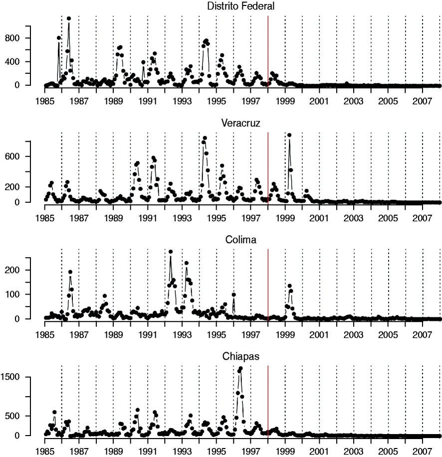
Fig. 1. Time-series of rubella from four districts in Mexico, representing a range of population size (see Table 2); the year at the start of vaccination is shown by a red vertical line.
Average age of infection and R 0 from the age-structured data
Assuming negligible mortality in the disease-relevant age groups and a constant force of infection, the mean age of infection A is defined by A=∫xσ(x)dx, where x is age and σ(x) is the proportion susceptible at age x. From this, using 1−[the cumulative proportion of case numbers over age] as a proxy for the proportion susceptible in each discrete age group, we calculated A for each district, and explored spatial patterns of average age of infection. This estimate of the average age of infection can also be used to obtain a crude estimate of the basic reproduction number, R 0, for every district. In a growing population, A is related to R 0 by R 0~G/A where G is the inverse of the per capita birth rate [Reference McLean and Anderson23], here set to the inverse of the mean birth rate of each district. The value of R 0 estimated in this way may be biased by a range of factors, particularly differences in the force of infection over age [Reference Farrington, Kanaan and Gay24]. Nevertheless, the relative magnitude of R 0 across districts should remain comparable, as long as district-specific differences in the force of infection over age are not too great. To verify this, we fitted a logistic regression to the cumulative proportion of cases over age across the entire dataset, with age fitted as a continuous covariate and district fitted as a factor. Significant variability attributable to district in the profile of infection over age would imply that transmission varies over age such that the average age is a poor indicator of the relative magnitude of R 0.
Critical community size
Since population size is a key determinant of stochastic extinction for strongly immunizing infections, population size is strongly negatively related with the number of fade-outs (or proportion of zeros) in the time-series of incidence [Reference Bartlett16, Reference Bjørnstad, Finkenstadt and Grenfell20]. The point where this curve intercepts with zero provides an indication of the CCS, or population size below which the infection is subject to stochastic fade-outs. Since under-reporting could lead to apparent fade-outs where there are none [Reference Bartlett16], we define fade-outs as corresponding to a full month with zero reported cases. Since case reporting is at the district level, rather than the city level, and since cities are more likely to be the epidemiologically relevant unit, this estimate is likely to be an upper bound on the CCS.
Spectral analysis
To test whether predicted relationships between population size and periodic features of the time-series were upheld (Table 1) we calculated periodograms of the rubella time-series for each district using modified Daniell smoothers of width 2 [Reference Venables and Ripley25]. We located the main peaks in spectral density and identified the multi-annual peak with a period closest to an integer multiple of a year as ‘resonant’ [Reference Bauch and Earn19]. For six time-series, only a single peak could be identified. For the remaining 26 districts, we tested for correlations between population size and the ratio between the resonant and the second largest peak (‘non-resonant peak’) [Reference Bauch and Earn19]. If stochastically excited transients are a driver of multi-annuality this ratio should decrease with populations size (Table 1).
The TSIR model
Seasonal transmission rates can be estimated using TSIR methods [Reference Bjørnstad, Finkenstadt and Grenfell20] in a Bayesian state-space framework [Reference Ferrari26]. The generation time (serial interval) of rubella (approximately the latent plus infectious period) is ~18 days [Reference Anderson and May14], so we assumed that the time-scale of the epidemic process was approximately 2 weeks, resulting in two unobserved epidemic time-steps for each observed monthly report (repeating the analysis taking a monthly time-step does not alter the major conclusions). Denoting Y m as the number of cases reported in month m, and I m the unobserved total number of cases, the observation process is defined by Y m~binomial(I m, p obs ), where p obs is the reporting rate. The unobserved epidemic follows the TSIR process model where the number of infected individuals at time t+1, I t+1 depends stochastically on I t, and the number of susceptible individuals S t, with expectation λt+1=βmS tI tα/N t, where βm is the transmission rate in every month and the exponent α, usually a little less than 1, captures heterogeneities in mixing not directly modelled by the seasonality [Reference Bjørnstad, Finkenstadt and Grenfell20, Reference Finkenstadt and Grenfell27] and the effects of discretization of the underlying continuous time process [Reference Glass, Xia and Grenfell28]. Note that inasmuch as the time-step used represents the true average time from infection to recovery, βm estimated in this way corresponds to the seasonally varying basic reproductive number R 0 (since it indicates the number of new infections caused by a single infected individual in a wholly susceptible population), and thus the median value of βm can be compared to estimates of R 0 obtained using age-based calculations. We model I t+1 as a negative binomial random variable with expectation λt and clumping parameter I t [Reference Bjørnstad, Finkenstadt and Grenfell20]. Susceptible individuals are depleted by infections and replenished by births, B t, and are modelled with the renewal equation S t+1=S t +B t−I t+1. Since vaccine coverage levels are thought to be around 80%, and vaccinated individuals avoid susceptibility, births are discounted by 0·8 following the start of vaccination (i.e. post-vaccination, S t+1=S t+0·2B t−I t+1). We assumed that infection predominantly occurs early in life, so that depletion of susceptible individuals by mortality can be neglected.
We used a Bayesian state-space model to obtain parameter estimates. Flat priors were set on the number of susceptible individuals at every time-step, with the upper and lower limits set to constrain the time-series to reflect a 20% range around the known proportion of susceptible individuals in 1990 [Reference Trujillo, Munoz and Tapia-Conyer29]. Uninformative priors were set for the βm parameters (a normal distribution left-truncated at zero with a mean of 6 and a standard deviation of 10); and flat priors were set on the α parameter, constraining it to be between 0·9 and 1. We set an informed prior on the observation probability p obs, centred at an initial estimate obtained from susceptible reconstruction [Reference Bjørnstad, Finkenstadt and Grenfell20, Reference Finkenstadt and Grenfell27] for each district, following a beta distribution to allow for direct sampling.
We initiated the chain with constant monthly transmission set to 6, and α=0·95. At each iteration, we chose at random to update candidates of either one of the βm parameters or the α parameter, or a subset of the unobserved process, I t, also chosen at random. If the latter was chosen, we used the renewal equation to obtain the corresponding numbers of susceptible individuals through time, and checked that this violated none of the conditions or priors. If the candidate proved suitable, we then calculated the acceptance ratio for the candidate parameters (calculated by the product of the likelihood of the observation model, the likelihood of the process model and the prior density functions of the candidates, divided by the same three elements as calculated for the current parameter values). We accepted or rejected the candidates accordingly, and then used a Gibbs step to update observation probabilities. After a burn-in of 10 000 iterations we ran the chain for 100 000 iterations, sampling every 100th step to avoid autocorrelation.
RESULTS
Age of infection
The mean age of infection estimated for the pre-vaccination era (before 1999, see above) ranges between 3 (Zacatecas) and 11 (Veracruz) years, with highest average ages of infection concentrated in the south and coastal areas of the country (Fig. 2); age-based R 0 estimates are correspondingly low in these locations (Table 2). A logistic regression relating the cumulative proportion of infected individuals over age showed no significant effect of location (χ312=2·92, P>0·5, Fig. 3), suggesting that the relative magnitudes of R 0 estimated in this way are comparable across locations (although episodic dynamics will provide a further slight bias, see below).
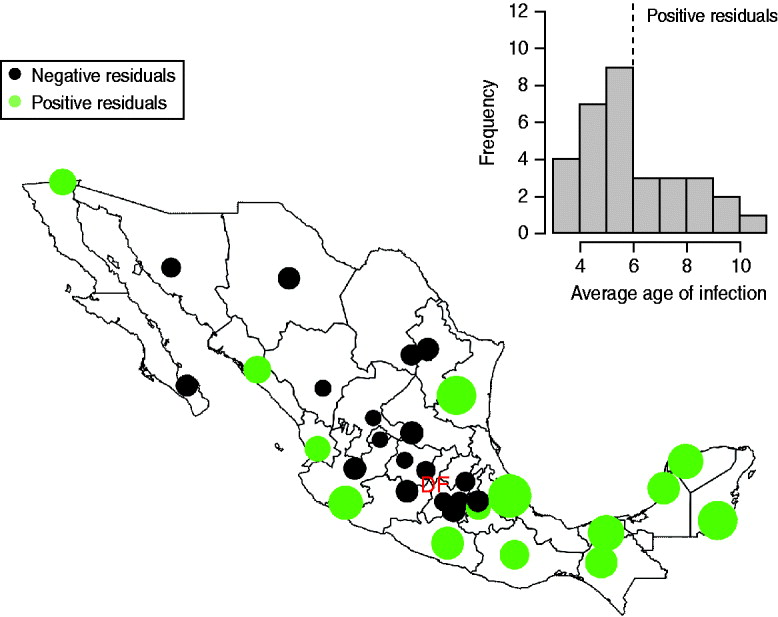
Fig. 2. The inset shows a histogram of average age at infection taken from years before 1999; the dotted vertical line indicates the countrywide average. The map shows the magnitude (point size) and sign of deviations from the countrywide average log age of infection (point colour) taken from this inset histogram. Points are placed in district capitals. Districts centred around the district containing the capital city (‘Federal District’ indicated as ‘DF’) have a lower than average age of infection; coastal and southern districts have a higher average age of infection.
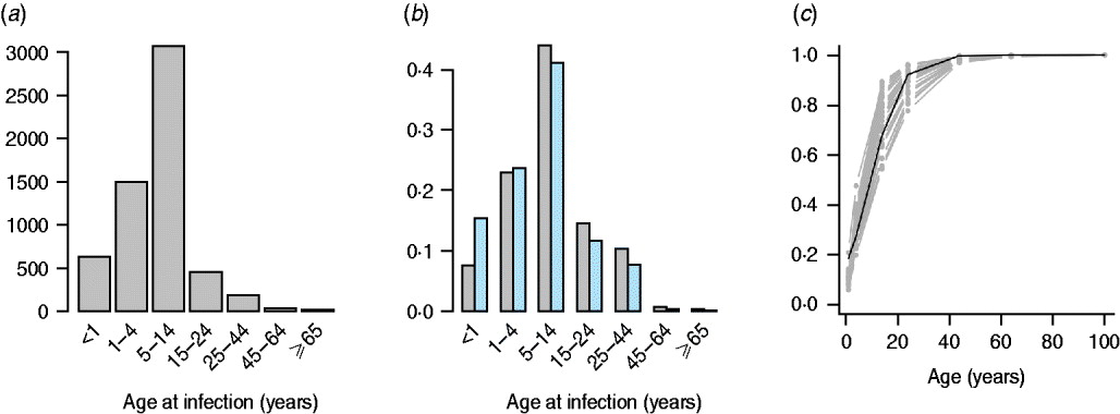
Fig. 3. The pattern of infected individuals across age showing (a) numbers reported from 1985 to 1999 across the whole of Mexico; (b) the proportion across age from 1985 to 1999 in the smallest (Baja California Sur) and largest (Federal District) districts, similar profiles are obtained in all other districts; and (c) the cumulative proportion over age (grey lines) and a logistic regression fitted to this data [black line, logit(y) ~−1·67(0·33)+0·17(0·02)×age, χ12=7·72, d.f.=223, P<0·01; parentheses indicate standard errors]. Incorporating district as a factor did not significantly improve this model (χ312=2·92, P>0·5), suggesting little regional difference in the pattern of force of infection over age.
Table 2. Average age at infection, median transmission rate estimated from the TSIR analyses, β, and the corresponding estimated reporting rate, pobs, and heterogeneity parameter, α (see text); with R0 estimated from the age data for each district, and the district's rank by population size (the range of population sizes are shown in Fig. 4)
Average age of infection was not significantly related to population size (F 1,30=0·20, P>0·5), or districts' socioeconomic indicators (F 1,30=3·51, P>0·05). Estimates of average age of infection are consistent with global patterns of results on seronegativity, which generally indicate that more than half of the population has been infected by age 13 years [Reference Cutts and Vynnycky1]; estimates are also in line with the incidence-based estimate of an average age of infection of approximately 9 years from Peru [Reference Metcalf11].
Critical community size
The relationship between proportion of zero incidence and log population size in the pre-vaccination era is very noisy, and more triangular than linear. However, the relationship is significantly negative (F 1,30=8·61, P<0·01), and provides an indicator of the order of magnitude of the CCS as being larger than a million (Fig. 4). This is comparable to estimates from Peru [Reference Rios-Doria and Chowell30].
Fig. 4. The relationship between log population size and proportion of zeros in the time-series for years up to 1998 when vaccination was started (Fig. 1). The dashed line is y=0·154–0·009x, P<0·01, r 2=0·22. The line intersects zero at a population size of 8 500 000; no occurrence of zero fade-outs occurred in districts smaller than one million.
Spectral analysis
Across districts, the mean period of the non-resonant peak was 3·79 years with a standard deviation of 1·25 years. The resonant peak was 1 year for all districts, and the magnitude of the non-resonant peak was greater than the resonant peak in only three districts (Baja California Sur, Quintana Roo, Tabasco). Two of these are the smallest populations in the data. The relationship between population size and the ratio of the magnitude of the resonant and non-resonant peaks, denoted k, was significant (Fig. 5), supporting the role of stochasticity in driving inter-annual variability (Table 1) via transient dynamics [Reference Bauch and Earn19]. Log average age of infection was also significantly and positively related to the ratio of the magnitude of the resonant and non-resonant peaks (F 1,25=10·41, P<0·05, r 2=0·22, with y=4·74+2·00k), i.e. districts with more strength in the non-resonant peak had a higher average age at infection. This suggests that stochasticity may increase the mean age of infection (and may slightly bias estimates of R 0 obtained above). Including the mean transmission rate β estimated via the TSIR (see below) did not significantly improve this regression model (F 1,24=0·06, P>0·4).
Fig. 5. Spectral density of log reported rubella incidence +1 for two districts in Mexico, with the resonant and non-resonant peaks shown as vertical dashed lines; and the ratio of the non-resonant peak over the resonant peak across population size for districts where the non-resonant peak was identifiable (26/32 districts). Point size scales inversely with the precision of the second peak (large points correspond to sharp peaks, small points correspond to broad peaks). The equation of the line is y=3·49–0·21x, P<0·01, r 2=0·26, and corresponds to a regression weighted by the precision of the second peak (the unweighted regression is also significant).
Seasonality and transmission magnitude
The overall magnitude of seasonal transmission estimated via the TSIR model (which can be equated with R 0, see above) concurred with the broad estimate of R 0 obtained via average age of infection (Table 2), suggesting relatively low transmission in this infection relative to the most contagious childhood infections such as whooping cough or measles [Reference Anderson and May14]. Seasonal variation in transmission rates estimated by the Bayesian state-space TSIR showed a signal of term-time forcing, with low transmission in July; this pattern did not vary much across socioeconomic indicators (Fig. 6). The coefficient of variation in seasonality of transmission ranged from 0·16 (Oaxaca) to 8·57 (Durango). There were no clear geographical differences in the pattern of seasonality (not shown) and no correlation between magnitude of seasonality and socioeconomic indicators (n=32, ρ=−0·20, P>0·1). The coefficient of variation of seasonality and the average age of infection were significantly negatively correlated (n=32, ρ=−0·37, P<0·05), so that locations with higher amplitude transmission also had a lower average age of infection.
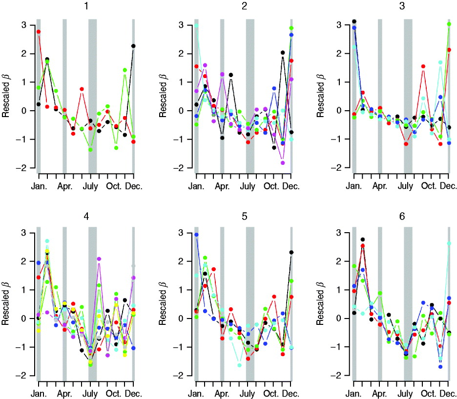
Fig. 6. Pattern of seasonal transmission rates across districts, organized according to the socioeconomic status rankings (see Methods section): ‘1’ indicates low, and ‘6’ indicates high. Transmission rates have been scaled to have the same mean and variance to facilitate comparison of seasonality. Colors are (1) Chiapas=black, Guerrero=red, Oaxaca=green; (2) Campeche=black, Hidalgo=red, Puebla=green, San Luis Potosi=blue, Tabasco=turquoise, Veracruz=pink; (3) Durango=black, Guanajuato=red, Michoacan=green, Tlaxcala=blue, Zacatecas=pink; (4) Colima=black, Mexico=red, Morelos=green, Nayarit=blue, Queretaro=turquoise, Quintana Roo=pink, Sinaloa=yellow, Yucatan=grey; (5) Baja California=black, Baja California Sur=red, Chihuahua=green, Sonora=blue, Tamaulipas=turquoise; (6) Aguascalientes=black, Coahuila=red, Jalisco=green, and Nuevo Leon=blue, Distrito Federal=turquoise. Approximate school holidays are shown in grey (2 weeks at Christmas, 2 weeks at Easter, and July to mid-August).
DISCUSSION
Our results point to considerable regional variability both in patterns of seasonality and average age of infection of rubella across Mexico, with for example low average age of infection around Mexico City (in agreement with a previous serosurvey in this district [Reference Golubjatnikov, Elsea and Leppla31]), and higher average age of infection in the southern and coastal regions (Fig. 2). This variation in the average age of infection could result from either regional variability in R 0, or regional variability in the importance of episodic dynamics, as Ferrari et al. [Reference Ferrari10] have demonstrated that such dynamics can inflate the upper tail of the age-incidence curve. Various lines of evidence support the latter explanation (see below). Our results also indicate some general patterns for the epidemiology of rubella in Mexico such as a signal of term-time forcing [Reference Fine and Clarkson15] with lower transmission during school holidays found across the country (Fig. 6), as has also been indicated by a recent analysis of rubella in Peru [Reference Metcalf11, Reference Rios-Doria and Chowell30].
Our results provide general support for stochasticity as a driver of rubella dynamics. Our analysis suggests a CCS for rubella larger than 1 000 000, considerably larger than the estimate for measles in the UK, estimated to be between 300 000 and 500 000 [Reference Bartlett16]. This figure is likely to be an overestimate since the geographic unit used is districts rather than cities, but the large CCS is not unexpected given the comparatively weaker transmission rate of rubella relative to measles, and is consistent with one other estimate for rubella in Peru [Reference Rios-Doria and Chowell30]. This suggests that local extinction is likely to be frequent, inducing more episodic dynamics and allowing build-up of susceptible individuals in later age groups [Reference Ferrari10], implying that connectivity between population centres is a key direction of research in establishing the burden of CRS [Reference Metcalf11].
In contrast to the multi-annual dynamics observed for rubella in the pre-vaccination era in a range of developed country contexts [Reference Anderson and May14, Reference Bauch and Earn19], dynamics of rubella in Mexico were predominantly annual (i.e. in Figure 5, the ratio is very rarely >1, indicating that the annual resonant peak dominates). This could reflect the scale of our observation, i.e. district-level observations could be averaging highly erratic local dynamics, as in the case of measles in Niger, where country-level dynamics appear annual, but dynamics at the local scale are near-chaotic [Reference Ferrari26]. However, a discernible non-resonant peak was detectable for all but six districts, and the relative magnitude of the district-level non-resonant and resonant peaks was significantly related to the district average age of infection. This relationship with average age of infection is not predicted if local dynamics deviate from district-level observations, but is expected if local dynamics within a district are synchronized and episodic [Reference Metcalf11].
Since dynamic features do significantly correlate with the average age of infection (even though the annual features dominate), the mechanism underlying episodic dynamics remains a question of considerable interest in the context of rubella. Our results support a role for stochasticity [Reference Bauch and Earn19]; and in fact the low magnitude of the non-resonant peak relative to the resonant peak would be expected in the context of this mechanism given the relatively high population densities across districts in Mexico. This mechanism is also supported by results including (i) the relationship between population size and relative magnitude of the resonant and non-resonant peaks (Fig. 5); and (ii) estimates of R 0 which are sufficiently low (~6) as to be unlikely to drive complex multi-annual cycles alone [Reference Earn32], unless birth rates are much higher than those observed in Mexico. This importance of stochasticity in determining the dynamics of rubella is of public health significance because it provides a second mechanism by which moderate vaccination cover can enhance CRS risk; vaccination will break local chains of transmission and thus increase stochasticity in dynamics, potentially exacerbating the predicted increase in mean age relative to less stochastic settings [Reference Metcalf11].
The generality of the importance of stochasticity in rubella dynamics is an interesting question for future research. Serology data from Gabon have suggested R 0 values as high as 16 [Reference Anderson and May14], and similar magnitudes have been reported for Ethiopia and China [Reference Vynnycky, Gay and Cutts9]. Such robust transmission would considerably reduce the importance of stochasticity. Distinguishing whether deterministic high transmission or transient dynamics and fade-outs are the norm for rubella is important in considering implementation of vaccination strategies. For example, in Mexico spatially explicit deterministic models that ignore demographic stochasticity and local heterogeneities (Fig. 2) will not accurately represent disease dynamics by failing to capture frequent local extinctions, or inter-annual variability, and attempts to model optimal vaccination strategies may consequently go awry. Overall, the relatively low estimates of R 0 obtained here (Table 2), and a short generation time indicate that interrupting rubella transmission may be relatively straightforward, and this is supported by the success of the Mexican vaccination campaign (Fig. 1). However, in rubella, unless vaccination is maintained at high levels, local extinction may be followed by increases in CRS incidence resulting from the build-up of susceptible individuals in older age groups [Reference Metcalf11].
ACKNOWLEDGEMENTS
We thank the staff of Dirección General de Epidemiología and the Mexican National Surveillance System for their efforts in conducting surveillance activities and providing the rubella data used in this study. This work was funded by the Bill and Melinda Gates Foundation and grant NIH R01 GM083983-01 (C.J.E.M., B.T.G., O.N.B, M.J.F.), and the RAPIDD program of the Science & Technology Directorate, Department of Homeland Security and the Fogarty International Center, National Institutes of Health (B.T.G., O.N.B, M.J.F.).
DECLARATION OF INTEREST
None.


