


1. INTRODUCTION
Snow avalanche long-term forecasting is generally carried out on the basis of high-magnitude events defined by their return period, for example, Salm and others (Reference Salm, Burkard and Gubler1990). Such purely hazard-oriented approaches do not explicitly consider elements at risk (buildings, people inside, etc.), and neglect possible budgetary constraints. Therefore, they do not guarantee that unacceptable exposition levels and/or unacceptable costs cannot be reached. This is well demonstrated in Favier and others (Reference Favier, Eckert, Bertrand and Naaim2014b) by confronting standard hazard zone limits with acceptable risk levels as defined by Jónasson and others (Reference Jónasson, Sigurðsson and Arnalds1999). To overcome these limitations, risk-based zoning methods (Keylock and others, Reference Keylock, McClung and Magnusson1999; Arnalds and others, Reference Arnalds, Jonasson and Sigurdsson2004) and cost-benefit analyses (Fuchs and others, Reference Fuchs, Thoeni, McAlpin, Gruber and Bründl2007) have emerged recently, allowing socio-economic considerations to be included (Bründl and others, Reference Bründl, Romang, Bishof and Rheinberger2009) in a proper mathematical framework (Eckert and others, Reference Eckert2012).
Risk quantification requires, combining the model for avalanche hazard with a quantitative assessment of consequences. The hazard distribution is (at least partially) site-specific, and two main approaches exist to determine it. ‘Direct’ statistical inference can be used to fit explicit probability distributions on avalanche data, mainly runout distances (Lied and Bakkehoi, Reference Lied and Bakkehoi1980; Eckert and others, Reference Eckert, Parent and Richard2007; Gauer and others, Reference Gauer, Kronholm, Lied, Kristensen and Bakkehøi2010). As an alternative, statistical-dynamical approaches include hydrodynamical modelling within the probabilistic framework (Barbolini and others, Reference Barbolini, Natale and Savi2002; Meunier and Ancey, Reference Meunier and Ancey2004; Eckert and others, Reference Eckert, Parent, Faug and Naaim2008). They lead the joint distribution of all variables of interest, including that of spatio-temporal pressure fields (Eckert and others, Reference Eckert, Naaim and Parent2010b). Consequences for elements at risk are estimated using vulnerability relations. Vulnerability curves are increasing curves with values of [0, 1] quantifying the expected damage as a function of the avalanche intensity. Avalanche intensity is generally expressed in terms of impact pressure, but sometimes also of flow depth or velocity (Barbolini and others, Reference Barbolini, Cappabianca and Savi2004a, Reference Barbolini, Cappabianca, Sailer and Brebbiab). Existing vulnerability to snow avalanche relations has historically been assessed by back-analysis of well-documented events (Keylock and Barbolini, Reference Keylock and Barbolini2001; Papathoma-Köhle and others, Reference Papathoma-Köhle, Kappes, Keiler and Glade2010), but numerical approaches have emerged recently (Bertrand and others, Reference Bertrand, Naaim and Brun2010; Favier and others, Reference Favier, Bertrand, Eckert and Naaim2014a).
To minimise the residual risk after the construction of a defense structure, effects of such structures on avalanche flows must also be quantified. Semi-empirical analytic equations could be developed to describe the runout shortening caused by dam-like obstacles, refered to as interaction laws throughout the text in accordance with the literature (Faug and others, Reference Faug, Naaim, Bertrand, Lachamp and Naaim-Bouvet2003) They have been established for walls spanning the whole width of the incoming flow with the help of theoretical arguments combined with small-scale laboratory tests on granular avalanches. Specifically, two existing interaction laws correspond to idealised situations for which the runout shortening is caused by either the local dissipation of kinetic energy (purely inertial regime) or the volume reduction due to storage of the snow upstream of the dam (purely gravitational regime).
A specific difficulty remains poorly addressed in the avalanche community. Long-term forecasting deals with high magnitude events, by definition rare, whereas available data series are short and lacunar, when they exist. Hence, robust methods to extrapolate beyond the observational records should, in principle, be used (Katz and others, Reference Katz, Parlange and Naveau2002). For this, statistical models based on extreme value theory (EVT) are ideal candidates with strong mathematical justification (Leadbetter and others, Reference Leadbetter, Lindgren and Rootzén1983; Embrechts and others, Reference Embrechts, Klüppelberg and Mikosch1997; Coles, Reference Coles2001). Specifically, for univariate random numbers, block maxima (e.g. Coles (Reference Coles2001) provides a synthesis of the original work of Fisher, Tippett and Gnedenko) and exceedances above high thresholds (Pickands, Reference Pickands1975) converge as the sample size goes to infinity and under rather mild regularity conditions, to well-known distributions of three types: heavy tailed (Fréchet type), light tailed (Gumbel type) and bounded (Weibull type). These can be summarised into one unique class of limit models, namely generalized extreme value distributions for block maxima and Poisson – Generalized Pareto distributions (GPD) for peak over threshold (POT) exceedances. Both approaches are asymptotically equivalent, leading to the same prediction of high-return levels.
This framework is more or less behind most of the statistical approaches to high-return period avalanche evaluation, even if it not always explicitly advocated. For instance, Ancey (Reference Ancey2012) has discussed the behaviour of extreme avalanches with regard to outlier theory. Also, the runout ratio approach of McClung and Lied (Reference McClung and Lied1987), where normalised runouts of extreme avalanches collected over a sample of paths are fitted by a Gumbel distribution, may be seen as a specific application of the block-maxima approach. More recently, available runout samples have been studied in the search for some systematic behaviour of the tail of their distribution (Keylock, Reference Keylock2005). However, the strong dependency of runout on local topography may preclude general conclusions as soon as the path's topography is irregular. This is well shown by Eckert and others (Reference Eckert, Parent, Faug and Naaim2009), where strong discontinuities in the runout distribution tail linked to very local changes in a path's concavity are highlighted. Finally, the use of univariate EVT is emerging for characterising avalanche cycles (clusters of events, generally during a winter storm; Eckert and others (Reference Eckert2010a, Reference Eckert, Gaume and Castebrunet2011); Sielenou and others (Reference Sielenou, Eckert and Naveau2016)).
For multivariate random numbers, the class of limit models is not unique, but analogous convergence results exist, providing properties to be satisfied by multivariate extremes (e.g. Resnick, Reference Resnick1987). Yet, the framework of multivariate EVT has not been, up till now, used for snow avalanches, except in a simplified way for a few engineering studies (Naaim and others, Reference Naaim, Faug, Naaim and Eckert2010), and to evaluate, in a spatial context, extreme snowfall (Blanchet and Davison, Reference Blanchet and Davison2011; Gaume and others, Reference Gaume, Eckert, Chambon, Naaim and Bel2013) and subsequent avalanche release depths (Gaume and others, Reference Gaume, Chambon, Eckert and Naaim2012). Hence, evaluation of the joint distribution of rare avalanche flow depths, velocities, runouts, etc. generally rely on the statistical-dynamical models previously introduced. In them, the inter-variable dependence is strongly constrained by the physical equations used (Bartelt and others, Reference Bartelt, Salm and Gruberl1999; Naaim and others, Reference Naaim, Naaim-Bouvet, Faug and Bouchet2004). This has some evident advantages, but also the limitation of being not necessarily consistent with the limit results of EVT, making the most extreme events predicted questionable, while their validation on the basis of observations remains a challenging task (Schläppy and others, Reference Schläppy2014).
More generally, existing risk-based methods available for engineers in the snow avalanche field suffer from strong limitations. Standard cost-benefit analyses generally consider a limited value of potential actions/decisions, and reduce the hazard distribution to one or a few scenarios. The retained choice may therefore be far from optimal, and even be inappropriate in case of a strong sensitivity to the retained hazard scenarios. Examples can be found in the domains of defense structure efficiency assessment, (Wilhelm, Reference Wilhelm1997; Fuchs and Mc Alpin, Reference Fuchs and Mc Alpin2005; Margreth and Romang, Reference Margreth and Romang2010), and minimisation of avalanche risk to trafficked roads (Margreth and others, Reference Margreth, Stoffel and Wilhelm2003; Hendrikx and Owens, Reference Hendrikx and Owens2008). Risk-based methods that consider the full hazard distribution exist for zoning for land use planning purposes (Keylock and others, Reference Keylock, McClung and Magnusson1999; Barbolini and others, Reference Barbolini, Cappabianca and Savi2004a). However, as for the statistical-dynamical models on which they rely, these do not benefit from the theoretical justifications of EVT. Furthermore, they remain so computationally intensive that strong simplifying assumptions are generally made to reduce the numerical burden, for example, a linear relation between avalanche release depth and impact pressure in the runout zone assumed by Cappabianca and others (Reference Cappabianca, Barbolini and Natale2008). And even so, they remain little used by practitioners because of their inherent complexities, which are difficult to reconcile with operational constraints.
Up to now, to our knowledge, only two exceptions consistently combine all the elementary bricks of the risk framework within a single decisional perspective based on EVT. In Rheinberger and others (Reference Rheinberger, Bründl and Rhyner2009), a quantitative comparison of risk reductions brought about by alternative mitigation strategies to trafficked roads is performed. In Eckert and others (Reference Eckert, Parent, Faug and Naaim2008) the size of the avalanche dam that maximises the economical benefit of its construction in a land use planning application is examined. Such approaches work at better than reasonable computational cost, since they are nearly fully analytical. Yet, in Rheinberger and others (Reference Rheinberger, Bründl and Rhyner2009), the different competing decisions are too different from each other to allow a sound representation of the risk as a function of the decision. In Eckert and others (Reference Eckert, Parent, Faug and Naaim2008), the decision space is continuous and simpler and hence, better accounted for, but this arises because only the case of a dam interacting with fast dry snow avalanches (Faug and others, Reference Faug, Gauer, Lied and Naaim2008) is considered. Furthermore, in both papers, only the relatively simple case of light runout tails is considered. And even though a Bayesian analysis is made by Eckert and others (Reference Eckert, Parent, Faug and Naaim2008) to take data quantity into account in the decisional procedure, little attention is given in either paper to the question of model uncertainty or sensitivity of risk estimates and related minimisation rules to the model's choice.
On this basis, the first objective of this paper is to expand in Section 2, the pre-existing dam decisional procedure of Eckert and others (Reference Eckert, Parent, Faug and Naaim2008), to make it workable under much less restrictive assumptions regarding hazard distribution and interaction law. This leads to different analytical formulae based on extreme value statistics to quantify risk and perform the optimal design of an avalanche dam in a quick and efficient way. All computations are made with an individual risk perspective, focusing on a single element at risk (say a building) and over the long range, using an econometric actualisation term that accounts for the dam amortising duration. The second objective of the paper is to apply this in Section 3, to a real example from the French Alps, where, as usual for real-world applications, available data are seldom and presumably imperfect. We show how results can be provided in terms of intervals/bounds usable by engineers, in the spirit of the work of Favier and others (Reference Favier, Eckert, Bertrand and Naaim2014b) for vulnerability relations. In discsec, we discuss from a wider perspective, the sensitivity of risk quantification and minimisation procedures to avalanche hazard modelling choices, leading to the outcomes of the work and potential outlooks.
2. METHODS
2.1. Runout models based on extreme value statistics
2.1.1. POT modelling
The Poisson – GPD peak over threshold (POT) approach is now commonly used in hydrology to estimate high quantiles (Parent and Bernier, Reference Parent and Bernier2003a; Naveau and others, Reference Naveau, Toreti, Smith and Xoplaki2014), and has gained recent interest for analysing related processes such as debris flows (Nolde and Joe, Reference Nolde and Joe2013). The reason is that Pickands (Reference Pickands1975) has shown that the Poisson GPD class of models includes all limit models for independent exceedances of asymptotically high thresholds. In practice, this ‘only’ means choosing a sufficiently high threshold and if necessary, declustering possibly dependent exceedances (Coles, Reference Coles2001), before fitting the model parameters. Specifically, the aleatory variable A t of threshold exceedances in a winter period follows a Poisson distribution with parameter λ:
 $$p({A_{\rm t}} = {a_{\rm t}} \vert \lambda ) = \displaystyle{{{\lambda ^{{a_{\rm t}}}}} \over {{a_{\rm t}}!}}\exp ( - \lambda ).$$
The intensity of exceedances follows a GPD distribution. In our case, the avalanche runout abscissa
 ${X_{{\rm sto}{{\rm p}_{\rm 0}}}}$
is the intensity variable of interest. The ‘0’ index refers to the fact that no protective measure is considered (natural activity of the avalanche phenomenon). Hence, the probability density function of avalanche runouts exceeding the x
d dam abscissa (the d index denotes that the chosen threshold corresponds here to the position where a dam construction is envisaged, but other choices are straightforward) is:
${X_{{\rm sto}{{\rm p}_{\rm 0}}}}$
is the intensity variable of interest. The ‘0’ index refers to the fact that no protective measure is considered (natural activity of the avalanche phenomenon). Hence, the probability density function of avalanche runouts exceeding the x
d dam abscissa (the d index denotes that the chosen threshold corresponds here to the position where a dam construction is envisaged, but other choices are straightforward) is:
 $$f\left( {{x_{{\rm sto}{{\rm p}_{\rm 0}}}} - {x_{\rm d}} \vert {X_{{\rm sto}{{\rm p}_{\rm 0}}}} \gt {x_{\rm d}}} \right) = \left\{ {\matrix{ {\rho {{\left( {1 - \beta \left( {{x_{{\rm sto}{{\rm p}_{\rm 0}}}} - {x_{\rm d}}} \right)} \right)}^{{\rho \over \beta} - 1}}} \hfill & {{\rm if} \;\;\;\;\; \quad \beta \ne 0} \hfill \cr {\rho \exp \left( { - \rho \left( {{x_{{\rm sto}{{\rm p}_{\rm 0}}}} - {x_{\rm d}}} \right)} \right)} \hfill & {{\rm if} \;\;\;\;\; \quad \beta = 0} \hfill \cr}} \right..$$
In practice, two different GPD parametrisations are used, with the correspondence ξ = −(β/ρ) and σ = 1/ρ. The (σ, ξ) couple is more interpretable in terms of physics (σ is a scale parameter and ξ a dimensionless shape parameter), whereas the (ρ, β) couple is computationally more convenient (Parent and Bernier, Reference Parent and Bernier2003b). Notably, the ξ parameter fully characterises the shape of the GPD tail. A heavy tail associated with the Fréchet domain corresponds to (ξ>0). The light exponential tail (Gumbel domain) is the (ξ = 0) limit case, and (ξ<0) characterises the bounded tail of the Weibull domain.
The one-to-one mapping between runout distance beyond x d and return period T results, for λT >1, from equation:
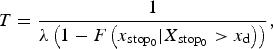 $$T = \displaystyle{1 \over {\lambda \left( {1 - F\left( {{x_{{\rm sto}{{\rm p}_{\rm 0}}}} \vert {X_{{\rm sto}{{\rm p}_{\rm 0}}}} \gt {x_{\rm d}}} \right)} \right)}},$$
where
 $F({x_{{\rm sto}{{\rm p}_{\rm 0}}}})$
is the cumulative distribution function of unperturbed (without dam) runout distances beyond the abscissa x
d.
$F({x_{{\rm sto}{{\rm p}_{\rm 0}}}})$
is the cumulative distribution function of unperturbed (without dam) runout distances beyond the abscissa x
d.
Replacing
 $F({x_{{\rm sto}{{\rm p}_{\rm 0}}}})$
by its expression given by the integral of Eqn (2) leads to the (1 − (1/λT)) quantile (also denoted return level) corresponding to the return period T fully analytically, an enormous practical advantage, i.e.:
$F({x_{{\rm sto}{{\rm p}_{\rm 0}}}})$
by its expression given by the integral of Eqn (2) leads to the (1 − (1/λT)) quantile (also denoted return level) corresponding to the return period T fully analytically, an enormous practical advantage, i.e.:
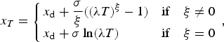 $${x_T} = \left\{ {\matrix{ {{x_{\rm d}} + \displaystyle{\sigma \over \xi} ((\lambda T{)^\xi} - 1)} \hfill & {{\rm if}\quad \xi \ne 0} \hfill \cr {{x_{\rm d}} + \sigma \ln (\lambda T)} \hfill & {{\rm if}\quad \xi = 0} \hfill \cr}} \right.,$$
which is valid for (x T >x d). This expression shows well the crucial role of the sign of the ξ parameter: positive values lead to ‘explosive’ increments of the return level with T, faster than in the exponential case (ξ = 0), for which this increase is log-linear with T. In contrast, in the Weibull case (ξ<0), the quantile, for high values of T, tends to the limit return level x d + |σ/ξ|.
2.1.2. Likelihood maximisation
To get best estimates
 $\hat \lambda $
and
$\hat \lambda $
and
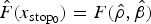 $\hat F({x_{{\rm sto}{{\rm p}_{\rm 0}}}}) = F(\hat \rho, \hat \beta )$
for λ and
$\hat F({x_{{\rm sto}{{\rm p}_{\rm 0}}}}) = F(\hat \rho, \hat \beta )$
for λ and
 $F({x_{{\rm sto}{{\rm p}_{\rm 0}}}})$
, respectively, the standard procedure is to use likelihood maximisation. For the Poisson distribution,
$F({x_{{\rm sto}{{\rm p}_{\rm 0}}}})$
, respectively, the standard procedure is to use likelihood maximisation. For the Poisson distribution,
 $\hat \lambda $
is simply the mean exceedance rate, i.e.
$\hat \lambda $
is simply the mean exceedance rate, i.e.
 $\hat \lambda = m/{T_{{\rm obs}}}$
where
$\hat \lambda = m/{T_{{\rm obs}}}$
where
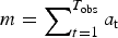 $m = \sum\nolimits_{t = 1}^{{T_{{\rm obs}}}} {{a_{\rm t}}} $
is the number of recorded exceedances of the x
d abscissa during the T
obs winters of observation.
$m = \sum\nolimits_{t = 1}^{{T_{{\rm obs}}}} {{a_{\rm t}}} $
is the number of recorded exceedances of the x
d abscissa during the T
obs winters of observation.
The Generalized Pareto log-likelihood l(ρ, β) is, for β ≠ 0:
 $$\eqalign{l(\rho, \beta ) & = n\log \rho + \left( {\displaystyle{\rho \over \beta} - 1} \right) \cr & \times\sum\limits_{i = 1}^n \log \left( {1 - \beta \left( {{x_{{\rm sto}{{\rm p}_{{0_i}}}}} - {x_{\rm d}}} \right)} \right)},$$
where
 ${x_{{\rm sto}{{\rm p}_{{0_i}}}}}$
, i in [1, n], is an independant and identically distributed sample of the distribution
${x_{{\rm sto}{{\rm p}_{{0_i}}}}}$
, i in [1, n], is an independant and identically distributed sample of the distribution
 $F({x_{{\rm sto}{{\rm p}_{\rm 0}}}})$
.
$F({x_{{\rm sto}{{\rm p}_{\rm 0}}}})$
.
It follows that the maximum log-likelihood estimate for ρ is:
 $$\hat \rho = \displaystyle{n \over {{S_n}\left( {{x_{{\rm sto}{{\rm p}_{\rm 0}}}},\hat \beta} \right)}},$$
where
 $${S_n}\left( {{x_{{\rm sto}{{\rm p}_{\rm 0}}}},\beta} \right) = - \displaystyle{1 \over \beta} \sum\limits_{i = 1}^n \log \left( {1 - \beta \left( {{x_{{\rm sto}{{\rm p}_{{0_i}}}}} - {x_{\rm d}}} \right)} \right).$$
The estimate
 $\hat \beta $
of β is obtained numerically, knowing
$\hat \beta $
of β is obtained numerically, knowing
 $\rho = \hat \rho $
, leading the log-likelihood maximum:
$\rho = \hat \rho $
, leading the log-likelihood maximum:
 $$\hat \beta = \mathop {\max} \limits_\beta l(\hat \rho, \beta ).$$
Classical theory of statistical estimation provides standard errors for the maximum likelihood estimates (MLE) trough:
 $$var(\theta ) = [ - E[H(l \vert \theta {)]]^{ - 1}}$$
where E denotes the mathematical expectation and H(l|θ) is the Hessian matrix of the log-likelihood l indexed by the parameters θ. Specifically, the expression of the negative Hessian of the GPD is (e.g. Coles (Reference Coles2001)):
 $$\hskip-37pt - H(l \vert \theta ) = \left( {\matrix{ {\displaystyle{n \over {{\rho ^2}}}} & {\displaystyle{1 \over \beta} \left( {\sum\nolimits_{i = 1}^n {\displaystyle{{\left( {{x_{{\rm sto}{{\rm p}_{{0_i}}}}} - {x_{\rm d}}} \right)} \over {\left( {1 - \beta \left( {{x_{{\rm sto}{{\rm p}_{{0_i}}}}} - {x_{\rm d}}} \right)} \right)}} - {S_n}\left( {{x_{{\rm sto}{{\rm p}_{\rm 0}}}},\beta} \right)}} \right)} \cr {sym}& \matrix{ - \displaystyle{{2\rho} \over {{\beta ^2}}}\left( {\sum\nolimits_{i = 1}^n {\displaystyle{{\left( {{x_{{\rm sto}{{\rm p}_{{0_i}}}}} - {x_{\rm d}}} \right)} \over {\left( {1 - \beta \left( {{x_{{\rm sto}{{\rm p}_{{0_i}}}}} - {x_{\rm d}}} \right)} \right)}} + {S_n}\left( {{x_{{\rm sto}{{\rm p}_{\rm 0}}}},\beta} \right)}} \right) \hfill \cr + \left( {\displaystyle{\rho \over \beta} - 1} \right)\sum\nolimits_{i = 1}^n {\displaystyle{{{{\left( {{x_{{\rm sto}{{\rm p}_{{0_i}}}}} - {x_{\rm d}}} \right)}^2}} \over {{{\left( {1 - \beta \left( {{x_{{\rm sto}{{\rm p}_{{0_i}}}}} - {x_{\rm d}}} \right)} \right)}^2}}}} \hfill} \cr}} \right),$$
where sym denotes that the matrix is symmetrical. Since MLE are asymptotically Gaussian, these standard errors allow easy construction of asymptotic confidence intervals for the estimated parameters, to fairly represent the uncertainty resulting from the limited data sample available.
2.1.3. Model selection and profile likelihood maximisation
The Poisson – exponential model is a very specific limit case of the Poisson – GPD model (ξ = 0), with a different writing of the likelihood according to Eqn (2). Model selection is typically based on the likelihood ratio test using the D deviance statistics. Specifically, if ℓ1(M
1) is the maximised log-likelihood corresponding to the exponential distribution (β = 0) and ℓ0(M
0) the maximised log-likelihood corresponding to the GPD distribution (β ≠ 0), then D = 2{ℓ1(M
1) − ℓ0(M
0)}. Its asymptotic distribution is given by the one degree of freedom χ
2 law. The null hypothesis is the choice of the exponential model. It is rejected at the
 $\alpha \% $
significance level if
$\alpha \% $
significance level if
 $D \gt {c_{{\alpha _{{\chi ^2}}}}}$
where
$D \gt {c_{{\alpha _{{\chi ^2}}}}}$
where
 ${c_{{\alpha _{{\chi ^2}}}}}$
is the
${c_{{\alpha _{{\chi ^2}}}}}$
is the
 $1 - \alpha \% $
quantile of the one degree of freedom χ
2 (e.g.
$1 - \alpha \% $
quantile of the one degree of freedom χ
2 (e.g.
 ${c_{{\alpha _{{\chi ^2}}}}} = 3.84$
for the 95% quantile).
${c_{{\alpha _{{\chi ^2}}}}} = 3.84$
for the 95% quantile).
The shape parameter ξ (or β) is often difficult to estimate on real data. Besides, the estimates
 $\hat \sigma $
and
$\hat \sigma $
and
 $\hat \xi $
are linked. As a consequence, the likelihood is often very similar around the optimum
$\hat \xi $
are linked. As a consequence, the likelihood is often very similar around the optimum
 $(\hat \sigma, \;\hat \xi )$
, so that different couples (σ, ξ) may well fit the data. To explore the practical implication of that, and hence, to go on with the uncertainty/sensitivity analysis to hazard model choice, we hereafter test different couples obtained by solving the profile likelihood maximisation for various possible values of ξ
0 as:
$(\hat \sigma, \;\hat \xi )$
, so that different couples (σ, ξ) may well fit the data. To explore the practical implication of that, and hence, to go on with the uncertainty/sensitivity analysis to hazard model choice, we hereafter test different couples obtained by solving the profile likelihood maximisation for various possible values of ξ
0 as:
 $$\hat \sigma ({\xi _0}) = \mathop {\arg \min} \limits_\sigma \left( { - \sum\limits_{i = 1}^n \log f\left( {\sigma \vert {x_{{\rm sto}{{\rm p}_i}}},{\xi _0}} \right)} \right).$$
2.2. Avalanche/dam interaction laws
2.2.1. Runout shortening by energy dissipation
It is rarely possible (for economical and/or environmental reasons) to design a catching dam that will stop all avalanches at all times. Some avalanches might overflow the dam and flow downstream. One way of quantifying the residual risk related to overflow is to estimate the avalanche runout shortening caused by the dam,
 ${x_{{\rm stop}}}({h_{\rm d}}) - {x_{{\rm sto}{{\rm p}_{\rm 0}}}}$
where x
xtop(h
d) and
${x_{{\rm stop}}}({h_{\rm d}}) - {x_{{\rm sto}{{\rm p}_{\rm 0}}}}$
where x
xtop(h
d) and
 ${X_{{\rm sto}{{\rm p}_{\rm 0}}}}$
are the maximum runout distances with and without dam, respectively, and h
d is the dam height. A first interaction law was established to relate the maximum runout distance downstream of a dam, x
stop(h
d) relative to the maximum runout distance without the dam,
${X_{{\rm sto}{{\rm p}_{\rm 0}}}}$
are the maximum runout distances with and without dam, respectively, and h
d is the dam height. A first interaction law was established to relate the maximum runout distance downstream of a dam, x
stop(h
d) relative to the maximum runout distance without the dam,
 ${X_{{\rm sto}{{\rm p}_{\rm 0}}}}$
, to the dam height h
d relative to the thickness of the incident avalanche-flow h
0 as:
${X_{{\rm sto}{{\rm p}_{\rm 0}}}}$
, to the dam height h
d relative to the thickness of the incident avalanche-flow h
0 as:
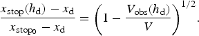
 $$\displaystyle{{{x_{{\rm stop}}}({h_{\rm d}}) - {x_{\rm d}}} \over {{x_{{\rm sto}{{\rm p}_{\rm 0}}}} - {x_{\rm d}}}} = 1 - \alpha \displaystyle{{{h_{\rm d}}} \over {{h_0}}}.$$
Here, α is the energy dissipation coefficient quantifying the dam efficiency. It is assumed to be constant and equal to 0.14 in the present study. Due to Eqns (2) and (9), x stop(h d) is also GPD-distributed when considering the runout shortening by energy dissipation.
This interaction law was initially developed by Faug and others (Reference Faug, Naaim, Bertrand, Lachamp and Naaim-Bouvet2003), further justified and verified by Faug and others (Reference Faug, Gauer, Lied and Naaim2008), and previously used for risk and optimal design computations by Eckert and others (Reference Eckert, Parent, Faug and Naaim2008, Reference Eckert, Parent, Faug and Naaim2009, Reference Eckert2012). It is expected to be valid when local dissipations of kinetic energy prevail, which are generally verified under two conditions: (1) fast dry snow avalanches (inertial regime) characterised by relatively high Froude numbers (5–10) and (2) a dam height not too high, in order to prevent the formation of shocks upstream of the dam. If the dam height is too high, typically h d/h 0 5–11 for Froude numbers in the range 5–10, propagating waves are likely to be formed upstream of the dam, which may lead to large volumes of snow retained upstream.
A positivity constraint exists with this interaction law, i.e. h d <(h 0/α). For higher dams, all avalanches are stopped. For instance, for an incident avalanche flow h 0 = 1 m, h d is in the [0 m, 7.14 m] interval. Another critical upper value for the dam height that avoids the formation of shocks upstream of the dam can also be determined according to the Froude number of the flow. In theory, this critical value can be lower or >h 0/α. In this paper, however, we avoid this difficulty by investigating only Froude number ranges for which the minimal height for shock formation is >h 0/α.
2.2.2. Runout shortening by volume catch
Another interaction law relates the maximum runout distance downstream of the dam, x
stop(h
d) relative to the runout distance without the dam,
 ${X_{{\rm sto}{{\rm p}_{\rm 0}}}}$
, to the dam height. However, it is somewhat different because it is based on the idea that the runout shortening is mainly driven by the volume reduction. As a natural deposit, caused by friction with the bottom, is likely to occur with or without the presence of the obstacle (Faug and others, Reference Faug, Naaim and Naaim-Bouvet2004), the volume retained upstream of the dam is the sum of this natural volume due to friction, V
stop and the volume retained by the obstacle only, V
obs(h
d), which depends on the dam height (Fig. 1). Specifically, under the assumption of a very slow avalanche (Froude number < 1), Faug (Reference Faug2004) proposed:
${X_{{\rm sto}{{\rm p}_{\rm 0}}}}$
, to the dam height. However, it is somewhat different because it is based on the idea that the runout shortening is mainly driven by the volume reduction. As a natural deposit, caused by friction with the bottom, is likely to occur with or without the presence of the obstacle (Faug and others, Reference Faug, Naaim and Naaim-Bouvet2004), the volume retained upstream of the dam is the sum of this natural volume due to friction, V
stop and the volume retained by the obstacle only, V
obs(h
d), which depends on the dam height (Fig. 1). Specifically, under the assumption of a very slow avalanche (Froude number < 1), Faug (Reference Faug2004) proposed:
 $$\displaystyle{{{x_{{\rm stop}}}({h_{\rm d}}) - {x_{\rm d}}} \over {{x_{{\rm sto}{{\rm p}_{\rm 0}}}} - {x_{\rm d}}}} = {\left( {1 - \displaystyle{{{V_{{\rm obs}}}({h_{\rm d}})} \over {V - {V_{{\rm stop}}}}}} \right)^n},$$
where V is the avalanche flow volume and n can be either 1/2 or 1/3, depending on the characteristics of the upstream storage zone (confined or not). For a confined storage zone, n = 1/2 is more suitable. Furthermore, the reasonable assumption that V stop is much smaller that V obs yields:
 $$\displaystyle{{{x_{{\rm stop}}}({h_{\rm d}}) - {x_{\rm d}}} \over {{x_{{\rm sto}{{\rm p}_{\rm 0}}}} - {x_{\rm d}}}} = {\left( {1 - \displaystyle{{{V_{{\rm obs}}}({h_{\rm d}})} \over V}} \right)^{1/2}}.$$

Fig. 1. Definition of deposited volumes without (a) and with (b) obstacle (dam of height h d at the abscissa x d), inspired by Faug (Reference Faug2004).
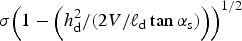
Due to Eqns (2) and (11), x stop(h d) is also GPD-distributed when considering the runout shortening by volume catch. Finally, by assuming that the volume V obs(h d) stored upstream of the dam roughly has a triangular shape forming a line inclined at constant slope ϕ with the horizontal, one can explicitly relate the retained volume to the dam height h d when the deposit zone upstream of the dam is confined and of constant width ℓd. However, the shape of the deposit V obs might depend on the snow type, i.e. dry snow versus more humid snow, so that one may expect two situations to occur, described by:
 $${V_{{\rm obs}}}({h_{\rm d}}) = \displaystyle{{{\ell _{\rm d}} \times h_{\rm d}^{\rm 2}} \over {2\;{\rm tan}({\alpha _{\rm s}})}},$$
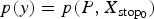
with α s = ψ fz − ϕ, where the length L of the deposit upstream the dam is L = h d/tan (α s), ϕ is the angle of snow deposit (i.e. the angle with the horizontal measured in the inverse trigonometric wise, that could be <0, e.g. Fig. 2a or ≥0, e.g. Fig. 2b) and ψ fz is the angle of the slope.

Fig. 2. Difference in deposit shape assumed in this study between ‘dry’ and ‘humid’ snow avalanches, ϕ = 0° is the limit case between these. Other given ϕ values are those considered in text.
For humid snow (very slow flows), the friction coefficient, classically denoted as μ in the avalanche literature, should be high (e.g. Naaim and others, Reference Naaim, Durand, Eckert and Chambon2013), resulting in larger deposits with a deposit line above the horizontal plane. In contrast, dry cold snow should flow faster with a lower friction coefficient, resulting in longer deposits with a deposit line below the horizontal plane. All assumptions and notations regarding runout shortening by volume catch are outlined in Figure 2.
In practice, the volume stored upstream of the dam is smaller or equal to the incident avalanche volume leading to the constraint h
d < (V × 2 tan (α
s)/ℓd)1/2. The positivity constraint associated with Eqn (11) then becomes:
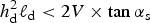 $h_{\rm d}^{\rm 2} {\ell _{\rm d}} \lt 2V \times \tan {\alpha _{\rm s}}$
, which is equivalent to h
d < (2V/ℓdtan
α
s)1/2. For example, for an incident volume V = 50 000 m3, ϕ = 0°, ψ
fz = 10° and ℓd = 100 m, h
d is in the [0, 18.7] interval.
$h_{\rm d}^{\rm 2} {\ell _{\rm d}} \lt 2V \times \tan {\alpha _{\rm s}}$
, which is equivalent to h
d < (2V/ℓdtan
α
s)1/2. For example, for an incident volume V = 50 000 m3, ϕ = 0°, ψ
fz = 10° and ℓd = 100 m, h
d is in the [0, 18.7] interval.
All in all, these considerations highlight that the runout shortening according to volume catch relation is much more flexible than that regarding energy dissipation. Indeed, whereas in Eqns (9–12) an avalanche scenario is a flow depth and a volume, respectively, with the volume catch relation, one has, in addition, the deposit angle ϕ (value and sign) to specify, according to the snow type one considers.
2.3. Individual risk and optimal design based on its minimisation
2.3.1. Specific risk
Among natural hazards, risk is broadly defined as an expected damage, in accordance with mathematical theory (e.g. Merz and others (Reference Merz, Kreibich, Schwarze and Thieken2010) for floods, Mavrouli (Reference Mavrouli2010) for rockfalls, Jordaan (Reference Jordaan2005) in engineering, etc.). Following the notation of Eckert and others (Reference Eckert2012), the specific risk r z for an element at risk z is:
 $${r_{\rm z}} = \lambda \int p(y){{\cal V}_{\rm z}}(y)\;{\rm d}y,$$
where λ is the annual avalanche rate, i.e. the annual frequency occurrence of an avalanche, p(y) is the multivariate avalanche intensity distribution (runout, flow depth, etc.) and
 ${{\cal V}_{\rm z}}(y)$
is the vulnerability of the element z to the avalanche intensity y.
${{\cal V}_{\rm z}}(y)$
is the vulnerability of the element z to the avalanche intensity y.
 ${{\cal V}_{\rm z}}(y)$
can be either a damage level or a destruction rate, depending if a deterministic or a probabilistic (relability based) point of view is adopted. By definition, the specific risk unit at the annual timescale is a–1.
${{\cal V}_{\rm z}}(y)$
can be either a damage level or a destruction rate, depending if a deterministic or a probabilistic (relability based) point of view is adopted. By definition, the specific risk unit at the annual timescale is a–1.
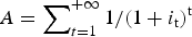
In accordance with our hazard and interaction law model specifications, we describe avalanche flow within a two-dimensional cartesian frame. In it, avalanche intensity y is classically defined by the joint distribution of the pressure P and the runout distance
 ${X_{{\rm sto}{{\rm p}_{\rm 0}}}}$
such as
${X_{{\rm sto}{{\rm p}_{\rm 0}}}}$
such as
 $p(y) = p(P,{X_{{\rm sto}{{\rm p}_{\rm 0}}}})$
of pressure fields P and runout distances
$p(y) = p(P,{X_{{\rm sto}{{\rm p}_{\rm 0}}}})$
of pressure fields P and runout distances
 ${X_{{\rm sto}{{\rm p}_{\rm 0}}}}$
. The specific risk r
b(x
b) for the element b at the x
b abscissa is then:
${X_{{\rm sto}{{\rm p}_{\rm 0}}}}$
. The specific risk r
b(x
b) for the element b at the x
b abscissa is then:
 $$\eqalign{r_{\rm b}(x_{\rm b}) & = \lambda \int p\left( {P \vert \, {x_{\rm b}} \le {X_{{\rm sto}{{\rm p}_{\rm 0}}}}} \right)p\left( {{x_{\rm b}} \le {X_{{\rm sto}{{\rm p}_0}}}} \right) \cr & \times {{\cal V}_{\rm b}}(P)\;{\rm d}P,} $$
where the notation ‘.|.’ classically denotes a conditional probability. Notations x
b,
 ${{\cal V}_{\rm b}}$
and r
b (indice b) indicate that the typical element at risk we consider is a building.
${{\cal V}_{\rm b}}$
and r
b (indice b) indicate that the typical element at risk we consider is a building.
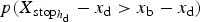
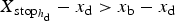
We consider only building abscissas such as x b > x d, a natural choice in practice (one would not build further up in the path for evident safety reasons), which makes the link with our POT approach. Hence, the λ avalanche rate in Eqn (14) can be assimilated to the occurrence rate in Eqn (1). Also, the over threshold x b > x d condition should appear in all risk equations (Eqn (14) and the following), but it is dropped, for simplicity.
2.3.2. Residual risk and optimal design
The dam optimal design approach we consider minimises the long-term costs obtained by summing the construction costs and the expected damages for the building at abscissa x b. The underlying mathematical theory (Von Neumann and Morgenstern, Reference Von Neumann and Morgenstern1953; Raiffa, Reference Raiffa1968) has been adapted to avalanche engineering by Eckert and others (Reference Eckert, Parent, Faug and Naaim2008, Reference Eckert, Parent, Faug and Naaim2009), in analogy to the precursory work by Van Danzig (Reference Van Danzig1956) for maritime dykes in Holland and by Bernier (Reference Bernier2003) for river dams. Hence, the long-term costs with a protective dam h d are:
 $$\eqalign{R({x_{\rm b}},{h_{\rm d}}) = & {\;C_0}{h_{\rm d}} + {C_1}A\lambda \!{\int}\! p\left( {{P_{{h_{\rm d}}}},\;{x_{\rm b}} \le {X_{{\rm sto}{{\rm p}_{{h_{\rm d}}}}}}} \right) \cr & \times p\left( {{x_{\rm b}} \le {X_{{\rm sto}{{\rm p}_{{h_{\rm d}}}}}}} \right) \times {{\cal V}_{\rm z}}(P)\;{\rm d}P,} $$
where C
1 and C
0 are, respectively, the value of the building at risk at abscissa x
b in €, the monetary currency we work with, and the value of the dam per meter height, €.m
−1. The actualisation factor to pass from annual to long-term risk is
 $A = \sum\nolimits_{t = 1}^{ + \infty} {1/{{(1 + {i_{\rm t}})}^{\rm t}}} $
with i
t the interest rate for the year t. The unit of the long-term costs R(x
b, h
d) is therefore €. The subscript notation ‘
$A = \sum\nolimits_{t = 1}^{ + \infty} {1/{{(1 + {i_{\rm t}})}^{\rm t}}} $
with i
t the interest rate for the year t. The unit of the long-term costs R(x
b, h
d) is therefore €. The subscript notation ‘
 $_{{h_{\rm d}}} $
’ in Eqn (15) denotes that runout and pressure distributions are now modified in the runout zone, conditional to the dam height h
d. As a consequence, for a fixed h
d value, the long-term costs correspond to the residual risk after the dam construction.
$_{{h_{\rm d}}} $
’ in Eqn (15) denotes that runout and pressure distributions are now modified in the runout zone, conditional to the dam height h
d. As a consequence, for a fixed h
d value, the long-term costs correspond to the residual risk after the dam construction.
We stress that R(x b, h d) is nothing more than C 0 h d + C 1 Ar b(x b, h d), with r b(x b, h d) the specific residual risk at the annual timescale for the building at the abscissa x b, defined as Eqn (14) but with the dam height h d. This highlights that the approach remains individual risk based, with one single element at risk at abscissa position x b. Note also that the damages caused to the dam by successive avalanches and the consecutive reparation costs do not appear explicitly in Eqn (15). In fact, they are included in the C 0 evaluation through the definition of a suitable amortising period, a straightforward econometrical computation. Yet, a strong underlying assumption is made: in case an avalanche severely damages or even destroys the dam, the dam still reduces the hazard for this specific avalanche event according to Eqns (9) or (11), and is repaired immediately thereafter.
Strong simplifications occur if the additional assumption of a constant step vulnerability function is made. The worst-case scenario is that the damage is maximal as soon as the element at risk is attained, whereas the considered element at risk remains obviously undamaged if the avalanche does not reach its abscissa. The integral in Eqn (15) is then reduced to
 $p({X_{{\rm sto}{{\rm p}_{{h_{\rm d}}}}}} - {x_{\rm d}} \gt {x_{\rm b}} - {x_{\rm d}})$
, the probability of exceeding the abscissa x
b with a protective dam height h
d, so that:
$p({X_{{\rm sto}{{\rm p}_{{h_{\rm d}}}}}} - {x_{\rm d}} \gt {x_{\rm b}} - {x_{\rm d}})$
, the probability of exceeding the abscissa x
b with a protective dam height h
d, so that:
 $$R({x_{\rm b}},{h_{\rm d}}) = {C_0}{h_{\rm d}} + \lambda {C_1}A\left( {1 - {F_{{h_{\rm d}}}}({x_{\rm b}} - {x_{\rm d}})} \right),$$
where
 ${F_{{h_{\rm d}}}}({x_{\rm b}} - {x_{\rm d}})$
is the cumulative distribution function of runouts in x
b with a protective dam height h
d. This is the key assumption to keep a fully analytical decisional model with our POT approach.
${F_{{h_{\rm d}}}}({x_{\rm b}} - {x_{\rm d}})$
is the cumulative distribution function of runouts in x
b with a protective dam height h
d. This is the key assumption to keep a fully analytical decisional model with our POT approach.
Equation (16) can first be regarded as a residual risk function that, for a fixed value of h
d, varies according to the x
b position. It is then a linear function of the non-exceedance probability
 ${F_{{h_{\rm d}}}}({x_{\rm b}} - {x_{\rm d}})$
showing the decrease of the residual risk in the runout zone as one goes further and further away downstream. This directly represents/illustrates the coupling of the interaction law with the probabilistic POT hazard model. Second, Eqn (16) can be regarded as total costs depending on the dam height h
d at a fixed x
b position, for instance a specific position of the runout zone, which has some legal meaning (such as the limit of a hazard zone), or a position where a real element at risk/building is situated. The optimal dam height from a stake holder's perspective is then simply:
${F_{{h_{\rm d}}}}({x_{\rm b}} - {x_{\rm d}})$
showing the decrease of the residual risk in the runout zone as one goes further and further away downstream. This directly represents/illustrates the coupling of the interaction law with the probabilistic POT hazard model. Second, Eqn (16) can be regarded as total costs depending on the dam height h
d at a fixed x
b position, for instance a specific position of the runout zone, which has some legal meaning (such as the limit of a hazard zone), or a position where a real element at risk/building is situated. The optimal dam height from a stake holder's perspective is then simply:
 $$h_{\rm d}^{\rm {\ast}} = \mathop {\arg \min} \limits_{{h_{\rm d}}} (R({x_{\rm b}},{h_{\rm d}})),$$
where the function
 $\arg \min $
gives, for a given x
b, the height h
d at which R is minimal.
$\arg \min $
gives, for a given x
b, the height h
d at which R is minimal.
2.3.3. Explicit risk formulae with the energy dissipation interaction law
According to Eqn (9), under the constraint h d <(h 0/α), one has
 $$P\left( {{X_{{\rm sto}{{\rm p}_{{h_{\rm d}}}}}} - {x_{\rm d}} \gt {x_{\rm b}} - {x_{\rm d}}} \right) = P\left( {{\textstyle{{{X_{{\rm sto}{{\rm p}_0}}} - {x_{\rm d}}} \over {1 - \alpha ({h_{\rm d}}/{h_0})}}} \gt {x_{\rm b}} - {x_{\rm d}}} \right).$$
In other words, the random variable
 ${X_{{\rm sto}{{\rm p}_{{h_{\rm d}}}}}} - {x_{\rm d}}$
remains GPD distributed, with the same shape parameter ξ as
${X_{{\rm sto}{{\rm p}_{{h_{\rm d}}}}}} - {x_{\rm d}}$
remains GPD distributed, with the same shape parameter ξ as
 ${X_{{\rm sto}{{\rm p}_{\rm 0}}}} - {x_{\rm d}}$
, but with the modified scale parameter σ(1 − α(h
d/h
0)). The expression of the residual risk for the Poisson – GPD decisional model is straightforward:
${X_{{\rm sto}{{\rm p}_{\rm 0}}}} - {x_{\rm d}}$
, but with the modified scale parameter σ(1 − α(h
d/h
0)). The expression of the residual risk for the Poisson – GPD decisional model is straightforward:
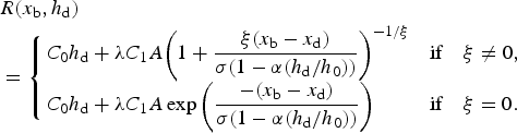 $$\eqalign{& R(x_{\rm b},{h_{\rm d}}) \cr & = \left\{ {\matrix{ {{C_0}{h_{\rm d}} + \lambda {C_1}A{{\left( {1 + \displaystyle{{\xi ({x_{\rm b}} - {x_{\rm d}})} \over {\sigma (1 - \alpha ({h_{\rm d}}/{h_0}))}}} \right)}^{ - 1/\xi}}} \hfill & {{\rm if}\quad \xi \ne 0,} \hfill\cr {{C_0}{h_{\rm d}} + \lambda {C_1}A\exp \left( {\displaystyle{{ - ({x_{\rm b}} - {x_{\rm d}})} \over {\sigma (1 - \alpha ({h_{\rm d}}/{h_0}))}}} \right)} \hfill & {{\rm if}\quad \xi = 0.} \hfill \cr}} \right.}$$
2.3.4. Explicit risk formulae with the volume catch interaction law
According to Eqn (11), under the constraint h d <(2V/ℓd tan α s)1/2, one has this time
 $$P\left( {{X_{{\rm sto}{{\rm p}_{{h_{\rm d}}}}}} - {x_{\rm d}} \gt {x_{\rm b}} - {x_{\rm d}}} \right) = P\left( {{\textstyle{{{X_{{\rm sto}{{\rm p}_0}}} - {x_{\rm d}}} \over {{{\left( {1 - \left( {{{h_{\rm d}^{\rm 2}} / {(2V/{\ell _{\rm d}}\tan {\alpha _{\rm s}}}})} \right)} \right)}^{1/2}}}}} \gt {x_{\rm b}} - {x_{\rm d}}} \right).$$
Hence,
 ${X_{{\rm sto}{{\rm p}_{{h_{\rm d}}}}}} - {x_{\rm d}}$
is once again still GPD-distributed, but this time with the modified scale parameter
${X_{{\rm sto}{{\rm p}_{{h_{\rm d}}}}}} - {x_{\rm d}}$
is once again still GPD-distributed, but this time with the modified scale parameter
 $\sigma {\left( {1 - \left( {{{h_{\rm d}^{\rm 2}} / {(2V/{\ell _{\rm d}}\tan {\alpha _{\rm s}}}})} \right)} \right)^{1/2}}$
, leading the residual risk:
$\sigma {\left( {1 - \left( {{{h_{\rm d}^{\rm 2}} / {(2V/{\ell _{\rm d}}\tan {\alpha _{\rm s}}}})} \right)} \right)^{1/2}}$
, leading the residual risk:
 $$ R({x_{\rm b}},{h_{\rm d}}) = \left\{ {\matrix{ {{C_0}{h_{\rm d}} + \lambda {C_1}A{{\left( {1 + \displaystyle{{\xi ({x_{\rm b}} - {x_{\rm d}})} \over {\sigma {{\left( {1 - \left( {{{h_{\rm d}^{\rm 2}} / {(2V/{\ell _{\rm d}}\tan {\alpha _{\rm s}}}})} \right)} \right)}^{1/2}}}}} \right)}^{ - 1/\xi}}} \hfill & {{\rm if}\quad \xi \ne 0,} \hfill \cr {{C_0}{h_{\rm d}} + A\lambda {C_1}\left( {\exp \left( {\displaystyle{{ - ({x_{\rm b}} - {x_{\rm d}})} \over {\sigma {{\left( {1 - \left( {{{h_{\rm d}^{\rm 2}} / {(2V/{\ell _{\rm d}}\tan {\alpha _{\rm s}}}})} \right)} \right)}^{1/2}}}}} \right)} \right)} \hfill & {{\rm if}\quad \xi = 0,} \hfill \cr}} \right.$$
where tan(α s) = tan(ψ fz − ϕ) and ϕ is arbitrary negative for dry snow avalanches and positive for humid snow avalanches, with the standard limit case ϕ = 0 (Fig. 2).
2.3.5. Solutions to the risk minimisation problem
None of these risk equations provide analytical solutions to Eqn (17). As a consequence, this is where a numerical search is required, spanning, for a fixed x b position, the possible values of h d. With the energy dissipation law, this has already been demonstrated by Eckert and others (Reference Eckert, Parent, Faug and Naaim2008) for the Poisson – exponential case. For the volume catch interaction law, however, because of the higher complexity of the dependency of R(x b, h d) on h d, different typical cases can be encountered: no optimum, one ‘pseudo’ optimum due to the positivity constraint, and the ‘good’ case of a minimum residual risk arising as an optimal compromise between losses and construction costs. Yet, in the latter case, relative maximum residual risks can also be observed. These different cases are detailed in Appendix. For our application, we identified which of them occurred in all configurations we tested, and only dam heights truly minimising the risk were kept. These correspond to optimal compromises between construction costs and losses, but also to the pseudo optima, i.e. dam heights just sufficient to stop all avalanches before the considered building position.
2.4. Quantifying uncertainty and sensitivity: intervals, bounds and indexes
Since one objective of this paper is to quantify how risk estimates and optimal design values vary across runout tail distribution types and avalanche/dam interaction laws, we propose different intervals, bounds and indexes suitable for taking into account different types of uncertainty/variability. These intervals, bounds and indexes may be usable by engineers in risk zoning and defense structure design to represent sensitivity to available data resulting from parameter estimate standard errors, and/or sensitivity to non-probabilistic model uncertainty. They also have wider interest, being somewhat interpretable in terms of respective weight of the different ingredients of the decisional analysis.
With regard to the difference to be made between model parameters and their estimates on the basis of the available data, all risk computations are performed under the classical paradigm of statistical inference. This means that we plug the maximum full/profile likelihood estimates
 $(\hat \lambda, \;\hat \xi, \;\hat \sigma )$
or
$(\hat \lambda, \;\hat \xi, \;\hat \sigma )$
or
 $(\hat \lambda, \;\hat \sigma ({\xi _0}))$
into the Poisson – GPD model, and we evaluate return levels and risk functions accordingly, considering
$(\hat \lambda, \;\hat \sigma ({\xi _0}))$
into the Poisson – GPD model, and we evaluate return levels and risk functions accordingly, considering
 $R({x_{\rm b}},\;{h_{\rm d}},\;\hat \lambda, \;\hat \xi, \;\hat \sigma )$
or
$R({x_{\rm b}},\;{h_{\rm d}},\;\hat \lambda, \;\hat \xi, \;\hat \sigma )$
or
 $R({x_{\rm b}},\;{h_{\rm d}},\;\hat \lambda, \;\hat \sigma ({\xi _0}))$
. Here, and in all that follows, the notation ξ
0 indicates that the GPD shape parameter is chosen and that the profile likelihood is maximised conditionally to its choice.
$R({x_{\rm b}},\;{h_{\rm d}},\;\hat \lambda, \;\hat \sigma ({\xi _0}))$
. Here, and in all that follows, the notation ξ
0 indicates that the GPD shape parameter is chosen and that the profile likelihood is maximised conditionally to its choice.
2.4.1. Propagating uncertainty on parameter estimates
To quantify the uncertainty resulting from the limited data sample available, the usual approach is to propagate parameter standard errors (Eqn (6)) up to the quantities of interest. Starting from the MLE for the Poisson – GPD model and the associated asymptotic variance-covariance matrix, different methods exist in the literature to evaluate confidence intervals for high-return levels. Appendix presents how the, arguably, two most common of them can be adapted to the profile likelihood case, where the shape parameter value ξ 0 results from a more or less arbitrary modelling choice rather than from inference.
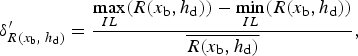
2.4.2. Bounds and sensitivity indexes to the runout tail shape
From a different perspective, to evaluate the influence of the runout tail shape, we evaluate Eqns (18) and (19) according to the range of ξ
0 values provided by the profile likelihood maximisation procedure, i.e. when ξ
0 takes diferent values in the range [−0.3, 1.3]. We do that without a dam, and also for a given dam height and interaction law. From this set of values (one for each ξ
0), retaining the maximum and minimum risk value at each abscissa leads to risk bound functions of the abscissa, interaction law and dam height. They constitute plausible upper/lower bounds for the risk, taking into account the variability of risk estimates towards runout distribution tail types. To summarise the spread at the abscissa x
b, the sensitivity index
 ${\delta _{R({x_{_{\rm b}}}, \;{h_{_{\rm d}}} )}}$
is evaluated:
${\delta _{R({x_{_{\rm b}}}, \;{h_{_{\rm d}}} )}}$
is evaluated:
 $${\delta _{R({x_{_{\rm b}}}, \;{h_{_{\rm d}}} )}} = \displaystyle{{\mathop {\max} \limits_{{\xi _0}} (R({x_{\rm b}},{h_{\rm d}})) - \mathop {\min} \limits_{{\xi _0}} (R({x_{\rm b}},{h_{\rm d}}))} \over {\overline {R({x_{\rm b}},{h_{\rm d}})}}}$$
with
 $\overline {R({x_{\rm b}},\;{h_{\rm d}})} $
, the mean value evaluated at the abscissa x
b with the dam height h
d. With the different interaction laws at hand (energy dissipation and volume catch with varying deposit shape angles), different values of
$\overline {R({x_{\rm b}},\;{h_{\rm d}})} $
, the mean value evaluated at the abscissa x
b with the dam height h
d. With the different interaction laws at hand (energy dissipation and volume catch with varying deposit shape angles), different values of
 ${\delta _{R({x_{_{\rm b}}}, \;{h_{_{\rm d}}} )}}$
can be obtained.
${\delta _{R({x_{_{\rm b}}}, \;{h_{_{\rm d}}} )}}$
can be obtained.
To do a similar evaluation for the optimal design procedure, we also search for a given position x
b and interaction law, the solution
 $h_{\rm d}^{\ast} $
of Eqn (17) for each possible value ξ
0. The solution spread towards runout tail shapes is quantified from the minimum, maximum and mean optimal height at the abscissa x
b, denoted
$h_{\rm d}^{\ast} $
of Eqn (17) for each possible value ξ
0. The solution spread towards runout tail shapes is quantified from the minimum, maximum and mean optimal height at the abscissa x
b, denoted
 $h_{\rm d}^{\ast} ({x_{\rm b}})$
as:
$h_{\rm d}^{\ast} ({x_{\rm b}})$
as:
 $${\delta _{{x_{\rm b}},h_{\rm d}^{\rm {^\ast}}}} = \displaystyle{{\mathop {\max} \limits_{{\xi _0}} \left( {h_{\rm d}^{\rm {^\ast}} ({x_{\rm b}})} \right) - \mathop {\min} \limits_{{\xi _0}} \left( {h_{\rm d}^{\rm {^\ast}} ({x_{\rm b}})} \right)} \over {\overline {h_{\rm d}^{\rm {^\ast}} ({x_{\rm b}})}}}. $$
Finally, to confront risk and optimal design sensitivity to the ξ 0 choice, we evaluate the same sensitivity index function and interaction law as:
 $${\delta _{R({x_{\rm b}},\;h_{\rm d}^{\rm {^\ast}} )}} = \displaystyle{{\mathop {\max} \limits_{{\xi _0}} \left( {R(h_{\rm d}^{\rm {^\ast}} ({x_{\rm b}}))} \right) - \mathop {\min} \limits_{{\xi _0}} \left( {R(h_{\rm d}^{\rm {^\ast}} ({x_{\rm b}}))} \right)} \over {\overline {R(h_{\rm d}^{\rm {^\ast}} ({x_{\rm b}}))}}}, $$
where
 $R(h_{\rm d}^{\ast} ({x_{\rm b}}))$
denotes the minimum residual risk at the abscissa x
b given
$R(h_{\rm d}^{\ast} ({x_{\rm b}}))$
denotes the minimum residual risk at the abscissa x
b given
 ${h_{\rm d}} = h_{\rm d}^{\ast} ({x_{\rm b}})$
. Note that the latter index is somewhat different from that provided by Eqn (20) where h
d was fixed once for all. This time, for each value ξ
0, the dam height considered to evaluate the risk is different, as it is the one that locally minimises the residual risk.
${h_{\rm d}} = h_{\rm d}^{\ast} ({x_{\rm b}})$
. Note that the latter index is somewhat different from that provided by Eqn (20) where h
d was fixed once for all. This time, for each value ξ
0, the dam height considered to evaluate the risk is different, as it is the one that locally minimises the residual risk.
2.4.3. Bounds and sensitivity index to the avalanche/dam interaction law
Similarly, to evaluate the sensitivity to the choice of one interaction law instead of another, we evaluate, for a given runout tail (ξ 0 is fixed), abscissa x b and dam height h d, the spread between the possible risk estimates as:
 $${\delta ^{\prime}_{R({x_{\rm b}},\;{h_{\rm d}})}} = \displaystyle{{\mathop {\max} \limits_{IL} (R({x_{\rm b}},{h_{\rm d}})) - \mathop {\min} \limits_{IL} (R({x_{\rm b}},{h_{\rm d}}))} \over {\overline {R({x_{\rm b}},{h_{\rm d}})}}}, $$
where IL is the interaction law considered: the volume catch interaction law with various deposit angles plus potentially, the energy dissipation interaction law.
3. APPLICATION AND RESULTS
3.1. Case study
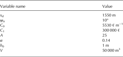
The case study selected is situated in the township of Bessans, French Alps. The runout zone is a gentle slope, making the use of a simple stochastic model for runout distances such as the POT-GPD possible. It is, up to now, free from permanent habitations, but, due to demographic pressure, may become urbanized in the future, provided risk is estimated to be low enough in the current state or after a permanent defense structure construction. Hence, we study the potential risk reduction by a dam at the abscissa x d, which corresponds to the beginning of the runout zone according to a classical slope criterion. During the 1973–2003 period, 28 avalanches exceeding x d were recorded by the local forestry service. The risk evaluation and sensitivity analysis is performed throughout the runout zone. However, for being less case-study dependant in our conclusions, specific positions of legal importance are studied, corresponding to return periods of 10 a–ka. Table 1 summarises the constants fixed through the whole work.
Table 1. Constants used for the case study
3.2. Fitted runout distance/return period relationships
3.2.1. Without dam
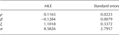
The maximum likelihood method supplies estimates for the Poisson (
 $\hat \lambda = 0.904$
) and the GPD parameters (Table 2). The likelihood ratio test rejects the exponential distribution to the benefit of the GPD distribution at the 5% significance level. The positivity of
$\hat \lambda = 0.904$
) and the GPD parameters (Table 2). The likelihood ratio test rejects the exponential distribution to the benefit of the GPD distribution at the 5% significance level. The positivity of
 $\hat \xi $
, indicates that the best fitted GPD distribution belongs to the Fréchet domain and has therefore a heavy tail. However, the maximum likelihood estimate
$\hat \xi $
, indicates that the best fitted GPD distribution belongs to the Fréchet domain and has therefore a heavy tail. However, the maximum likelihood estimate
 ${\hat \xi _{MLE}}$
is close to 1.1, suggesting a tail so heavy that it should be viewed with distrust since ξ values >0.5 are known to be rare in environmental systems. Furthermore, the associated standard error is very high (Table 2). As a consequence, the high-return levels predicted on the basis of the MLE are presumably unrealistic and, anyhow, the associated confidence intervals provided by the two uncertainty propagation methods we have implemented are so large that they are practically useless (Tables 4, 5). These results highlight that it is not possible to fit a reliable runout tail for this case study on the basis of the data only.
${\hat \xi _{MLE}}$
is close to 1.1, suggesting a tail so heavy that it should be viewed with distrust since ξ values >0.5 are known to be rare in environmental systems. Furthermore, the associated standard error is very high (Table 2). As a consequence, the high-return levels predicted on the basis of the MLE are presumably unrealistic and, anyhow, the associated confidence intervals provided by the two uncertainty propagation methods we have implemented are so large that they are practically useless (Tables 4, 5). These results highlight that it is not possible to fit a reliable runout tail for this case study on the basis of the data only.
Table 2. MLE and respective standard errors for the GPD parameters with the two possible parametrisations
Our profile likelihood approach introduces extra-data information into the analysis through the choice of a ξ 0 value, somewhat arbitrary, but at least in a realistic range. Figure 3a confirms that the likelihood of the data sample under the GPD model is flat around the MLE couple, so that a wide range of other couples may nearly be as suitable in terms of data fitting (Table 3). This is even clearer when the different fitted models are compared with the data (Fig. 3b). We note that the minimum negative log-likelihood increases with decreasing values of ξ 0, suggesting a little more confidence in a heavy tail (positive shape parameter) than in other runout types (null or negative shape parameter; Table 3).

Fig. 3. Model fit and checking: negative log-likelihood curves, density plots and return level plots. Exp is the exponential case (ξ 0 = 0). (a) Profile negative log-likelihoods: green squares denote the minimum of each curve. (b) Density functions provided by the profile likelihood minimisation method versus histogram of original data. (c) Return level plots provided by the profile likelihood minimisation method with original data in red circles.
Table 3. Full and profile likelihood estimates (nll is the minimum negative log-likelihood in each case and * stands for the exponential case where ξ 0 = 0)

The ξ
0 choice, however, considerably impacts the estimated runout distance/return period relationship, for instance the high-return levels of interest for hazard mapping (Fig. 3c). The values of ξ
0 < 0.5 provide
 ${\hat x_{100}}$
−
${\hat x_{100}}$
−
 ${\hat x_{1000}}$
arguably plausible return levels from the perspective of an expert analysis of the path. In contrast, these are clearly too high for ξ
0 > 0.5, as expected with regard to the poor confidence we may have in ξ
0 values >0.5. As a consequence, in the following, we concentrate our analysis on ξ
0 = {−0.3; − 0.1; 0; 0.1; 0.3; 0.5}, i.e. on a range of plausible values containing the three different runout tail types, but with more weight on the heavy tail Fréchet type, according to the information the data seems to contain. Furthermore, in the same spirit, when a single value is required, we focus on ξ
0 = 0.3.
${\hat x_{1000}}$
arguably plausible return levels from the perspective of an expert analysis of the path. In contrast, these are clearly too high for ξ
0 > 0.5, as expected with regard to the poor confidence we may have in ξ
0 values >0.5. As a consequence, in the following, we concentrate our analysis on ξ
0 = {−0.3; − 0.1; 0; 0.1; 0.3; 0.5}, i.e. on a range of plausible values containing the three different runout tail types, but with more weight on the heavy tail Fréchet type, according to the information the data seems to contain. Furthermore, in the same spirit, when a single value is required, we focus on ξ
0 = 0.3.
In more detail, one may note that the concave/convex shape of return level plots with positive/negative ξ 0 values, respectively, makes return levels higher in the Weibull domain (ξ 0 < 0) for ‘low’ return periods, but much higher in the Fréchet domain (ξ 0 >0) for high-return periods. For the same shape parameter absolute value |ξ 0|, the Frechet/Weibull return level plots cross on the straight line corresponding to the exponential case (ξ 0 = 0, leading to a linear behaviour in log scale). For our case study, this crossing is obtained for return periods of 50–500 a, depending on |ξ 0|.
Regarding return level confidence intervals due to parameter uncertainty, Tables 4, 5 illustrate how the two methods detailed in Appendix perform in the case for
 ${\hat x_{10}}$
and
${\hat x_{10}}$
and
 ${\hat x_{100}}$
. Both approaches show well that the uncertainty becomes higher for increasing return periods, a classical and intuitive result. Also, for high-return periods, the uncertainty explodes for very high ξ
0 values, in accordance with what was already observed for the MLE.
${\hat x_{100}}$
. Both approaches show well that the uncertainty becomes higher for increasing return periods, a classical and intuitive result. Also, for high-return periods, the uncertainty explodes for very high ξ
0 values, in accordance with what was already observed for the MLE.
Table 4. Return levels and corresponding 95% confidence intervals from the delta method (* same calculation as the specific exponential formulae where ξ
0 = 0 and # negative diagonal terms in the approximate variance-covariance matrix
 ${V_{{x_T}}}({\xi _0})$
; Appendix, Subsection: ‘With the delta method’)
${V_{{x_T}}}({\xi _0})$
; Appendix, Subsection: ‘With the delta method’)

Table 5. Return levels and corresponding 95% confidence intervals ([CI], [lower bound, upper bound]) from the deviance method presented in Appendix, Subsection: ‘On the basis of the deviance statistics’ (* same calculation as the specific exponential formulae where ξ 0 = 0)

More interestingly, the delta approach does not provide return level confidence intervals for negative shape parameters, and leads to unrealistically large return level confidence intervals for slightly positive shape parameters (the zero case seems trustworthy since the computation is performed with the exponential likelihood rather than with the GPD one). These problems, related to the variance covariance matrix approximation, do not show with the deviance-based approach, for which plausible return level confidence intervals are evaluated for all ξ 0 values tested. In addition, even for very high ξ 0 values, the high-return level confidence intervals provided by the deviance approach are much narrower than with the delta approach. These advantages are attributable to the fact that the deviance approach does not impose symmetry for return level confidence intervals. Hence, all in all, the deviance-based method seems to perform much better than the delta method in the profile likelihood context.
Finally, in Tables 4, 5, the
 ${\hat \xi _{MLE}}$
column provides return level confidence intervals with ξ
0 set to the MLE in the profile likelihood maximisation. If ξ is not set, with both approaches, the confidence interval is much larger, which illustrates well the additional uncertainty resulting from having one more free parameter to estimate (or, in contrast, the uncertainty reduction with an ‘arbitrary’ choice of ξ
0). For example, with the deviance approach (in that case, a more classical full likelihood uncertainty propagation), the confidence intervals for
${\hat \xi _{MLE}}$
column provides return level confidence intervals with ξ
0 set to the MLE in the profile likelihood maximisation. If ξ is not set, with both approaches, the confidence interval is much larger, which illustrates well the additional uncertainty resulting from having one more free parameter to estimate (or, in contrast, the uncertainty reduction with an ‘arbitrary’ choice of ξ
0). For example, with the deviance approach (in that case, a more classical full likelihood uncertainty propagation), the confidence intervals for
 ${\hat x_{10}}$
(respectively
${\hat x_{10}}$
(respectively
 ${\hat x_{100}}$
) is
${\hat x_{100}}$
) is
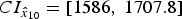 $C{I_{{{\hat x}_{10}}}} = [1586,\;1707.8]$
(respectively
$C{I_{{{\hat x}_{10}}}} = [1586,\;1707.8]$
(respectively
 $C{I_{{{\hat x}_{100}}}} = [1762.6,\;3714.6]$
) when the uncertainty on
$C{I_{{{\hat x}_{100}}}} = [1762.6,\;3714.6]$
) when the uncertainty on
 ${\hat \xi _{MLE}}$
is taken into account, i.e. intervals much larger than those displayed in Table 5.
${\hat \xi _{MLE}}$
is taken into account, i.e. intervals much larger than those displayed in Table 5.
3.2.2. With a fixed dam height
Figure 4 shows the impact on the return level plots of the two interaction laws (and of the deposit shape angle for the volume catch interaction law) for different dam heights and GPD parameterisations. Logically, for both interaction laws, return levels decrease for increasing value of the dam height h d, which simply illustrates the ability of the dam to reduce the hazard in the runout zone. Furthermore, for a fixed GPD parametrisation and dam height, the energy dissipation law generally evaluates a higher return period for a given path abscissa than the volume catch interaction law. This suggests that the dam is more efficient in protecting potential elements at risk under the assumption of a dam/avalanche interaction governed by energy dissipation rather than by volume catch. An exception to this rule, however, is observed for the ‘extreme’ deposit angle shape ϕ = 9° (just below the 10° local slope, which is its maximal possible value), i.e. the case catching the highest volume of snow behind the dam. For instance, in the case where h d = 6 m, ℓd = 100 m and ϕ = 9° (Fig. 4b), all avalanches are stopped by the dam, whereas, with a similar dam height, a few exceedances are still observed with the energy dissipation law. This highlights well the higher flexibility of the volume catch interaction law due to the additional parameter ϕ.

Fig. 4. Runout distance – return period relationships for different dam heights, the two interaction laws and three possible GPD parameterisations provided by the profile likelihood maximisation. Solid line: ξ 0 = −0.3, dashed line: ξ 0 = 0, dotted curve: ξ 0 = 0.3). (a) With the energy dissipation interaction law. (b) With the volume catch interaction law, ℓd = 100 m: (i) ‘intermediate’ case: ϕ = 0° (standard volume storage), and (ii) ‘optimistic’ case: ϕ = 9° (maximal volume storage and, hence, runout shortening with ‘humid’ snow). In that case, for h d = 6 m, all avalanches are stopped by the dam.
Regarding the influence of ξ
0 in Figure 4, the crossing of the different return level plots on the exponential straight line for the same |ξ
0| values occurs for return levels that slightly decrease with the dam height. This traduces that all interaction laws and dam heights impact the scale of the runout distance distribution only:
 ${X_{{\rm sto}{{\rm p}_{{h_{\rm d}}}}}} - {x_{\rm d}} \gt {x_{\rm b}} - {x_{\rm d}}$
remain always GPD distributed with ξ
0 shape parameter whatever the dam height and interaction law considered.
${X_{{\rm sto}{{\rm p}_{{h_{\rm d}}}}}} - {x_{\rm d}} \gt {x_{\rm b}} - {x_{\rm d}}$
remain always GPD distributed with ξ
0 shape parameter whatever the dam height and interaction law considered.
3.3. Residual risk estimates
3.3.1. Influence of the GPD ξ 0 shape parameter
According to Eqn (16), residual risk is a linear function of exceedance probability, so that most noticeable features in residual risk plots directly derive from what is observable on return level plots. For instance, Figure 5 shows the influence of the dam height h d on the risk reduction with a fixed ξ 0 shape parameter, whereas Figure 6 illustrates, with a constant dam height, the influence of the GPD parametrisation, with the ξ 0 parameter taken in the [−0.3, 0.5] interval.

Fig. 5. Residual risk functions with ξ 0 = 0.3 for various dam heights h d with the energy dissipation interaction law (solid curve) and the volume catch interaction law (dashed curve with circles, ℓd = 100 m), (a) intermediate case ϕ = 0° and (b) ‘optimistic case’ ϕ = 9°.

Fig. 6. Residual risk sensitivity to the GPD parametrisation. h 0 = 1m, V = 50 000 m3, ℓd = 100 m, ϕ = 0° and h d = 6 m. (a) Residual risk functions for various ξ 0 values with the energy dissipation interaction law (solid curve) and the volume catch interaction law (dashed curve with circles). (b) Residual risk bounds constructed according to the ξ 0 = {−0.3; −0.1; 0; 0.1; 0.3; 0.5} sample with the two interaction laws. (c) Sensitivity index δ R(x b, h d ) (Eqn (20)) to the runout tail shape as a function of the building position x b for the two interaction laws, ξ 0 = {−0.3; − 0.1; 0; 0.1; 0.3; 0.5}.
In Figure 5, with both interaction laws, the residual risk reduction as a function of the dam height increase is clear, for example, for a building situated at a position corresponding to the centennial runout without a dam (x b = 1718.4 m) and the energy dissipation law, from 74 993 € with no dam to 57 201 € with h d = 1 m, 35 124 € with h d = 3 m and 33 676 € with h d = 5 m.
In Figure 6a, the GPD shape parameter influence is also clear: the Fréchet-type values tested (ξ 0 > 0) provide the lowest residual risk estimates for buildings situated just above the dam abscissa but lead, by far, to the highest risk estimates further down the path, and vice versa for the Weibull-type values (ξ 0 < 0). The exponential case where ξ 0 = 0 provides intermediate residual risk estimates, and, for one given |ξ 0|, all estimates are the same only for the abscissa position at which the Fréchet and Weibull-type return level plots cross the exponential straight line.
Figure 6b summarises, for the same constant dam height and the two interaction laws, the variability of risk estimates towards runout distribution tail types, i.e. in the plausible ξ 0 range [−0.3, 0.5], slightly positive on average. The resulting lower and upper risk bounds may be very valuable insights for practice. For example, for h d = 6 m and the energy dissipation law, the residual risk is estimated to be in the interval [33 180, 37 389] € for a building situated at a position corresponding to the centennial runout without dam (and ξ 0 = 0.3). The width of the inter-bounds interval depends on the position in the path: it is minimal for ‘intermediate’ abscissas where the different risk curves lead to similar estimates, and is much larger when Fréchet/Weibull-type risk estimates strongly diverge.
The δ R(x b, h d ) sensitivity index (Eqn (20)) more quantitatively ascertains the spread of risk bounds towards ξ 0 values. Figure 6c shows that, as a function of building position and interaction law, the relative difference between risk estimates can be as high as 200%. This indicates that considerable errors can be made if the ξ 0 value for which the risk is minimal is chosen instead of the one maximising the risk at the considered abscissa, and vice versa. For each interaction law, δ R(x b, h d ) has two modes as a function of x b. The first (closer to x d) corresponds to the position where Weibull type estimates are the highest with regard to Fréchet-type estimates, and the second mode, further down in the path, to the opposite case. For very high abscissas, all estimates drop to zero, eventually reducing the sensitivity to the runout tail shape. The local minimum between the two modes in δ R(x b, h d ) corresponds to the region in the path previously discussed where all risk estimates are similar (e.g. abscissa where risk lines are crossing in Fig. 6a).
3.3.2. Influence of the interaction law and of the ϕ deposit shape angle
For all dam heights, the energy dissipation interaction law predicts a strong risk reduction with regard to the no-dam case. Residual risk drops sharply for abscissas just above the dam and this effect is all the more marked when the dam is high. With a standard deposit shape angle ϕ = 0°, the volume catch interaction law predicts a much weaker risk reduction for a given dam height, with residual risk estimates dropping at much lower pace as one goes further down in the path (Fig. 5a). The only exception to the higher efficiency of the energy dissipation interaction law occurs for ‘extremal’ volume storages, for example, with ϕ = 9° in Figure 5b. In that case, with moderate dam heights (1–3 m), the two interaction laws lead to rather similar risk estimates and, for h d = 6 m, the volume catch interaction law predicts an even higher risk reduction since all avalanches are stopped before or at the dam abscissa. As a consequence, in general, for a given abscissa in the path, low and high risk bounds obtained towards possible runout tails are much higher for a given dam height with the volume catch law than with the energy dissipation law (Fig. 6b). Also the pattern in resulting sensitivity index is shifted to the right with the volume catch interaction law, with higher values further down in the path (Fig. 6c).
To further quantify the effect of ϕ on the risk estimation, Figure 7 systematically investigates the h d = 5.5 m and ℓd = 50 m case, which stays within the validity range of the two interaction laws for all ϕ values (for the volume catch interaction law, the limit height is 5.9 m with V = 50 000 m3, ϕ = 9° and ℓd = 50 m). As expected, the residual risk increases when the deposit shape angle becomes increasingly negative and hence, the dam, under the volume catch interaction law, becomes less efficient. For this 5.5 m dam height, for which none of the interaction laws is able to stop all avalanches, the energy dissipation interaction law remains the most optimistic regarding the beneficial action of the dam. Risk estimates provided by the volume catch interaction law become close to the energy dissipation law only with the maximal ϕ = 9° value, and much higher with ‘less optimistic’ lower deposit shape angles (Fig. 7a).

Fig. 7. Residual risk sensitivity to the interaction law, with focus on the ϕ deposit shape angle: ℓd = 50 m, ξ 0 = 0.3 and h d = 5.5 m. (a) Residual risk function according to various deposit shape angles ϕ (volume catch interaction law). For comparison, the residual risk with the energy dissipation interaction law is plotted as a solid curve with squares. The dam construction cost C 0 h d is the black dashed horizontal line. (b) Residual risk bounds constructed according to the ϕ = {−40°; −20°; 0°; 3°; 6°; 9°} sample (volume catch interaction law), (i) without or (ii) with the energy dissipation interaction law. The dam construction cost C 0 h d is the black dashed horizontal line. (c) Sensitivity index to the interaction law δ′ R(x b, h d ) (Eqn (23)) as a function of the building position x b without or with the energy dissipation interaction law, ϕ = {−40°; −20°; 0°; 3°; 6°; 9°}.
From the set of risk curves of Figure 7a, for each position in the path, two risk bound couples can be built: the first considers the minimum and maximum risk estimates with the volume catch interaction law according to the variability on ϕ only (Fig. 7b(i)).The second takes into account, in addition, the minimal risk value provided by the energy dissipation interaction law (Fig. 7b(ii)). In other words, due to the higher efficiency postulated by the energy dissipation law, upper risk bounds are the same in the two cases, whereas lower bounds differ sightly. For example, without considering the energy dissipation law, the residual risk is estimated to be in the interval [35 172, 104 233] € for a building situated at a position corresponding to the centennial runout without dam (with ξ 0 = 0.3). With the inclusion of the energy dissipation law in the bounds definition, it is in the interval [31 808, 104 233] €.
The resulting sensitivity to the interaction law index δ′ R(x b, h d ) (Eqn (23)) evaluated all over the runout zone ascertains that a maximal error of 130% (including the energy dissipation law)/105% (with the volume catch interaction law only) can be made on the risk quantification if the interaction law chosen is wrong in terms of postulated mechanism and/or deposit shape angle. As for the sensitivity to the GPD parametrisation, the width between these risk bounds and hence the δ′ R(x b, h d ) sensitivity index is small for buildings very close to the dam (highly exposed), as well as very far down in the path (positions reached by the most extreme avalanches only). Sensitivity to interaction law is therefore maximal for buildings situated at ‘intermediate’ abscissa positions (Fig. 7c).
3.4. Optimal dam heights
3.4.1. Influence of the shape parameter ξ
Since the building position in the risk minimisation is fixed, four positions are chosen: the minimal and the maximal decennial and centennial abscissas provided by these possible parameterisations without dam, that is to say {1600 m, 1690.6 m, 1718.4 m, 1765.2 m}. For these, Figure 8 shows the obtained residual risk curves, as functions of the dam height h d, with the energy dissipation law. For each curve, the optimal height minimising the risk is highlighted. It is more or less clear, depending on the abscissa position x b and the ξ 0 value considered, that a minimum can well be found on the range of h d values allowed by the positivity constraint. As intuitively expected, optimal dam heights are higher for buildings situated closer to the dam than for buildings located further down in the path, since it is economically more sound to protect more exposed elements at risk. Also, for very high dam heights, the risk converges to the construction cost C 0 h d. This occurs as soon as the dam is high enough to stop all avalanches before the considered building abscissa, making the additional construction effort unnecessary. The same evaluation can be done considering the volume catch interaction law instead of the energy dissipation law. At this stage, we consider ϕ = 9°, ℓd = 100 m and V = 50 000 m3, i.e. parameter values for which the dam is ‘efficient’ so that it is easier to determine optimal heights minimising the residual risk. This is not always the case with this interaction law (next subsection).

Fig. 8. Optimal design with the energy dissipation law for different GPD parametrisations and at diffent building abscissas x b: (a) 1600 m, (b) 1690.6 m, (c) 1718.4 m, (d) 1765.2 m. Red circles denote the minimum of each residual risk curve. The dashed black line is the asymptotic dam construction cost C 0 h d. The decisional model parameters impose h d ≤ 7.14 m.
Table 6 summarises optimal dam heights and associated risk estimates
 $R({x_{\rm b}},\;h_{\rm d}^{\ast} )$
for the two interaction laws. At first glance it appears that Fréchet like positive ξ
0 values lead to higher optimal heights and higher corresponding minimum estimates in comparison with those using Weibull- or Gumbell-like ξ
0 values. This conclusion reflects the fact that heavy tailed GPD distributions forecast more extreme avalanches than the two other tail types. This makes higher constructions economically advantageous, but the remaining risk after dam construction still higher. Note that the increase with ξ
0 is very clear with the energy dissipation interaction law, and somewhat less clear with the volume catch interaction law. This is attributable to the fact that with the advantageous volume catch parameters used here, low dam heights are already quite efficient. For instance, the 4.18 m limit height is sufficient to stop all avalanches, and it is economically sound to construct up to this height for many of the ξ
0 and x
b values tested.
$R({x_{\rm b}},\;h_{\rm d}^{\ast} )$
for the two interaction laws. At first glance it appears that Fréchet like positive ξ
0 values lead to higher optimal heights and higher corresponding minimum estimates in comparison with those using Weibull- or Gumbell-like ξ
0 values. This conclusion reflects the fact that heavy tailed GPD distributions forecast more extreme avalanches than the two other tail types. This makes higher constructions economically advantageous, but the remaining risk after dam construction still higher. Note that the increase with ξ
0 is very clear with the energy dissipation interaction law, and somewhat less clear with the volume catch interaction law. This is attributable to the fact that with the advantageous volume catch parameters used here, low dam heights are already quite efficient. For instance, the 4.18 m limit height is sufficient to stop all avalanches, and it is economically sound to construct up to this height for many of the ξ
0 and x
b values tested.
Table 6. Optimal dam height
 $h_{\rm d}^{\ast} $
and corresponding minimum risk
$h_{\rm d}^{\ast} $
and corresponding minimum risk
 $R({x_{\rm b}},\;h_{\rm d}^{\ast} )$
with the two interaction laws at the four abscissas x
b = {1600 m, 1690.6 m, 1718.4 m, 1765.2 m}
$R({x_{\rm b}},\;h_{\rm d}^{\ast} )$
with the two interaction laws at the four abscissas x
b = {1600 m, 1690.6 m, 1718.4 m, 1765.2 m}

The parameters are ℓd = 100 m and ϕ = 9°. With these, the maximal dam height is 7.14 m with the energy dissipation law and 4.18 m with the volume catch one.
To confirm this shape parameter effect, previous calculations were generalized, with the energy dissipation law, to a large range of building positions (Fig. 9) and to a quasi continuous sample of ξ
0 values (Fig. 10), retaining in each case
 $h_{\rm d}^{\ast} $
and
$h_{\rm d}^{\ast} $
and
 $R({x_{\rm b}},\;h_{\rm d}^{\ast} )$
. Overall, results illustrate very clearly that, for a given building position, the higher ξ
0, the higher the optimal dam height and corresponding minimum risk. It also appears that the differences in optimal dam heights and corresponding residual risks obtained with different ξ
0 values strongly increase with increasingly high x
b positions up to very high x
b values. For example, Figure 9a illustrates the results of the optimisation procedure all along the path with a typical Fréchet-type choice (ξ
0 = 0.3) the symmetrical Weibull-type choice (ξ
0 = −0.3) and the intermediate Gumbel-type case (ξ
0 = 0). Fréchet-type optimal heights and corresponding risks estimates are systematically higher than Gumbel-type ones, themselves systematically higher than the Weibull-type ones, and these differences increase with x
b. The same conclusions still hold with the volume catch interaction law, even if the decreasing pattern is weaker (Fig. 9b). Difference in tail types especially affects the most extreme return levels and as a consequence, the design choices controlled by these. Note however that for x
b values so high that they are ‘never’ reached by avalanches, the optimal height and the associated residual risk logically drop to zero. This occurs for lower x
b abscissas when ξ
0 is low (e.g. ξ
0 < 0.1) than when ξ
0 is high (e.g. ξ
0 ≥ 0.1) in our range (Fig. 10).
$R({x_{\rm b}},\;h_{\rm d}^{\ast} )$
. Overall, results illustrate very clearly that, for a given building position, the higher ξ
0, the higher the optimal dam height and corresponding minimum risk. It also appears that the differences in optimal dam heights and corresponding residual risks obtained with different ξ
0 values strongly increase with increasingly high x
b positions up to very high x
b values. For example, Figure 9a illustrates the results of the optimisation procedure all along the path with a typical Fréchet-type choice (ξ
0 = 0.3) the symmetrical Weibull-type choice (ξ
0 = −0.3) and the intermediate Gumbel-type case (ξ
0 = 0). Fréchet-type optimal heights and corresponding risks estimates are systematically higher than Gumbel-type ones, themselves systematically higher than the Weibull-type ones, and these differences increase with x
b. The same conclusions still hold with the volume catch interaction law, even if the decreasing pattern is weaker (Fig. 9b). Difference in tail types especially affects the most extreme return levels and as a consequence, the design choices controlled by these. Note however that for x
b values so high that they are ‘never’ reached by avalanches, the optimal height and the associated residual risk logically drop to zero. This occurs for lower x
b abscissas when ξ
0 is low (e.g. ξ
0 < 0.1) than when ξ
0 is high (e.g. ξ
0 ≥ 0.1) in our range (Fig. 10).

Fig. 9. Optimal design sensitivity to the runout tail shape. ℓd = 100 m, ϕ = 9°. (a) Optimal height
 ${h_{\rm d}} = h_{\rm d}^{\ast} $
(dashed curve) and corresponding minimum residual risks
${h_{\rm d}} = h_{\rm d}^{\ast} $
(dashed curve) and corresponding minimum residual risks
 $R({x_{\rm b}},\;h_{\rm d}^{\ast} )$
(solid curves) as functions of the building position x
b with the energy dissipation interaction law. (b) Optimal height
$R({x_{\rm b}},\;h_{\rm d}^{\ast} )$
(solid curves) as functions of the building position x
b with the energy dissipation interaction law. (b) Optimal height
 ${h_{\rm d}} = h_{\rm d}^{\ast} $
(dashed curves) and corresponding minimum residual risk
${h_{\rm d}} = h_{\rm d}^{\ast} $
(dashed curves) and corresponding minimum residual risk
 $R({x_{\rm b}},\;h_{\rm d}^{\ast} )$
(solid curves) as functions of the building position x
b with the volume catch interaction law. (c) Risk sensitivity index
$R({x_{\rm b}},\;h_{\rm d}^{\ast} )$
(solid curves) as functions of the building position x
b with the volume catch interaction law. (c) Risk sensitivity index
 ${\delta _{R({x_{\rm b}},\;h_{\rm d}^{\ast} )}}$
(Eqn (22)) as function of the optimal design sensitivity index
${\delta _{R({x_{\rm b}},\;h_{\rm d}^{\ast} )}}$
(Eqn (22)) as function of the optimal design sensitivity index
 ${\delta _{{x_{\rm b}},\;h_{\rm d}^{\ast}}} $
(Eqn (21)) for the two interaction laws. Each point of the plot corresponds to a different building abscissa x
b. Black dashed line is the first bisector of the scatter plot.
${\delta _{{x_{\rm b}},\;h_{\rm d}^{\ast}}} $
(Eqn (21)) for the two interaction laws. Each point of the plot corresponds to a different building abscissa x
b. Black dashed line is the first bisector of the scatter plot.

Fig. 10. Optimal dam height (a) and corresponding minimum risk estimate (b) as continuous functions of the GPD shape parameter ξ 0 and building position x b, energy dissipation law. (a) Optimal dam height. (b) Risk value at the optimal dam height.
In terms of optimal design sensitivity indexes
 ${\delta _{{x_{\rm b}},\;R(h_{\rm d}^{\ast} )}}$
and
${\delta _{{x_{\rm b}},\;R(h_{\rm d}^{\ast} )}}$
and
 ${\delta _{{x_{\rm b}},\;h_{\rm d}^{\ast}}} $
, values lower than for the risk sensitivity indexes δ
R(x
b,
h
d
)
and δ′
R(x
b,
h
d
)
are obtained. Still, they remain quite high, up to 120% with the energy dissipation law and 40% with the volume catch interaction law, depending on the x
b position (Fig. 9c). Hence, optimal dam heights and associated minimum risk estimates can be badly appraised, by a factor two if a wrong ξ
0 value is considered, for instance at high (obviously, not too high to be unattainable) abscissas in the path, where the sensitivity to the tail behaviour is the highest. Finally the scatter plot of the two indexes (Fig. 9c) shows that the ξ
0 choice is slightly more influential on the optimal design than on the corresponding risk estimate, but this effect is not very marked.
${\delta _{{x_{\rm b}},\;h_{\rm d}^{\ast}}} $
, values lower than for the risk sensitivity indexes δ
R(x
b,
h
d
)
and δ′
R(x
b,
h
d
)
are obtained. Still, they remain quite high, up to 120% with the energy dissipation law and 40% with the volume catch interaction law, depending on the x
b position (Fig. 9c). Hence, optimal dam heights and associated minimum risk estimates can be badly appraised, by a factor two if a wrong ξ
0 value is considered, for instance at high (obviously, not too high to be unattainable) abscissas in the path, where the sensitivity to the tail behaviour is the highest. Finally the scatter plot of the two indexes (Fig. 9c) shows that the ξ
0 choice is slightly more influential on the optimal design than on the corresponding risk estimate, but this effect is not very marked.
3.4.2. Influence of the interaction law
Figure 11 shows the residual risk curves as a function of the dam height h
d for various deposit shape angles. Whereas things were rather simple with the energy dissipation law (Fig. 8), here, as a result of the higher complexity of the volume catch interaction law, many cases are likely to occur. First, green squares (+; Fig. 11) are optimal heights resulting from the positivity constraint in the interaction law. Second, for the abscissa cases of Figures 8b–d, it is observed that, for the lowest deposit shape angles tested, the risk curves never stop increasing: the cost of the dam is then always high enough to dominate the total cost. Such curve shapes induce an optimal height equal to zero (black asterisk; *; Fig. 11), which never occured for the same abscissas with the energy dissipation law (Fig. 8). Third, red dots (
 $ \bullet $
; Fig. 11) denote ‘true’ optimal heights resulting from the residual risk minimisation on a dam height range where the risk derivative exists. Finally, for highly negative deposit shape angles and low abscissas in the path (− 40° and − 20°; Fig. 11a), the risk decreases over a very large h
d range and the maximal value allowed by the positivity constraint is very high. In that cases, we have stopped the analysis at 30 m, assuming that higher dams would not be allowed for environmental or technical reasons, even if they would apparently be sound from a purely economical perspective. Such limits, rather than true optimal dam heights, are all equal to 30 m. They appear as black triangles (#; Fig. 11).
$ \bullet $
; Fig. 11) denote ‘true’ optimal heights resulting from the residual risk minimisation on a dam height range where the risk derivative exists. Finally, for highly negative deposit shape angles and low abscissas in the path (− 40° and − 20°; Fig. 11a), the risk decreases over a very large h
d range and the maximal value allowed by the positivity constraint is very high. In that cases, we have stopped the analysis at 30 m, assuming that higher dams would not be allowed for environmental or technical reasons, even if they would apparently be sound from a purely economical perspective. Such limits, rather than true optimal dam heights, are all equal to 30 m. They appear as black triangles (#; Fig. 11).

Fig. 11. Optimal design with the volume catch interaction law for different deposit shape angles and at different building abscissas x b: (a) 1600.0 m, (b) 1690.6 m, (c) 1718.4 m, (d) 1765.2 m. The dashed black line is the asymptotic dam construction cost C 0 h d. Particular decisional model parameters are ℓd = 100 m, ξ 0 = 0.3. The positivity constraint depends on the considered deposit shape angle ϕ, but is not very restrictive for low deposit shape angles, e.g h d ≤ 34.5 m for ϕ = −40°, h d ≤ 13.3 m for ϕ = 0° and h d ≤ 4.18 m for ϕ = 9°. When the maximal dam height allowed by the interaction law is above 30 m, the numerical minimum search is restricted to the [0, 30] interval. Symbology regarding the different residual risk minima refers to the different optimum types pointed out in the Appendix and is detailed in the text (Section: ‘Influence of the interaction law’).
To fully quantify the sensitivity of the optimal design and corresponding minimum risk estimate to the interaction law, Figure 12 spans a large set of building positions and deposit shape angles with the deposit volume interaction law, and the energy dissipation law is also considered. Figure 12a shows that with the deposit volume interaction law, for each deposit shape angle ϕ, an abscissa x
b in the path can be found where the optimal dam height drops brutally from a high
 $h_{\rm d}^{\ast} $
value to zero, whereas the residual risk switches to the baseline risk without the dam. This behaviour comes from the fact that, with the deposit volume interaction law, for high abscissas, strictly increasing risk curves are always obtained where the dam construction cost dominates the risk reduction due to the dam protective effect. The path position at which this optimal height drops to zero is observed to decrease with ϕ, since a lower value of ϕ implies a less efficient dam.
$h_{\rm d}^{\ast} $
value to zero, whereas the residual risk switches to the baseline risk without the dam. This behaviour comes from the fact that, with the deposit volume interaction law, for high abscissas, strictly increasing risk curves are always obtained where the dam construction cost dominates the risk reduction due to the dam protective effect. The path position at which this optimal height drops to zero is observed to decrease with ϕ, since a lower value of ϕ implies a less efficient dam.

Fig. 12. Optimal design sensitivity to interaction law, ℓd = 100 m, ξ
0 = 0.3. (a) Optimal height
 ${h_{\rm d}} = h_{\rm d}^{\ast} $
(dashed line) and corresponding minimum residual risk
${h_{\rm d}} = h_{\rm d}^{\ast} $
(dashed line) and corresponding minimum residual risk
 $R({x_{\rm b}},\;h_{\rm d}^{\ast} )$
(solid line) as functions of the building position x
b with different interaction laws: energy dissipation and volume catch with various deposit shape angles. (b) Optimal dam height as continuous function of the abscissa x
b and of the deposit shape angle ϕ. The black area is the region where no optimal design exists.
$R({x_{\rm b}},\;h_{\rm d}^{\ast} )$
(solid line) as functions of the building position x
b with different interaction laws: energy dissipation and volume catch with various deposit shape angles. (b) Optimal dam height as continuous function of the abscissa x
b and of the deposit shape angle ϕ. The black area is the region where no optimal design exists.
More generally, Figure 12a confirms that, for a given GPD parametrisation, when the optimal dam height exists, except for the highest ϕ value tested, it is higher with the volume catch interaction law than with the energy dissipation law, and that the corresponding remaining risk is higher as well. These effects are due to the generally lower risk reduction for a given dam height with the volume catch interaction law, except when ϕ is close to its maximal possible value. This is all the more true when ϕ is low, making the dam less efficient. For example, at the centennial abscissa x b = 1718.4 m (ξ 0 = 0.3), optimal heights and corresponding minimum risk are 0 m (no optimum) and 75 800 € (baseline risk) with ϕ = −40°, 10.6 m and 59 500 € respectively, and 4.6 m and 30 300 € with the energy dissipation law. In contrast, for ϕ = 9°, optimal height (4.18 m) and corresponding risk (23 100 €) are lower than with the energy dissipation law, since the limit height that stops all avalanches is reached.
Finally, Figure 12b shows the spread of the optimal dam height, when it exists, as a continuous function of the deposit shape angle and the building position, with, as written above, a maximal optimal dam height set to 30 m. For low deposit shape angles, say ϕ< − 10°, this maximal 30 m value is easily attained, but as the dam is weakly useful, it is rapidly (i.e. when one goes down in the path) observed that no protection is economically more advantageous than a huge dam. This (black; Fig. 12b) no-optimum domain, where the best economical choice is h d = 0 m, begins at abscissa 1625 m for ϕ = −40°, at abscissa 1662 m for ϕ = −20° and at abscissa 1677 m for ϕ = −10°. For higher deposit shape angles, the no optimum area becomes increasingly narrower, and the maximal optimal height decreases. As a limit case, for ϕ = 9°, the optimal height exists all over the investigated x b range, but it is very small (4.18 m, as written above, even smaller than the optimal height provided by the energy dissipation law at the same abscissa).
This lastly illustrates the higher complexity of the volume catch interaction law. With the energy dissipation law, high optimal dam heights are found for abscissa positions close to the dam and, the higher the dam, the higher its efficiency in reducing the risk, so that
 $h_{\rm d}^{\ast} $
smoothly tends to zero with x
b. In contrast, with the volume catch interaction law,
$h_{\rm d}^{\ast} $
smoothly tends to zero with x
b. In contrast, with the volume catch interaction law,
 $h_{\rm d}^{\ast} $
is controlled primarily by ϕ rather than by x
b. Low values close or equal to the limit value due to the positivity constraint correspond to the highest ϕ value and the risk reduction is important, whereas very high
$h_{\rm d}^{\ast} $
is controlled primarily by ϕ rather than by x
b. Low values close or equal to the limit value due to the positivity constraint correspond to the highest ϕ value and the risk reduction is important, whereas very high
 $h_{\rm d}^{\ast} $
values can be obtained over a large range of positions in the path for low ϕ values. The dam is then rather inefficient in reducing risk, but still economically sound, before rapidly dropping to zero as soon as construction is no longer justified.
$h_{\rm d}^{\ast} $
values can be obtained over a large range of positions in the path for low ϕ values. The dam is then rather inefficient in reducing risk, but still economically sound, before rapidly dropping to zero as soon as construction is no longer justified.
4. DISCUSSION AND CONCLUSION
4.1. Summary of the work done and possible extension
In snow avalanche long-term forecasting, existing risk and optimal design methods are computationally intensive and, therefore rarely used in a real engineering context. In addition, they ground on discussible assumptions for hazard modelling, for instance, regarding the distribution of extreme runouts, and their interaction with defense structures. In this work, we addressed these limitations by expanding a pre-existing quasi analytical decisional model (Eckert and others, Reference Eckert, Parent, Faug and Naaim2008) to make it usable with much wider classes of avalanche runout models based on extreme value statistics and of avalanche/defense structure interaction laws.
Specifically, we replaced the classical exponential runout model by the more general Generalized Pareto model. Coupled with a Poisson model for occurrences, the Pareto model has theoretical justifications that promote its use for modelling ‘all’ possible tails of distributions. This is a huge advantage that should make it sufficient for determining high return period events and perform risk and optimal design computations on most of the avalanche paths. Indeed, whereas the exponential distribution may fit runout data on runout zones having a regular topography compatible with a light tail behaviour only, the GPD distribution may cope also for bounded or heavy tailed runout distance distributions controlled by more complex/irregular topographies. However, when the runout zone topography is really extravagant, even the GPD may fail, and a statistical-numerical approach should be prefered (Section 4.4, below).
Regarding the defense structure, a simple flow-dam law based on local dissipation of kinetic energy was compared with a more flexible law based on the volume stored upstream of the dam. The energy dissipation interaction law provides a formula linking the runout distance in the path without a dam to the runout with a dam of height h d, depending on only the height of the flow h 0. The volume catch interaction law provides the same output, but depending on the deposit volume upstream the dam and on the total volume of the avalanche. Intricately, the stored volume value of V obs(h d) not only depends on the dam height but also on the dam width and on the shape angle of the deposit upstream the dam. It is noted that, as reported in Figure 1, the deposit shape angle can be related either to the humidity rate of the snow, the velocity of the avalanche and/or the μ frictional effect. As a consequence, the volume catch interaction law is more flexible, allowing a more insightful inclusion of the avalanche behaviour one considers the analysis.
Combining these elementary steps, we have obtained simple risk formulae to quantify risk and perform the optimal design of an avalanche dam in a quick and efficient way that covers a variety of situations corresponding to different path topographies (tail types) and/or types of snow (deposit shape angles). From these, we showed how a detailed uncertainty propagation and sensitivity study (data quantity, stochastic avalanche modelling and flow/obstacle interaction assumptions) can be conducted, leading to intervals and bounds for risk estimates and optimal design choices. Practical implementation has been made on a typical case study from the French Alps, illustrating the approach and allowing us to more broadly discuss and evaluate the sensitivity of risk quantification and minimisation procedures for avalanche hazard modelling choices.
A somewhat criticisable point of the approach is that we used an extremely rough quantification of the costs. We did this to obtain analytical equations of the dam height and the stochastic hazard model. In fact, analytical solutions exist as soon as the residual risk can be written as:
 $$R({x_{\rm b}},{h_{\rm d}}) = {C_0}({h_{\rm d}}) + {k_{\rm p}} \times p\left( {{X_{{\rm sto}{{\rm p}_{{h_{\rm d}}}}}} \gt {x_{\rm b}}} \right),$$
where k p is a proportionality coefficient. Hence, the approach works as soon as the damage is supposed not to vary with avalanche intensity (pressure, flow depth, etc.). In Eqn (16), we considered the worst-case: k p = C 1 Aλ, i.e. a total C 1 loss as soon as the building of value C 1 at the abscissa x b is attained. This is compatible with an economical point of view saying that a building loses all of its value as soon as it has been hit one time by an avalanche because nobody will be ready to buy it afterwards. More generally, it may provide a useful upper bound to stand within full approximation.
However, implementing other choices more compatible with data regarding damages by avalanches to various types of constructions is straightforward, for example,
 ${k_{\rm p}} = A\lambda {C_1}\overline {\cal V} $
with
${k_{\rm p}} = A\lambda {C_1}\overline {\cal V} $
with
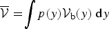 $\overline {\cal V} = \!{\int} p(y){{\cal V}_{\rm b}}(y)\;{\rm d}y$
the average vulnerability towards the whole range of avalanche intensities that can be derived from the vulnerability curves of, for example, Favier and others (Reference Favier, Bertrand, Eckert and Naaim2014a). In practice,
$\overline {\cal V} = \!{\int} p(y){{\cal V}_{\rm b}}(y)\;{\rm d}y$
the average vulnerability towards the whole range of avalanche intensities that can be derived from the vulnerability curves of, for example, Favier and others (Reference Favier, Bertrand, Eckert and Naaim2014a). In practice,
 $\overline {\cal V} $
may be roughly in the [0.05, 0.5] interval, depending on the considered building technology and local hazard distribution, leading to residual risk estimates systematically lower than those provided by our worst case approach.
$\overline {\cal V} $
may be roughly in the [0.05, 0.5] interval, depending on the considered building technology and local hazard distribution, leading to residual risk estimates systematically lower than those provided by our worst case approach.
Also, the A actualisation factor was used to obtain finite total risk estimates on the long range, but there is nothing against working at the annual timescale instead, as often done in risk assessment methods in the snow avalanche field (e.g. Keylock and others, Reference Keylock, McClung and Magnusson1999). This only requires transforming the total construction cost C 0(h d) into an annual construction cost C′0(h d) = C 0(h d)/A. This shows that the actualisation factor is interpretable, with our simple risk/costs expression, as an amortising period for our dam.
Eventually, Eqn (24) highlights well that the approach, even if originally designed as individual-risk based (Arnalds and others, Reference Arnalds, Jonasson and Sigurdsson2004), should rather be seen as ‘local-risk’ based: risk is evaluated and minimised with regard to the abscissa x b, without considering elements at risk possibly located at other positions in the path, but with possible consideration of many elements at risk together at the abscissa x b as soon as they can be combined into a single C 1 value. For instance, here, only damages to a building were studied, but similar computations could easily be performed with furniture or even humans inside the building that would be considered as elements at risk. For the latter, recent developments relating lethality rates to avalanche impacts could be used (Favier and others, Reference Favier, Eckert, Bertrand and Naaim2014b). However, this would also imply monetising human life, and we prefer to avoid this ethically contestable issue at this stage.
4.2. Main findings of the sensitivity analysis
Despite the theoretical interest of the GPD distribution with regard to simpler distributions (modelling ‘all’ possible tails of extreme avalanche runouts), the case study has shown the difficulty to practically fit it on real runout data. Specifically, it was impossible to obtain a realistic shape parameter estimate by simply maximising the likelihood of the data sample at hand. We strongly believe that this may occur more often than not for avalanche runout data. Since the shape parameter is specifically the one that fully determines the tail behaviour type (Fréchet, Gumbel or Weibull), this may cause huge miss-specification of high return levels, and therefore induce a bad assessment of the related risk. Here, we have proposed a practical way to tackle the difficulty: implement a profile likelihood maximisation method, given a reasonable set of possible shape parameters containing the different tail types (for our case study, [−0.3, 0.5], with a preferred value ξ 0 = 0.3), and consider the whole range of return level plots this set leads to within a sensitivity analysis in (residual) risk estimation and optimal design of a defense structure. Also, for the defense structure effect, it is, in practice, not easy to make a single choice between the two we considered and, for the deposit volume one, to select which deposit shape angle/snow type should be preferred. Furthermore, it can even be reasonably argued that risk mapping/defense structure design should be efficient according to all possible interaction processes/laws, so that making land use planning decisions on the basis of one single snow type may be contested. We therefore addressed this question as well within the sensitivity analysis, with the goal of having a comprehensive picture of the sensitivity to the different assumptions made in hazard modelling (the way the flow interacts with the structure is included in the hazard modelling).
In summary, the risk sensitivity to the GPD shape parameter was assessed as being a bit more influential with regard to the interaction law choice: up to 200% relative error according to Eqn (20), versus up to 130% relative error according to Eqn (23). However, these sensitivity indexes are both very high, and of the same order of magnitude. We conclude that the statistical distribution of runouts (and, e.g. the tail type), as well as the interaction law, are both important if one wants to properly estimate the residual risk in the runout zone according to a given dam height. In addition, the two sensitivity indexes δ R(x b, h d ) (Eqn (20)) and δ′ R(x b, h d ) (Eqn (23)) showed more (the former) or less (the latter) complex behaviours according to the abscissa position in the path, but both took their highest values for abscissa positions of interest for hazard mapping/zoning procedures. Indeed, modelling assumptions, for instance the tail behaviour, most strongly affect high magnitude events but become insignificant at abscissa almost never reached by avalanches. As a consequence, the very high sensitivity to hazard modelling assumptions we have highlighted may well be critical in practice for engineers and stakeholders concerned with land-use planning decisions. This is a good argument to recommend the bounds approach we have proposed instead of working on the basis of a single estimate that may be far from the true risk.
Then, a sensitivity study was conducted for the decisional procedure. Here also, sensitivity to the ξ
0 GPD shape parameter choice has been shown to be high whatever the considered interaction law. For instance, the higher ξ
0, the higher the optimal height, and the higher the remaining residual risk after the dam construction. Furthermore, we highlighted that the sensitivity to ξ
0 measured by the decisional sensitivity indexes
 ${\delta _{{x_{\rm b}},\;h_{\rm d}^{\ast}}} $
(Eqn (21)) and
${\delta _{{x_{\rm b}},\;h_{\rm d}^{\ast}}} $
(Eqn (21)) and
 ${\delta _{{x_{\rm b}},\;R(h_{\rm d}^{\ast} )}}$
(Eqn (22)) is also especially high (up to
${\delta _{{x_{\rm b}},\;R(h_{\rm d}^{\ast} )}}$
(Eqn (22)) is also especially high (up to
 $120\% $
) for buildings situated far down in the path, but still sometimes reached by avalanches. Regarding the sensitivity of the optimal design procedure to the interaction law choice, it was first shown that the volume catch interaction law has a less stable behaviour than the energy dissipation law, because of its higher number of parameters and more complex dependency on h
d. Hence, the higher flexibility of the volume catch law and especially, its ability to better reflect the variability of the nature of the flowing snow, has a practical drawback: the optimal design procedure is more difficult to carry out, with different cases needing to be carefully accounted for.
$120\% $
) for buildings situated far down in the path, but still sometimes reached by avalanches. Regarding the sensitivity of the optimal design procedure to the interaction law choice, it was first shown that the volume catch interaction law has a less stable behaviour than the energy dissipation law, because of its higher number of parameters and more complex dependency on h
d. Hence, the higher flexibility of the volume catch law and especially, its ability to better reflect the variability of the nature of the flowing snow, has a practical drawback: the optimal design procedure is more difficult to carry out, with different cases needing to be carefully accounted for.
Meanwhile, it was possible to show that the lower the deposit shape angle ϕ, the higher the optimal dam height, when it exists, but the higher the residual risk after the dam construction. This simply comes from the fact that the lower the deposit shape angle one considers, the less efficient the dam is in reducing the risk. Because of this effect, for nearly all possible ϕ values,
 $h_{\rm d}^{\ast} $
is a strongly discontinuous function of x
b. The position in the path beyond which an optimal height no longer exists increases with the deposit shape angle, until disappearing (on the range of reasonable building positions x
b considered) for the maximal possible value ϕ = 9°. For the latter, the dam is the most efficient, making its construction nearly always rewarded by a cost reduction up to, for example, 4.18 m for ℓd = 100 m, the limit value that stops everything. It is the only deposit volume interaction law parametrisation for which a given dam height is more efficient in reducing the risk than with the energy dissipation law. For all other ϕ values tested, and whatever the position in the path, the optimal height (when it exists) and the remaining risk are higher with the volume catch law.
$h_{\rm d}^{\ast} $
is a strongly discontinuous function of x
b. The position in the path beyond which an optimal height no longer exists increases with the deposit shape angle, until disappearing (on the range of reasonable building positions x
b considered) for the maximal possible value ϕ = 9°. For the latter, the dam is the most efficient, making its construction nearly always rewarded by a cost reduction up to, for example, 4.18 m for ℓd = 100 m, the limit value that stops everything. It is the only deposit volume interaction law parametrisation for which a given dam height is more efficient in reducing the risk than with the energy dissipation law. For all other ϕ values tested, and whatever the position in the path, the optimal height (when it exists) and the remaining risk are higher with the volume catch law.
All in all, risk and optimal design sensitivity to hazard modelling assumptions regarding the behaviour of extreme runout and the perturbation of the flow by a permanent defense structures seem to be both very strong. Even if more case studies may be needed to be fully affirmative, this may well be true for a large variety of avalanche paths, and even for a range of defense structure and flow/structure interaction processes much wider than those considered in this study. It is a very important outcome for practice, which somewhat differs from what is observed regarding sensitivity to vulnerability/costs. Indeed, according to theoretical (Abraham and Cadre, Reference Abraham and Cadre2004) and practical (Favier and others, Reference Favier, Eckert, Bertrand and Naaim2014b) evidence, rough vulnerability/cost estimates may be sufficient to determine the defense structure that minimises the risk even if the true risk is then badly estimated. Here, in contrast, we have shown that both risk and optimal design evaluations will fail in producing sensible results if hazard modelling assumptions are even slightly fallacious.
4.3. Modelling variability and uncertainty in risk and optimal design procedures
The sensitivity/uncertainty analysis has been carried out through various methods. First, a classical uncertainty propagation approach has been implemented to derive confidence intervals for high-return levels from the Poisson-GPD point estimates and the related standard errors. We have adapted two approaches to our profile likelihood context and shown that, for it, the deviance-based approach may be the most robust. Second, we considered a reduced range of ξ
0 values and, conditional to these, plugged the point estimates for the other Poisson-GPD model parameters provided by the profile likelihood maximisation in the residual risk functions. At this stage, we ignored the data quantity related uncertainty (parameter standard errors), focusing on the sensitivity to ξ
0 in risk and optimal design approaches through the indexes δ
R(x
b, h
d),
 ${\delta _{{x_{\rm b}},\;h_{\rm d}^{\ast}}} $
and
${\delta _{{x_{\rm b}},\;h_{\rm d}^{\ast}}} $
and
 ${\delta _{R({x_{\rm b}},\;h_{\rm d}^{\ast} )}}$
.
${\delta _{R({x_{\rm b}},\;h_{\rm d}^{\ast} )}}$
.
Yet, such a two-step approach is somewhat contestable, since it is conceptually more satisfactory to take the parameter uncertainty in account into the sensitivity analysis. A possible way to achieve this would be to switch to a Bayesian approach, averaging the residual risk functions over the posterior distribution of model parameters and evaluating the optimal dam heights and sensitivity indexes accordingly. Conditionally upon ξ 0, the approach could have been partly implemented analytically thanks to conjugation properties (Parent and Bernier, Reference Parent and Bernier2003a, Reference Parent and Bernierb). However, residual risk functions would then have been no longer fully explicit, which is the main reason we preferred working under the classical paradigm in this work. Furthermore, the limitation of working conditionally upon ξ 0 thus would have remained. As a consequence, the real added value of a further non-analytical Bayesian consideration of the problem is probably to work with informative priors on all GPD parameters, for instance ξ. To construct them, one could use the results reported in the literature regarding the tail behaviour of avalanche runouts in other areas/paths (with care since the result of a presumable Fréchet-type tail behaviour obtained for our case study contradicts the evidences of a Weibull type behaviour obtained on larger samples; Keylock (Reference Keylock2005); Ancey (Reference Ancey2012)). This extra-data information would be of great help in practice, avoiding the ξ 0 choice we had to make because of our limited dataset and, presumably reducing the width of high-return level confidence intervals. However, in that case, there would clearly be no full analytical solution of the problem, since no conjugate distribution exists for ξ.
Regarding the interaction law choice, we proceeded as for ξ 0 (sensitivity index δ′ R(x b, h d ) ), but things are a little bit different. Clearly, here, one deals not with uncertainty related to a limited data sample, but with a real modelling assumption regarding the type of dam/flow interaction and consecutive deposit shape angle. Hence, what should be done in practice with the high-sensitivity highlighted remains a difficult question: for example, to always choose the energy dissipation one, no matter what the rheological behaviour it hides, because it is the most stable numerically? Or to take a mean or a maximum value provided by each of the interaction laws so as to maximise the safety with the final decision? If some expert information about the most probable amount and type of snow and hence, deposit shape angle, is available, the volume catch interaction law is probably a good option. However, this is clearly not often the case. To help the engineer, Appendix pushes forward the comparison between the two interaction laws we used. Also, in practice, we clearly recommend testing both and interpret results in terms of sensitivity/bounds as introduced in this work.
Finally, we kept constant the (linear) cost model and the avalanche size parameters required for both interaction laws. This was done to reduce complexity, and focus on the interaction law and GPD shape influence. Simple/plausible forms/values were chosen, which should guarantee the overall robustness of our results. Yet, it cannot be excluded that for specific forms/values very different from ours, different outcomes in terms of residual risk and optimal design behaviour and sensitivity could be obtained. This remains to be investigated in further work.
4.4. Other outlooks for further work
Even if extreme value statistics are used, for example, in the different variations of the runout ratio approach, for example, McClung (Reference McClung2000, Reference McClung2001), our feeling is that, for snow avalanche problems, their use would probably be more intense than is currently the case. By replacing the exponential distribution with the much more general GPD one, our work may contribute to the diffusion of important extreme value concepts such as the tail behaviour in this specific community. However, much work on this question remains to be done, for instance, to more deeply analyse extreme runouts on data samples as large and clean as possible within this framework. In the extreme value community, optimal design approaches in which real efforts on costs and decision modelling are made remain, to our knowledge, seldom (e.g. Rietsch and others, Reference Rietsch, Naveau, Gilardi and Guillou2013), and our work may encourage further developments in this promising direction.
Second, the bridge needs to be made between similar risk and optimal design approaches involving an avalanche numerical propagation model (Barbolini and others, Reference Barbolini, Cappabianca and Savi2004a; Cappabianca and others, Reference Cappabianca, Barbolini and Natale2008; Eckert and others, Reference Eckert, Parent, Faug and Naaim2009; Favier and others, Reference Favier, Eckert, Bertrand and Naaim2014b). Since with these, the expected damage can easily be computed according to existing vulnerability curves and the multivariate avalanche model outputs, they have the advantage of avoiding the assumptions we have made regarding a constant loss, whatever the avalanche impact on a considered element at risk. Also, they are able to deal with the most complex path topographies on which runout extrapolation beyond the furthest recorded value will fail, even with a GPD tail. On the other hand, whether such statistical-numerical approaches have desirable extreme value properties (tail behaviour, etc.), which could be crucial for well evaluating the most damageable events, remains a critical and open question. Also, clearly, their inherent computational cost will remain an obstacle to their use in engineering practice, which justifies the development of simpler alternatives such as ours.
Finally, avalanches/defense structure interaction remains a research field of high practical relevance, very active, but also in which much work remains to be done to better understand the complex physics it involves. However, it will be clearly useful to expand our work to other types of defence structures and avalanche flow interaction laws already available. For instance, it must be remembered that the two we considered correspond to idealised cases only (typical but limited Froude number ranges). Hence, first ideal candidates to enlarge the applicability of our approach are interaction laws combining runout shortening by energy dissipation and volume catch. Such laws account for both the storage effects and the local dissipation of kinetic energy and are therefore able to work at intermediate Froude numbers (Faug, Reference Faug2004). Potentially, they could be implemented within the same framework, making the results of the risk and optimal design computations less specific to one type of flow/obstacle interaction (and/or to one given snow type), which would in turn facilitate the engineer's choice. However, if the convenience of having analytical risk equations at hand remains, it is still worth investigation.
ACKNOWLEDGEMENTS
We thank the ANR research program MOPERA (Modélisation probabiliste pour l'Étude du Risque d'Avalanche – http://www.avalanches.fr/mopera-projet/) and the MAP3 Alcotra Interreg program for financially supporting this work. Thierry Faug and Mohamed Naaim are grateful to the financial support by the People Programme (Marie Curie Actions) of the European Unions Seventh Framework Programme under REA grant agreement No. 622899 (FP7-PEOPLE-2013-IOF, GRAINPACT).
APPENDIX
EXISTENCE OF OPTIMAL HEIGHTS WITH THE VOLUME CATCH INTERACTION LAW
For the general GPD case, when ξ ≠ 0, the derivative of Eqn (19) with regard to the dam height is:
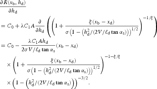 $$\eqalign{& \displaystyle{{\partial R({x_{\rm b}},{h_{\rm d}})} \over {\partial {h_{\rm d}}}} \cr & = {C_0} + \lambda {C_1}A\displaystyle{\partial \over {\partial {h_{\rm d}}}}\left( {{{\left( {1 + \displaystyle{{\xi ({x_{\rm b}} - {x_{\rm d}})} \over {\sigma {{\left( {1 - \left( {{{h_{\rm d}^{\rm 2}} / {(2V/{\ell _{\rm d}}\tan {\alpha _{\rm s}})}}} \right)} \right)}^{1/2}}}}} \right)}^{ - 1/\xi}}} \right) \cr & = {C_0} - \displaystyle{{\lambda {C_1}A{h_{\rm d}}} \over {2\sigma V/{\ell _{\rm d}}\tan {\alpha _{\rm s}}}}({x_{\rm b}} - {x_{\rm d}}) \cr & \quad \times {\left( {1 + \displaystyle{{\xi ({x_{\rm b}} - {x_{\rm d}})} \over {\sigma {{\left( {1 - \left( {{{h_{\rm d}^{\rm 2}} / {(2V/{\ell _{\rm d}}\tan {\alpha _{\rm s}})}}} \right)} \right)}^{1/2}}}}} \right)^{ - 1 - \xi /\xi}} \cr & \quad \times {\left( {1 - \left( {{{h_{\rm d}^{\rm 2}} / {(2V/{\ell _{\rm d}}\tan {\alpha _{\rm s}})}}} \right)} \right)^{ - 3/2}}.} $$
This expression allows better understanding of the different cases likely to occur. Figures 13a, b shows the no optimum case, where the risk derivative is positive all over the range of possible h d values and, hence, the residual risk is a strictly increasing function of h d. This is typically observed for buildings situated at large abscissas in the path and/or for low values of the deposit shape angle ϕ. According to the volume catch interaction law, the dam has then a very small protective effect, so that the loss reduction with increasing h d values is always lower than the concomitant construction cost increase.

Fig. 13. Existence of optimal heights with the volume catch interaction law, ξ 0 = 0.3. (a) Derivative plot and (b) Risk plot for the no optimum case: The used parameter set is: ϕ = −40°, ℓd = 50 m and x b = 1690.7 m. (c) Derivative plot and (d) Risk plot for the pseudo-optimum case induced by the positivity constraint in the volume catch interaction law. The damage to the building costs are zero for h d values exceeding the positivity constraint h d = 5.9 m in this case. For higher dams, all avalanches are stopped below or at the dam abscissa and the risk derivative does not exist. The used parameter set is: ϕ = 9°, ℓd = 50 m and x b = 1589.7 m. (e) Derivative plot and (f) Risk plot for the real optimum case corresponding to residual risk minimisation. The used parameter set is: ϕ = 3°, ℓd = 150 m, x b = 1718.7 m.
Figures 13c, d shows the case of a pseudo-optimum due to the positivity constraint in Eqn (11). The risk derivative is always negative over the range of possible h d values, so that the minimum risk obtained corresponds to the maximal investigated h d value. This is typically observed for buildings situated just beyond the dam abscissa in the path and/or for high values of the deposit shape angle ϕ. The dam has then a very high-protective efficiency, making the additional construction effort rewarded all over the possible h d range. Noteworthy, the maximal investigated height is, in this case, h d = (V × 2tan (α s)/ℓd)1/2, the limit value just sufficient to stop all avalanches before the considered element at risk. From a practical point of view, this height can be considered an optimal choice.
Finally, Figures 13e, f shows the case of a real optimum occurring on the investigated h d range. In fact, the residual risk derivative has even two zeros in this case, but only the one corresponding to the local minimum of the residual risk function is of interest. It highlights the dam height above which the additional protective effect no longer compensates the additional construction costs (in this case to the limit height stopping all avalanches below the element at risk). This is typically observed for reasonable building positions/deposit shape angles, intermediate between the two extreme cases previously discussed.
CONFIDENCE INTERVALS FOR RETURN LEVELS WITH PROFILE LIKELIHOOD GPD ESTIMATES
With the delta method
According to Eqn (4), the σ, ξ and λ derivatives of the return level x T (the indices ‘stop’ and ‘0’ are dropped in the return level, for simplicity, and so is the x T >x d condition) are, respectively:
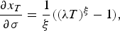 $$\displaystyle{{\partial {x_T}} \over {\partial \sigma}} = \displaystyle{1 \over \xi} ((\lambda T{)^\xi} - 1),$$
 $$\displaystyle{{\partial {x_T}} \over {\partial \xi}} = - \displaystyle{\sigma \over {{\xi ^2}}}((\lambda T{)^\xi} - 1) + \displaystyle{\sigma \over \xi} {(\lambda T)^\xi} \ln (\lambda T)),$$
 $$\displaystyle{{\partial {x_T}} \over {\partial \lambda}} = \sigma {T^\xi} {(\lambda )^{\xi - 1}}.$$
In our profile-likelihood approach, we set the ξ
0 value, and determine
 $\hat \sigma ({\xi _0})$
, which yields:
$\hat \sigma ({\xi _0})$
, which yields:
 $${\hat x_T}({\xi _0}) = {x_T}({\xi _0},\hat \sigma ({\xi _0}),\hat \lambda ) = {x_{\rm d}} + \displaystyle{{\hat \sigma ({\xi _0})} \over {{\xi _0}}}((\hat \lambda T{)^{{\xi _0}}} - 1).$$
The delta method considers
 ${\hat x_T}$
to be asymptotically normally distributed (theorem 2.4 of Coles, Reference Coles2001). In our case, this writes:
${\hat x_T}$
to be asymptotically normally distributed (theorem 2.4 of Coles, Reference Coles2001). In our case, this writes:
 $${\hat x_T}({\xi _0}){\rm : \;} N({x_T}({\xi _0},\hat \sigma ({\xi _0}),\hat \lambda ),{V_{{x_T}}}({\xi _0})),$$
where
 ${V_{{x_T}}}({\xi _0}) = \nabla x_T^T ({\xi _0}){V_{\sigma ({\xi _0}),\lambda}} \nabla {x_T}({\xi _0})$
. V
σ(ξ
0), λ
is the approximate variance-covariance matrix of the profile likelihood estimates and
${V_{{x_T}}}({\xi _0}) = \nabla x_T^T ({\xi _0}){V_{\sigma ({\xi _0}),\lambda}} \nabla {x_T}({\xi _0})$
. V
σ(ξ
0), λ
is the approximate variance-covariance matrix of the profile likelihood estimates and
 $$\nabla {x_T}({\xi _0}) = \left( {\matrix{ {\displaystyle{{\partial {x_T}({\xi _0})} \over {\partial \sigma}}} \cr {\displaystyle{{\partial {x_T}({\xi _0})} \over {\partial \lambda}}} \cr}} \right)$$
is evaluated at
 $(\hat \sigma ({\xi _0}),\hat \lambda )$
. It follows that an approximate (1 − α) confidence interval for x
T
(ξ
0) is:
$(\hat \sigma ({\xi _0}),\hat \lambda )$
. It follows that an approximate (1 − α) confidence interval for x
T
(ξ
0) is:
 $${\hat x_T}({\xi _0}) \pm {z_{\alpha /2}}\sqrt {{V_{{x_T}}}({\xi _0})}, $$
where z α/2 is the (1 − (α/2)) quantile of the standard normal distribution.
On the basis of the deviance statistics
The deviance statistics defined in Section 2 in the context of the GPD – exponential model choice, allows us to obtain another confidence interval for high-return levels. In our case, one needs to evaluate the profile deviance at the ξ 0 value. To do so, according to Eqn (4), for ξ 0 ≠ 0, we can write σ(ξ 0) = ξ 0(x T (ξ 0) − x d )/(λT)(ξ 0 ) − 1. Replacing all occurrences of σ in the log-likelihood function by this expression leads to the searched profile deviance as a function of ξ 0, λ and x T (ξ 0). According to theorem 2.5 of Coles, Reference Coles2001, its asymptotic distribution is again, the one degree of freedom χ 2 distribution, which provides the search for (1 − α) confidence interval for the true value of x T (ξ 0), with α the considered significance level.
Figure 14 applies this result to the evaluation of the 95% confidence interval for the centennial runout. The best guess
 ${\hat x_{100}}$
is at the minimum of the profile log-likelihood. The cut-off straight line corresponds to
${\hat x_{100}}$
is at the minimum of the profile log-likelihood. The cut-off straight line corresponds to
 $(1/2)\chi _1^2 (0.05) = 1.921$
. Its intersections with the profile log–likelihood corresponds to the bounds of the searched 95% confidence interval. Note that these are nonsymmetric around the best guess
$(1/2)\chi _1^2 (0.05) = 1.921$
. Its intersections with the profile log–likelihood corresponds to the bounds of the searched 95% confidence interval. Note that these are nonsymmetric around the best guess
 ${\hat x_{100}}$
, an important difference from the delta method, where the asymptotic normality assumption imposes symmetry of confidence intervals on return levels.
${\hat x_{100}}$
, an important difference from the delta method, where the asymptotic normality assumption imposes symmetry of confidence intervals on return levels.

Fig. 14. Deviance based 95% confidence interval (CI) for the 100 a return level, ξ 0 = 0.3. The green square denotes the minimum of the negative log-likelihood curve. The red line is the χ2 based 95% threshold. Its intersection with the negative log likelihood curve delimitates the 95% confidence interval for the centennial runout distance.
IS IT POSSIBLE TO FURTHER COMPARE THE TWO FLOW/DAM INTERACTION LAWS?
It is tempting to push forward the direct comparison between the two flow/dam interaction laws used in the present paper. By considering n = 1/2 (confined zone upstream of the dam) and by making use of Taylor expansion, the volume's catch interaction (Eqn (10)) law yields:
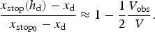 $$\displaystyle{{{x_{{\rm stop}}}({h_{\rm d}}) - {x_{\rm d}}} \over {{x_{{\rm sto}{{\rm p}_{\rm 0}}}} - {x_{\rm d}}}} \approx 1 - \displaystyle{1 \over 2}\displaystyle{{{V_{\rm obs}}} \over {{V}}}. $$
The avalanche volume and the volume stored upstream of the dam can be expressed respectively as:
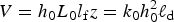 $V = {h_0}{L_0}{l_{\rm f}}z = {k_0}h_0^2 {\ell _{\rm d}}$
and V
obs = k
s
Lℓd
h
d, under the assumption of a rough proportionality for the avalanche length L
0 = k
0
h
0, with L the deposit length and k
s a coefficient representing the deposit shape. This leads to
$V = {h_0}{L_0}{l_{\rm f}}z = {k_0}h_0^2 {\ell _{\rm d}}$
and V
obs = k
s
Lℓd
h
d, under the assumption of a rough proportionality for the avalanche length L
0 = k
0
h
0, with L the deposit length and k
s a coefficient representing the deposit shape. This leads to
 $$\displaystyle{{{x_{{\rm stop}}}({h_{\rm d}}) - {x_{\rm d}}} \over {{x_{{\rm sto}{{\rm p}_{\rm 0}}}} - {x_{\rm d}}}} \approx 1 - \displaystyle{1 \over 2}\displaystyle{{{k_{\rm s}}L{h_{\rm d}}} \over {{k_0}h_0^2}}. $$
By making use of k s = 1 and L = h d/(2tan(α s)) (triangular-shaped deposit upstream of the dam), we have:
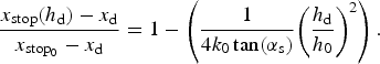 $$\displaystyle{{{x_{{\rm stop}}}({h_{\rm d}}) - {x_{\rm d}}} \over {{x_{{\rm sto}{{\rm p}_{\rm 0}}}} - {x_{\rm d}}}} = 1 - \left( {\displaystyle{1 \over {4{k_0}\tan ({\alpha _{\rm s}})}}{{\left( {\displaystyle{{{h_{\rm d}}} \over {{h_0}}}} \right)}^2}} \right).$$
This equation is equivalent to the linear model (Eqn (9)) only if:
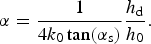 $$\alpha = \displaystyle{1 \over {4{k_0}\tan ({\alpha _{\rm s}})}}\displaystyle{{{h_{\rm d}}} \over {{h_0}}}.$$
For this latter equation to be true, either the right-hand side term must be kept constant or α must be a function of h d/h 0. The first option leads to a somewhat non-physical result: the length of the deposit and the volume stored upstream of the dam are constant whatever the dam height. The second option can give more physical results, but only with small values of α, 10 times smaller than the typical value of 0.14 that was used in this study. This factor 10 explains why the volume's catch law generally evaluates a residual risk higher than that obtained with the energy dissipation law, as discussed in the present paper.
More generally, this second option also shows that the two interaction laws are definitely different models, difficult to directly compare. For instance, the run-out shortening derived from the Taylor's expansion of the volume's catch law is no longer a linear function of h d/h 0. However, better understanding the similarities and differences between the two interaction laws we considered may make it possible in the future to better describe flows characterised by intermediate Froude numbers, in links with the more general formulations previously advocated that combines the two shortening processes (Faug, Reference Faug2004). This may be important since the 1–5 Froude range, to which neither of our two interaction laws is perfectly adapted, is typical for snow avalanche flows in many paths.


 Open access