


1. Introduction
The entrainment hypothesis is the standard turbulence closure used in integral descriptions of turbulent jets and plumes. It links the entrainment velocity, the rate at which ambient fluid is entrained into the plume, to a typical velocity inside the plume by a single coefficient of proportionality
 ${\it\alpha}$
, the entrainment coefficient. For axisymmetric releases, the entrainment hypothesis takes the form (Turner Reference Turner1986)
${\it\alpha}$
, the entrainment coefficient. For axisymmetric releases, the entrainment hypothesis takes the form (Turner Reference Turner1986)
 $$\begin{eqnarray}-(ru)_{r=\infty }={\it\alpha}\hat{r}{\hat{w}},\end{eqnarray}$$
where
 $r$
and
$r$
and
 $u$
denote the radial direction and radial velocity, and
$u$
denote the radial direction and radial velocity, and
 $\hat{r}$
and
$\hat{r}$
and
 ${\hat{w}}$
are the characteristic plume radius and velocity respectively. The entrainment coefficient
${\hat{w}}$
are the characteristic plume radius and velocity respectively. The entrainment coefficient
 ${\it\alpha}$
is generally the only parameter representing the effect that turbulence has on the mean flow, and it is remarkable that the behaviour of a flow as complex as a turbulent plume can be captured by a closure as simple as (1.1). In this respect it could be regarded as the free-shear equivalent of the quadratic friction relation for wall-bounded flows under fully rough conditions, which links the wall shear stress to the free-stream velocity via a single friction coefficient.
${\it\alpha}$
is generally the only parameter representing the effect that turbulence has on the mean flow, and it is remarkable that the behaviour of a flow as complex as a turbulent plume can be captured by a closure as simple as (1.1). In this respect it could be regarded as the free-shear equivalent of the quadratic friction relation for wall-bounded flows under fully rough conditions, which links the wall shear stress to the free-stream velocity via a single friction coefficient.
The value of
 ${\it\alpha}$
is subject to significant variability: typical values for the ‘top-hat’ entrainment coefficient are in the range
${\it\alpha}$
is subject to significant variability: typical values for the ‘top-hat’ entrainment coefficient are in the range
 $0.065<{\it\alpha}<0.080$
in jets and
$0.065<{\it\alpha}<0.080$
in jets and
 $0.10<{\it\alpha}<0.16$
in pure plumes (Fischer et al.
Reference Fischer, List, Koh, Imberger and Brooks1979; Carazzo, Kaminski & Tait Reference Carazzo, Kaminski and Tait2006). Here, the term ‘top-hat’ refers to a description that assumes a uniform value of profiles of velocity and buoyancy over a finite radius. The flux-balance parameter
$0.10<{\it\alpha}<0.16$
in pure plumes (Fischer et al.
Reference Fischer, List, Koh, Imberger and Brooks1979; Carazzo, Kaminski & Tait Reference Carazzo, Kaminski and Tait2006). Here, the term ‘top-hat’ refers to a description that assumes a uniform value of profiles of velocity and buoyancy over a finite radius. The flux-balance parameter
 ${\it\Gamma}$
(Morton Reference Morton1959), which will be rigorously defined in § 2, allows one to distinguish between jets and pure plumes. In neutrally stratified environments, vertically (denoted
${\it\Gamma}$
(Morton Reference Morton1959), which will be rigorously defined in § 2, allows one to distinguish between jets and pure plumes. In neutrally stratified environments, vertically (denoted
 $z$
) oriented flows evolve in such a way that
$z$
) oriented flows evolve in such a way that
 ${\it\Gamma}(z)$
either remains constant or approaches an asymptotic limit. For a pure jet, which has no buoyancy,
${\it\Gamma}(z)$
either remains constant or approaches an asymptotic limit. For a pure jet, which has no buoyancy,
 ${\it\Gamma}(z)=0$
. Plumes that have an excess of momentum at their source are called ‘forced’, and
${\it\Gamma}(z)=0$
. Plumes that have an excess of momentum at their source are called ‘forced’, and
 ${\it\Gamma}$
is in the range
${\it\Gamma}$
is in the range
 $0<{\it\Gamma}<1$
; plumes that have a deficit of momentum at their source are called ‘lazy’, and have
$0<{\it\Gamma}<1$
; plumes that have a deficit of momentum at their source are called ‘lazy’, and have
 ${\it\Gamma}>1$
(Hunt & Kaye Reference Hunt and Kaye2005). Both forced and lazy plumes will transition to a pure plume (
${\it\Gamma}>1$
(Hunt & Kaye Reference Hunt and Kaye2005). Both forced and lazy plumes will transition to a pure plume (
 ${\it\Gamma}=1$
) as the flow develops. A review of jets and plumes can be found in, e.g., Hunt & van den Bremer (Reference Hunt and van den Bremer2011).
${\it\Gamma}=1$
) as the flow develops. A review of jets and plumes can be found in, e.g., Hunt & van den Bremer (Reference Hunt and van den Bremer2011).
There is significant variation in
 ${\it\alpha}$
between different experiments, as is evident from the large range of observed values. This can be attributed to differences in experimental set-ups, experimental error and uncertainty (Turner Reference Turner1986; Kaminski, Tait & Carazzo Reference Kaminski, Tait and Carazzo2005), and also source conditions (George Reference George, Arndt and George1989; Redford, Castro & Coleman Reference Redford, Castro and Coleman2012). However, it is evident that there is a systematic difference between the reported value of
${\it\alpha}$
between different experiments, as is evident from the large range of observed values. This can be attributed to differences in experimental set-ups, experimental error and uncertainty (Turner Reference Turner1986; Kaminski, Tait & Carazzo Reference Kaminski, Tait and Carazzo2005), and also source conditions (George Reference George, Arndt and George1989; Redford, Castro & Coleman Reference Redford, Castro and Coleman2012). However, it is evident that there is a systematic difference between the reported value of
 ${\it\alpha}$
for jets and plumes, which suggests a dependence of
${\it\alpha}$
for jets and plumes, which suggests a dependence of
 ${\it\alpha}$
on
${\it\alpha}$
on
 ${\it\Gamma}$
.
${\it\Gamma}$
.
In this paper we consider restrictions imposed upon the entrainment coefficient
 ${\it\alpha}$
by the equation for the mean kinetic energy. We will refer to this restriction as an entrainment relation hereafter. The entrainment relation couples
${\it\alpha}$
by the equation for the mean kinetic energy. We will refer to this restriction as an entrainment relation hereafter. The entrainment relation couples
 ${\it\alpha}$
to various physical processes such as turbulence production and buoyancy effects. We will refer to entrainment models as the closed relations that are obtained once the various coefficients in the entrainment relation are parameterised. The aim of this paper is to provide a hierarchy of energy-consistent entrainment relations that can be used either in a diagnostic mode, clarifying the physics of turbulent entrainment, or in a prognostic mode, leading to entrainment models that can be used for predictive purposes.
${\it\alpha}$
to various physical processes such as turbulence production and buoyancy effects. We will refer to entrainment models as the closed relations that are obtained once the various coefficients in the entrainment relation are parameterised. The aim of this paper is to provide a hierarchy of energy-consistent entrainment relations that can be used either in a diagnostic mode, clarifying the physics of turbulent entrainment, or in a prognostic mode, leading to entrainment models that can be used for predictive purposes.
To date, no distinction has been made between an entrainment relation and an entrainment model, perhaps because much of the discussion in the literature has focused on the reconciliation of the plume theories of Morton, Taylor & Turner (Reference Morton, Taylor and Turner1956, MTT) and Priestley & Ball (Reference Priestley and Ball1955, PB). These theories are obtained by integrating the axisymmetric Reynolds-averaged Navier–Stokes equations across a plane perpendicular to the mean-flow direction, resulting in a system of coupled ordinary differential equations (ODEs) in terms of integral quantities. The MTT plume equations comprise three ODEs in terms of the volume flux
 $Q$
, the momentum flux
$Q$
, the momentum flux
 $M$
and the buoyancy flux
$M$
and the buoyancy flux
 $F$
. Entrainment into the plume is quantified by a constant parameter
$F$
. Entrainment into the plume is quantified by a constant parameter
 ${\it\alpha}$
(the entrainment coefficient) which features in the volume conservation equation. The PB plume equations consist of three coupled ODEs for
${\it\alpha}$
(the entrainment coefficient) which features in the volume conservation equation. The PB plume equations consist of three coupled ODEs for
 $M$
,
$M$
,
 $F$
and the flux of mean kinetic energy
$F$
and the flux of mean kinetic energy
 $E$
. The PB plume equations rely on a parameterisation of the production of turbulence kinetic energy, or equivalently the Reynolds stress.
$E$
. The PB plume equations rely on a parameterisation of the production of turbulence kinetic energy, or equivalently the Reynolds stress.
A lucid description of how the two models are related was provided by Fox (Reference Fox1970); by simultaneously considering the conservation equations of volume, momentum, buoyancy and mean kinetic energy, he linked the two models and was the first to highlight the constraints imposed on
 ${\it\alpha}$
by the conservation equation for mean kinetic energy, i.e. the entrainment relation. The analysis was restricted to fully self-similar profiles (i.e. the far field), and his model took into account the possibility of the velocity and buoyancy profiles having different widths. Apart from deriving the far-field entrainment relation, Fox derived the PB entrainment model, given by (Fox Reference Fox1970; List & Imberger Reference List and Imberger1973)
${\it\alpha}$
by the conservation equation for mean kinetic energy, i.e. the entrainment relation. The analysis was restricted to fully self-similar profiles (i.e. the far field), and his model took into account the possibility of the velocity and buoyancy profiles having different widths. Apart from deriving the far-field entrainment relation, Fox derived the PB entrainment model, given by (Fox Reference Fox1970; List & Imberger Reference List and Imberger1973)
 $$\begin{eqnarray}{\it\alpha}={\it\alpha}_{j}+({\it\alpha}_{p}-{\it\alpha}_{j}){\it\Gamma},\end{eqnarray}$$
where
 ${\it\alpha}_{j}$
and
${\it\alpha}_{j}$
and
 ${\it\alpha}_{p}$
are the entrainment coefficients for a pure jet and a pure plume respectively. A few years later List & Imberger (Reference List and Imberger1973), starting from the observation that jets and plumes spread at practically the same rate (see also List Reference List1982), derived an entrainment model compatible with (1.2). This is indeed consistent – solutions to the PB model are straight-sided, with identical spreading rate regardless of the value of
${\it\alpha}_{p}$
are the entrainment coefficients for a pure jet and a pure plume respectively. A few years later List & Imberger (Reference List and Imberger1973), starting from the observation that jets and plumes spread at practically the same rate (see also List Reference List1982), derived an entrainment model compatible with (1.2). This is indeed consistent – solutions to the PB model are straight-sided, with identical spreading rate regardless of the value of
 ${\it\Gamma}$
, including forced and lazy plumes (Priestley & Ball Reference Priestley and Ball1955, see also § 5). The PB entrainment model provides predictions for
${\it\Gamma}$
, including forced and lazy plumes (Priestley & Ball Reference Priestley and Ball1955, see also § 5). The PB entrainment model provides predictions for
 ${\it\alpha}$
that are in reasonably good agreement with laboratory experiments on forced plumes in an unstratified ambient (Wang & Law Reference Wang and Law2002; Matulka et al.
Reference Matulka, Lopez, Redondo and Tarquis2014; Ezzamel, Salizzoni & Hunt Reference Ezzamel, Salizzoni and Hunt2015).
${\it\alpha}$
that are in reasonably good agreement with laboratory experiments on forced plumes in an unstratified ambient (Wang & Law Reference Wang and Law2002; Matulka et al.
Reference Matulka, Lopez, Redondo and Tarquis2014; Ezzamel, Salizzoni & Hunt Reference Ezzamel, Salizzoni and Hunt2015).
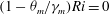
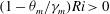
In a response to Fox’s analysis, Morton (Reference Morton1971) highlighted that for a plume rising in a linearly stratified ambient, both models were equally appropriate; however, near the source and the neutral buoyancy level the MTT approach was preferable because it was able to predict plume necking and spreading respectively. Here, necking refers to the observation that lazy plumes tend to contract relatively close to the source (see, e.g., Fannelop & Webber Reference Fannelop and Webber2003), and spreading refers to the widening of a plume once it reaches a location where the buoyancy of the environment is identical to that of the plume (the neutral buoyancy level). Indeed, a problem with (1.2) in stratified environments is that it admits a sign change in
 ${\it\alpha}$
, which motivated the empirical model for the entrainment coefficient proposed by Fischer et al. (Reference Fischer, List, Koh, Imberger and Brooks1979, p. 371). More sophisticated among attempts to model entrainment in plumes is the approach of Telford (Reference Telford1966). Recognising that the assumption of self-similarity is often violated in the context of atmospheric convection, Telford (Reference Telford1966) suggests that the entrainment coefficient is proportional to the turbulence intensity, and solves an additional equation for the turbulence kinetic energy.
${\it\alpha}$
, which motivated the empirical model for the entrainment coefficient proposed by Fischer et al. (Reference Fischer, List, Koh, Imberger and Brooks1979, p. 371). More sophisticated among attempts to model entrainment in plumes is the approach of Telford (Reference Telford1966). Recognising that the assumption of self-similarity is often violated in the context of atmospheric convection, Telford (Reference Telford1966) suggests that the entrainment coefficient is proportional to the turbulence intensity, and solves an additional equation for the turbulence kinetic energy.
Kaminski et al. (Reference Kaminski, Tait and Carazzo2005) should be credited for reintroducing energy-based entrainment relations to the plume literature. Indeed, they built on the foundations laid by Fox (Reference Fox1970), and extended the analysis by relaxing the assumptions regarding the radial profile dependences. This led to an entrainment relation valid for both the near field and the far field, which exposed the physics of entrainment in terms of leading-order quantities. While the main focus of Kaminski et al. (Reference Kaminski, Tait and Carazzo2005) was on turbulent fountains, they argued that the ratio of the width of the velocity profile to the buoyancy (reduced gravity) profile, denoted
 ${\it\lambda}$
, could help to reconcile the spread in
${\it\lambda}$
, could help to reconcile the spread in
 ${\it\alpha}$
for pure plumes. In particular, they showed evidence that small variations of
${\it\alpha}$
for pure plumes. In particular, they showed evidence that small variations of
 ${\it\lambda}$
in the vertical direction had an effect on entrainment, a process they termed similarity drift. A disadvantage of their derivation is the use of top-hat scales for
${\it\lambda}$
in the vertical direction had an effect on entrainment, a process they termed similarity drift. A disadvantage of their derivation is the use of top-hat scales for
 $\hat{r}$
and
$\hat{r}$
and
 ${\hat{w}}$
that depend on the buoyancy flux, which is not standard procedure and is not a logical extension of the scales one defines in jets. This greatly complicates the use of their entrainment relation, as the relation between
${\hat{w}}$
that depend on the buoyancy flux, which is not standard procedure and is not a logical extension of the scales one defines in jets. This greatly complicates the use of their entrainment relation, as the relation between
 ${\it\alpha}$
and the Kaminski entrainment coefficient
${\it\alpha}$
and the Kaminski entrainment coefficient
 ${\it\alpha}_{e}$
is not trivial (see appendix A for details). The framework was further extended with turbulence and pressure contributions by Ezzamel et al. (Reference Ezzamel, Salizzoni and Hunt2015), who provide an entrainment relation directly in terms of the Gaussian entrainment coefficient
${\it\alpha}_{e}$
is not trivial (see appendix A for details). The framework was further extended with turbulence and pressure contributions by Ezzamel et al. (Reference Ezzamel, Salizzoni and Hunt2015), who provide an entrainment relation directly in terms of the Gaussian entrainment coefficient
 ${\it\alpha}_{G}$
. They remark that similarity drift does not feature in
${\it\alpha}_{G}$
. They remark that similarity drift does not feature in
 ${\it\alpha}_{G}$
in the same way as in
${\it\alpha}_{G}$
in the same way as in
 ${\it\alpha}_{e}$
(see also § 3), which, as noted above, is a result of the different scale definitions employed.
${\it\alpha}_{e}$
(see also § 3), which, as noted above, is a result of the different scale definitions employed.
Consideration of a mean energy budget becomes crucial once the restriction of a steady state is lifted. This is because the various profile coefficients characterising the mean and turbulent profiles of velocity and buoyancy play an independent role in defining the structure of the governing integral equations (Craske & van Reeuwijk Reference Craske and van Reeuwijk2015a ,Reference Craske and van Reeuwijk b ). Moreover, a mean kinetic energy equation for unsteady jets and plumes can be readily obtained without significant approximation, thereby circumventing the difficulties that are associated with obtaining a conservation equation for the volume of the plume (see, e.g., Scase & Hewitt Reference Scase and Hewitt2012). Indeed, due to the underlying assumptions, one finds significant differences between existing unsteady plume models (e.g. those of Delichatsios Reference Delichatsios1979; Yu Reference Yu1990; Vul’fson & Borodin Reference Vul’fson and Borodin2001; Scase et al. Reference Scase, Caulfield, Dalziel and Hunt2006), whose properties and consistency can be checked with respect to an overarching framework by appealing to the mean energy equation (Craske & van Reeuwijk Reference Craske and van Reeuwijk2015b ). In the context of entrainment, the use of a momentum–energy framework allows one to deduce that under certain conditions both unsteady jets and plumes remain straight-sided (Craske Reference Craske2015; Craske & van Reeuwijk Reference Craske and van Reeuwijk2015b ), and allowed Craske & van Reeuwijk (Reference Craske and van Reeuwijk2015a ) to obtain a decomposition of the entrainment coefficient for jets, similar to that of Kaminski et al. (Reference Kaminski, Tait and Carazzo2005), but with the important distinction that (1) both turbulence and pressure contributions are included and (2) standard (top-hat) definitions for radius and velocity scales are used.
In § 2, we adapt the momentum–energy framework developed in Craske & van Reeuwijk (Reference Craske and van Reeuwijk2015a
,Reference Craske and van Reeuwijk
b
) to include buoyancy. An entrainment relation that ensures compatibility between volume and energy conservation is derived in § 3, after which a hierarchy of entrainment relations will be provided which naturally accommodate the entrainment relations of Kaminski et al. (Reference Kaminski, Tait and Carazzo2005) and Fox (Reference Fox1970). The implications of the entrainment relation and a physical interpretation are provided in § 4. The entrainment models underlying the MTT and PB theories are discussed in § 5 and an investigation into an appropriate entrainment model for pure jets and pure plumes in an unstratified environment is undertaken in § 6. One of the key requirements in order to systematically study turbulent entrainment is to maintain a constant plume Richardson number
 $\mathit{Ri}$
as the plume ascends; § 7 discusses possibilities of how a constant
$\mathit{Ri}$
as the plume ascends; § 7 discusses possibilities of how a constant
 $\mathit{Ri}$
may be achieved. Concluding remarks are made in § 8.
$\mathit{Ri}$
may be achieved. Concluding remarks are made in § 8.
2. Governing equations
Consider a round high-Reynolds-number turbulent plume orientated in the vertical (
 $z$
) direction whose flow is statistically axisymmetric. We consider Reynolds-averaged conservation equations for volume, streamwise momentum and buoyancy. Adopting the Boussinesq approximation and assuming high-Reynolds-number flow, the governing equations are
$z$
) direction whose flow is statistically axisymmetric. We consider Reynolds-averaged conservation equations for volume, streamwise momentum and buoyancy. Adopting the Boussinesq approximation and assuming high-Reynolds-number flow, the governing equations are
 $$\begin{eqnarray}\displaystyle & \displaystyle \frac{1}{r}\frac{\partial }{\partial r}(r\overline{u})+\frac{\partial \overline{w}}{\partial z}=0, & \displaystyle\end{eqnarray}$$
 $$\begin{eqnarray}\displaystyle & \displaystyle \frac{1}{r}\frac{\partial }{\partial r}(r\overline{u}\,\overline{w}+r\overline{u^{\prime }w^{\prime }})+\frac{\partial }{\partial z}(\overline{w}^{2}+\overline{w^{\prime 2}})=-\frac{\partial \overline{p}}{\partial z}+\overline{b}, & \displaystyle\end{eqnarray}$$
 $$\begin{eqnarray}\displaystyle & \displaystyle \frac{1}{r}\frac{\partial }{\partial r}(r\overline{u}\overline{b}+r\overline{u^{\prime }b^{\prime }})+\frac{\partial }{\partial z}(\overline{w}\overline{b}+\overline{w^{\prime }b^{\prime }})=-N^{2}\overline{w}. & \displaystyle\end{eqnarray}$$
 $(\overline{u},\overline{w})$
correspond to the directions
$(\overline{u},\overline{w})$
correspond to the directions
 $(r,z)$
respectively,
$(r,z)$
respectively,
 $\overline{p}$
denotes the kinematic pressure from which the hydrostatic pressure field resulting from the environmental density
$\overline{p}$
denotes the kinematic pressure from which the hydrostatic pressure field resulting from the environmental density
 ${\it\rho}_{e}(z)$
has been subtracted, and
${\it\rho}_{e}(z)$
has been subtracted, and
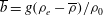 $\overline{b}=g({\it\rho}_{e}-\overline{{\it\rho}})/{\it\rho}_{0}$
is the buoyancy for which
$\overline{b}=g({\it\rho}_{e}-\overline{{\it\rho}})/{\it\rho}_{0}$
is the buoyancy for which
 ${\it\rho}_{0}$
is a reference density. The buoyancy frequency is defined as
${\it\rho}_{0}$
is a reference density. The buoyancy frequency is defined as
 $N^{2}(z)=-(g/{\it\rho}_{0})(\text{d}{\it\rho}_{e}/\text{d}z)$
.
$N^{2}(z)=-(g/{\it\rho}_{0})(\text{d}{\it\rho}_{e}/\text{d}z)$
.
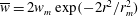
By multiplying (2.2) with
 $2\overline{w}$
, we obtain after some manipulation
$2\overline{w}$
, we obtain after some manipulation
 $$\begin{eqnarray}\displaystyle & & \displaystyle \frac{1}{r}\frac{\partial }{\partial r}(r\overline{u}\,\overline{w}^{2}+2r\overline{u^{\prime }w^{\prime }}\overline{w})+\frac{\partial }{\partial z}(\overline{w}^{3}+2\overline{w^{\prime 2}}\overline{w}+2\overline{p}\,\overline{w})\nonumber\\ \displaystyle & & \displaystyle \quad =2\,\overline{u^{\prime }w^{\prime }}\frac{\partial \overline{w}}{\partial r}+2\,\overline{w^{\prime 2}}\frac{\partial \overline{w}}{\partial z}+2\overline{p}\frac{\partial \overline{w}}{\partial z}+2\overline{w}\overline{b}.\end{eqnarray}$$
This equation will be referred to as the equation of mean kinetic energy, since the typical scale for the mean radial velocity is smaller than the streamwise velocity by a factor
 ${\it\alpha}$
, implying that the mean kinetic energy is dominated by
${\it\alpha}$
, implying that the mean kinetic energy is dominated by
 $\overline{w}^{2}$
. The first two terms of (2.4) represent the radial and vertical transport terms, each containing mean and turbulent flux contributions. The term
$\overline{w}^{2}$
. The first two terms of (2.4) represent the radial and vertical transport terms, each containing mean and turbulent flux contributions. The term
 $2\,\overline{u^{\prime }w^{\prime }}(\partial \overline{w}/\partial r)+2\,\overline{w^{\prime 2}}(\partial \overline{w}/\partial z)$
is associated with the production of turbulence kinetic energy and forms a sink term in the equation for mean kinetic energy. The term
$2\,\overline{u^{\prime }w^{\prime }}(\partial \overline{w}/\partial r)+2\,\overline{w^{\prime 2}}(\partial \overline{w}/\partial z)$
is associated with the production of turbulence kinetic energy and forms a sink term in the equation for mean kinetic energy. The term
 $2\,\overline{p}(\partial \overline{w}/\partial z)$
is a pressure redistribution term and
$2\,\overline{p}(\partial \overline{w}/\partial z)$
is a pressure redistribution term and
 $2\,\overline{w}\overline{b}$
represents the production of mean kinetic energy due to buoyancy. We note that the absence of viscous terms in the equation for mean kinetic energy does not imply that viscous dissipation is neglected altogether. While the viscous dissipation associated with the mean-flow components is indeed negligible at high Reynolds number (
$2\,\overline{w}\overline{b}$
represents the production of mean kinetic energy due to buoyancy. We note that the absence of viscous terms in the equation for mean kinetic energy does not imply that viscous dissipation is neglected altogether. While the viscous dissipation associated with the mean-flow components is indeed negligible at high Reynolds number (
 $\mathit{Re}$
) (see, e.g., Tennekes & Lumley Reference Tennekes and Lumley1972), the component associated with the turbulence cannot be neglected. The latter dissipation rate is crucial in the balance of turbulence kinetic energy, as it is of the same order of magnitude as the turbulence production term (Shabbir & George Reference Shabbir and George1994). However, the balance of turbulence kinetic energy is not considered in this paper, and viscous effects are thus entirely absent from the mathematical description of the mean flow.
$\mathit{Re}$
) (see, e.g., Tennekes & Lumley Reference Tennekes and Lumley1972), the component associated with the turbulence cannot be neglected. The latter dissipation rate is crucial in the balance of turbulence kinetic energy, as it is of the same order of magnitude as the turbulence production term (Shabbir & George Reference Shabbir and George1994). However, the balance of turbulence kinetic energy is not considered in this paper, and viscous effects are thus entirely absent from the mathematical description of the mean flow.
The volume flux
 $Q$
, momentum flux
$Q$
, momentum flux
 $M$
, integral buoyancy
$M$
, integral buoyancy
 $B$
and buoyancy flux
$B$
and buoyancy flux
 $F$
are defined as
$F$
are defined as
 $$\begin{eqnarray}Q\equiv 2\int _{0}^{\infty }\overline{w}r\,\text{d}r,\quad M\equiv 2\int _{0}^{\infty }\overline{w}^{2}r\,\text{d}r,\quad B\equiv 2\int _{0}^{\infty }\overline{b}r\,\text{d}r,\quad F\equiv 2\int _{0}^{\infty }\overline{w}\overline{b}r\,\text{d}r.\end{eqnarray}$$
These integral quantities can be used to define a characteristic plume width, velocity and buoyancy respectively:
 $$\begin{eqnarray}r_{m}\equiv \frac{Q}{M^{1/2}},\quad w_{m}\equiv \frac{M}{Q},\quad b_{m}\equiv \frac{BM}{Q^{2}}.\end{eqnarray}$$
These scales are consistent with top-hat variables; however, it should be noted that the analysis below does not make a priori assumptions regarding the profile shape.
Integration of (2.1)–(2.4) over
 $r$
results in
$r$
results in
 $$\begin{eqnarray}\displaystyle & \displaystyle {\displaystyle \frac{\text{d}Q}{\text{d}z}}=2{\it\alpha}M^{1/2}, & \displaystyle\end{eqnarray}$$
 $$\begin{eqnarray}\displaystyle & \displaystyle {\displaystyle \frac{\text{d}}{\text{d}z}}\left({\it\beta}_{g}M\right)=\frac{FQ}{{\it\theta}_{m}M}, & \displaystyle\end{eqnarray}$$
 $$\begin{eqnarray}\displaystyle & \displaystyle {\displaystyle \frac{\text{d}}{\text{d}z}}\left(\frac{{\it\theta}_{g}}{{\it\theta}_{m}}F\right)=-N^{2}Q, & \displaystyle\end{eqnarray}$$
 $$\begin{eqnarray}\displaystyle & \displaystyle {\displaystyle \frac{\text{d}}{\text{d}z}}\left({\it\gamma}_{g}\frac{M^{2}}{Q}\right)={\it\delta}_{g}\frac{M^{5/2}}{Q^{2}}+2F. & \displaystyle\end{eqnarray}$$
 ${\it\beta}$
,
${\it\beta}$
,
 ${\it\gamma}$
,
${\it\gamma}$
,
 ${\it\theta}$
and
${\it\theta}$
and
 ${\it\delta}$
in (2.7)–(2.10) are profile coefficients associated with the dimensionless momentum flux, energy flux, buoyancy flux and turbulence production respectively. Consistent with Craske & van Reeuwijk (Reference Craske and van Reeuwijk2015a
), the gross value of a profile coefficient, e.g.
${\it\delta}$
in (2.7)–(2.10) are profile coefficients associated with the dimensionless momentum flux, energy flux, buoyancy flux and turbulence production respectively. Consistent with Craske & van Reeuwijk (Reference Craske and van Reeuwijk2015a
), the gross value of a profile coefficient, e.g.
 ${\it\gamma}_{g}$
, is composed of contributions from the mean flow, turbulence and pressure, i.e.
${\it\gamma}_{g}$
, is composed of contributions from the mean flow, turbulence and pressure, i.e.
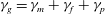 ${\it\gamma}_{g}={\it\gamma}_{m}+{\it\gamma}_{f}+{\it\gamma}_{p}$
. Explicitly, the profile coefficients are defined as
${\it\gamma}_{g}={\it\gamma}_{m}+{\it\gamma}_{f}+{\it\gamma}_{p}$
. Explicitly, the profile coefficients are defined as  $$\begin{eqnarray}\left.\begin{array}{@{}c@{}}\displaystyle {\it\beta}_{m}\equiv \frac{M}{w_{m}^{2}r_{m}^{2}}\equiv 1,\quad {\it\beta}_{f}\equiv \frac{2}{w_{m}^{2}r_{m}^{2}}\int _{0}^{\infty }\overline{w^{\prime 2}}r\,\text{d}r,\quad {\it\beta}_{p}\equiv \frac{2}{w_{m}^{2}r_{m}^{2}}\int _{0}^{\infty }\overline{p}r\,\text{d}r,\\ \displaystyle {\it\gamma}_{m}\equiv \frac{2}{w_{m}^{3}r_{m}^{2}}\int _{0}^{\infty }\overline{w}^{3}r\,\text{d}r,\quad {\it\gamma}_{f}\equiv \frac{4}{w_{m}^{3}r_{m}^{2}}\int _{0}^{\infty }\overline{w}\overline{w^{\prime 2}}r\,\text{d}r,\quad {\it\gamma}_{p}\equiv \frac{4}{w_{m}^{3}r_{m}^{2}}\int _{0}^{\infty }\overline{w}\,\overline{p}r\,\text{d}r,\\ \displaystyle {\it\delta}_{m}\equiv \frac{4}{w_{m}^{3}r_{m}}\int _{0}^{\infty }\overline{w^{\prime }u^{\prime }}{\displaystyle \frac{\text{d}\overline{w}}{\text{d}r}}r\,\text{d}r,\quad {\it\delta}_{f}\equiv \frac{4}{w_{m}^{3}r_{m}}\int _{0}^{\infty }\overline{w^{\prime 2}}{\displaystyle \frac{\text{d}\overline{w}}{\text{d}z}}r\,\text{d}r,\quad {\it\delta}_{p}\equiv \frac{4}{w_{m}^{3}r_{m}}\int _{0}^{\infty }\overline{p}{\displaystyle \frac{\text{d}\overline{w}}{\text{d}z}}r\,\text{d}r,\\ \displaystyle {\it\theta}_{m}\equiv \frac{F}{w_{m}b_{m}r_{m}^{2}},\quad {\it\theta}_{f}\equiv \frac{2}{w_{m}b_{m}r_{m}^{2}}\int _{0}^{\infty }\overline{w^{\prime }b^{\prime }}r\,\text{d}r.\end{array}\right\}\end{eqnarray}$$
It should be noted that the definition of
 ${\it\theta}_{m}$
provides a fundamental relation between the integral buoyancy
${\it\theta}_{m}$
provides a fundamental relation between the integral buoyancy
 $B$
and the buoyancy flux
$B$
and the buoyancy flux
 $F$
as
$F$
as
 $B=FQ/({\it\theta}_{m}M)$
.
$B=FQ/({\it\theta}_{m}M)$
.
The profile coefficients influence the definition of the flux-balance parameter
 ${\it\Gamma}$
, which expresses the ratio of buoyancy force to inertia (Morton Reference Morton1959). As discussed in the introduction,
${\it\Gamma}$
, which expresses the ratio of buoyancy force to inertia (Morton Reference Morton1959). As discussed in the introduction,
 ${\it\Gamma}=0$
for a pure jet and
${\it\Gamma}=0$
for a pure jet and
 ${\it\Gamma}=1$
for a pure plume. In the far field, the first-order (velocity, buoyancy) and second-order (Reynolds stresses, buoyancy variance) statistics are fully self-similar (i.e. preserve shape upon rescaling radius and the quantity in consideration by the local characteristic scales
${\it\Gamma}=1$
for a pure plume. In the far field, the first-order (velocity, buoyancy) and second-order (Reynolds stresses, buoyancy variance) statistics are fully self-similar (i.e. preserve shape upon rescaling radius and the quantity in consideration by the local characteristic scales
 $r_{m}$
,
$r_{m}$
,
 $w_{m}$
and
$w_{m}$
and
 $b_{m}$
), implying that the profile coefficients are therefore constant. In this case, (2.7)–(2.9) are consistent with the classical plume equations
$b_{m}$
), implying that the profile coefficients are therefore constant. In this case, (2.7)–(2.9) are consistent with the classical plume equations
 $$\begin{eqnarray}\displaystyle {\displaystyle \frac{\text{d}Q}{\text{d}z}}=2{\it\alpha}M^{1/2},\quad {\displaystyle \frac{\text{d}M}{\text{d}z}}=\frac{F_{E}Q}{M},\quad {\displaystyle \frac{\text{d}F_{E}}{\text{d}z}}=-N_{E}^{2}Q, & & \displaystyle\end{eqnarray}$$
where
 $F_{E}$
and
$F_{E}$
and
 $N_{E}$
are the effective buoyancy flux and frequency respectively, defined as
$N_{E}$
are the effective buoyancy flux and frequency respectively, defined as
 $$\begin{eqnarray}F_{E}\equiv \frac{F}{{\it\beta}_{g}{\it\theta}_{m}},\quad N_{E}\equiv \frac{N}{\left({\it\theta}_{g}{\it\beta}_{g}\right)^{1/2}}.\end{eqnarray}$$
The connection with the standard plume equations is valuable because these have been widely applied to model problems of further complexity (e.g. the ventilation of buildings; Linden Reference Linden1999). Equation (2.13a,b
) indicates how effects from turbulence (via
 ${\it\beta}_{g}$
) and differences in the shape of the buoyancy and the velocity profiles (via
${\it\beta}_{g}$
) and differences in the shape of the buoyancy and the velocity profiles (via
 ${\it\theta}_{m}$
) influence solutions to the classical plume equations and the practical applications to which they have been applied. For a pure plume in an unstratified environment, the solutions of (2.12a−c
) are the power-law solutions (see, e.g., Turner Reference Turner1979)
${\it\theta}_{m}$
) influence solutions to the classical plume equations and the practical applications to which they have been applied. For a pure plume in an unstratified environment, the solutions of (2.12a−c
) are the power-law solutions (see, e.g., Turner Reference Turner1979)
 $$\begin{eqnarray}Q(z)=\frac{6{\it\alpha}_{p}}{5}M^{1/2}z,\quad M(z)=\left(\frac{9}{10}\right)^{2/3}{\it\alpha}_{p}^{2/3}F_{E}^{2/3}z^{4/3},\quad F_{E}=\text{const.},\end{eqnarray}$$
where
 ${\it\alpha}_{p}$
is the entrainment coefficient for a pure plume. The definition of the flux-balance parameter
${\it\alpha}_{p}$
is the entrainment coefficient for a pure plume. The definition of the flux-balance parameter
 ${\it\Gamma}$
(Morton Reference Morton1959) generalises to
${\it\Gamma}$
(Morton Reference Morton1959) generalises to
 $$\begin{eqnarray}{\it\Gamma}=\frac{5F_{E}Q^{2}}{8{\it\alpha}_{p}M^{5/2}}=\frac{5FQ^{2}}{8{\it\alpha}_{p}{\it\beta}_{g}{\it\theta}_{m}M^{5/2}}=\frac{5}{8{\it\alpha}_{p}{\it\beta}_{g}}\mathit{Ri}.\end{eqnarray}$$
Here, the plume Richardson number
 $\mathit{Ri}$
, representative of the ratio of gravitational to inertial forcing, is defined as
$\mathit{Ri}$
, representative of the ratio of gravitational to inertial forcing, is defined as
 $$\begin{eqnarray}\mathit{Ri}\equiv \frac{b_{m}r_{m}}{w_{m}^{2}}=\frac{FQ^{2}}{{\it\theta}_{m}M^{5/2}}.\end{eqnarray}$$
By construction,
 ${\it\Gamma}=1$
for a pure plume, as is clear from substituting the power-law solution (2.14a,b
) into (2.15). The associated Richardson number is
${\it\Gamma}=1$
for a pure plume, as is clear from substituting the power-law solution (2.14a,b
) into (2.15). The associated Richardson number is
 $\mathit{Ri}_{p}=8{\it\alpha}_{p}{\it\beta}_{g}/5$
; indeed,
$\mathit{Ri}_{p}=8{\it\alpha}_{p}{\it\beta}_{g}/5$
; indeed,
 ${\it\Gamma}$
can be alternatively defined as
${\it\Gamma}$
can be alternatively defined as
 ${\it\Gamma}=\mathit{Ri}/\mathit{Ri}_{p}$
.
${\it\Gamma}=\mathit{Ri}/\mathit{Ri}_{p}$
.
3. The entrainment relation
The system (2.7)–(2.10) comprises four equations with three dependent variables (
 $Q$
,
$Q$
,
 $M$
and
$M$
and
 $F$
) and is thus overdetermined. However, the energy conservation equation (2.4) is derived from, and fully consistent with, the volume and momentum conservation equations (2.1) and (2.2). Integration over the radial direction cannot alter this property, and thus (2.10) must also be fully consistent with (2.7) and (2.8). This places a restriction on
$F$
) and is thus overdetermined. However, the energy conservation equation (2.4) is derived from, and fully consistent with, the volume and momentum conservation equations (2.1) and (2.2). Integration over the radial direction cannot alter this property, and thus (2.10) must also be fully consistent with (2.7) and (2.8). This places a restriction on
 ${\it\alpha}$
, which was introduced into (2.7) by invoking the entrainment hypothesis (1.1).
${\it\alpha}$
, which was introduced into (2.7) by invoking the entrainment hypothesis (1.1).
Using (2.7) as a definition of
 ${\it\alpha}$
and applying the product rule of differentiation to (2.10) and (2.8), it follows that
${\it\alpha}$
and applying the product rule of differentiation to (2.10) and (2.8), it follows that
 $$\begin{eqnarray}\displaystyle {\it\alpha} & \equiv & \displaystyle \frac{1}{2M^{1/2}}{\displaystyle \frac{\text{d}Q}{\text{d}z}}\nonumber\\ \displaystyle & = & \displaystyle \frac{Q}{{\it\beta}_{g}M^{3/2}}\,{\displaystyle \frac{\text{d}}{\text{d}z}}({\it\beta}_{g}M)-\frac{Q^{2}}{2{\it\gamma}_{g}M^{5/2}}{\displaystyle \frac{\text{d}}{\text{d}z}}\left({\it\gamma}_{g}\frac{M^{2}}{Q}\right)+\frac{Q}{2M^{1/2}}{\displaystyle \frac{\text{d}}{\text{d}z}}\left(\log \frac{{\it\gamma}_{g}}{{\it\beta}_{g}^{2}}\right)\nonumber\\ \displaystyle & = & \displaystyle -\frac{{\it\delta}_{g}}{2{\it\gamma}_{g}}+\left(\frac{1}{{\it\beta}_{g}}-\frac{{\it\theta}_{m}}{{\it\gamma}_{g}}\right)\mathit{Ri}+\frac{Q}{2M^{1/2}}{\displaystyle \frac{\text{d}}{\text{d}z}}\left(\log \frac{{\it\gamma}_{g}}{{\it\beta}_{g}^{2}}\right).\end{eqnarray}$$
For an interpretation of the terms in (3.1), see § 4. The entrainment relation (3.1) is a consistency requirement that is valid independently of model choices. This consistency requirement is valuable because entrainment models – which make particular assumptions regarding
 ${\it\beta}_{g}$
,
${\it\beta}_{g}$
,
 ${\it\theta}_{m}$
and
${\it\theta}_{m}$
and
 ${\it\gamma}_{g}$
– have received criticism for not being applicable to specific flows, e.g. for clouds (Squires & Turner Reference Squires and Turner1962) or for reacting plumes (Ricou & Spalding Reference Ricou and Spalding1961; Hermanson & Dimotakis Reference Hermanson and Dimotakis1989). Indeed, the attractiveness of (3.1) is that it is a relation with which all models for entrainment must be consistent. If a particular entrainment model is not in agreement with observations, it therefore becomes a relatively simple matter to pinpoint the cause of the discrepancy. The spreading rate
${\it\gamma}_{g}$
– have received criticism for not being applicable to specific flows, e.g. for clouds (Squires & Turner Reference Squires and Turner1962) or for reacting plumes (Ricou & Spalding Reference Ricou and Spalding1961; Hermanson & Dimotakis Reference Hermanson and Dimotakis1989). Indeed, the attractiveness of (3.1) is that it is a relation with which all models for entrainment must be consistent. If a particular entrainment model is not in agreement with observations, it therefore becomes a relatively simple matter to pinpoint the cause of the discrepancy. The spreading rate
 $\text{d}r_{m}/\text{d}z$
is closely associated with, and is often used to infer,
$\text{d}r_{m}/\text{d}z$
is closely associated with, and is often used to infer,
 ${\it\alpha}$
. It is therefore useful to establish how this quantity can be decomposed:
${\it\alpha}$
. It is therefore useful to establish how this quantity can be decomposed:
 $$\begin{eqnarray}\displaystyle \frac{\text{d}r_{m}}{\text{d}z} & = & \displaystyle \frac{1}{M^{1/2}}\frac{\text{d}Q}{\text{d}z}-\frac{Q}{2M^{3/2}}\frac{\text{d}M}{\text{d}z}\nonumber\\ \displaystyle & = & \displaystyle -\frac{{\it\delta}_{g}}{{\it\gamma}_{g}}+\frac{3}{2}\left(\frac{1}{{\it\beta}_{g}}-\frac{4}{3}\frac{{\it\theta}_{m}}{{\it\gamma}_{g}}\right)\mathit{Ri}+\frac{Q}{M^{1/2}}{\displaystyle \frac{\text{d}}{\text{d}z}}\left(\log \frac{{\it\gamma}_{g}}{{\it\beta}_{g}^{3/2}}\right).\end{eqnarray}$$
Table 1 contains a hierarchy of entrainment relations, which will be detailed below. The entrainment relation (3.1), hereafter called
 ${\it\alpha}$
-F, includes the effects of mean quantities, turbulence and pressure. This entrainment relation makes minimal assumptions about the flow and will form the basis of all simplified entrainment relations described below. It is ideal for use in a diagnostic mode using data obtained from direct simulation, as was done in Craske & van Reeuwijk (Reference Craske and van Reeuwijk2015a
).
${\it\alpha}$
-F, includes the effects of mean quantities, turbulence and pressure. This entrainment relation makes minimal assumptions about the flow and will form the basis of all simplified entrainment relations described below. It is ideal for use in a diagnostic mode using data obtained from direct simulation, as was done in Craske & van Reeuwijk (Reference Craske and van Reeuwijk2015a
).
Table 1. The hierarchy of entrainment relations. These relations are based on an integral or ‘top-hat’ description using definitions (2.5a−d ) and (2.6a−c ); for a conversion to a Gaussian or other description see appendix B.

Table 2. The spreading rate
 $\text{d}r_{m}/\text{d}z$
associated with the entrainment relation. These relations are based on an integral or ‘top-hat’ description using definitions (2.5a−d
) and (2.6a−c
); for a conversion to a Gaussian or other description see appendix B.
$\text{d}r_{m}/\text{d}z$
associated with the entrainment relation. These relations are based on an integral or ‘top-hat’ description using definitions (2.5a−d
) and (2.6a−c
); for a conversion to a Gaussian or other description see appendix B.

Upon making the assumption that
 ${\it\beta}_{g}={\it\beta}_{m}=1$
,
${\it\beta}_{g}={\it\beta}_{m}=1$
,
 ${\it\gamma}_{g}={\it\gamma}_{m}$
and
${\it\gamma}_{g}={\it\gamma}_{m}$
and
 ${\it\delta}_{g}={\it\delta}_{m}$
(i.e. ignoring turbulence and pressure effects), the entrainment relation
${\it\delta}_{g}={\it\delta}_{m}$
(i.e. ignoring turbulence and pressure effects), the entrainment relation
 ${\it\alpha}$
-M, (3.4), is obtained. This is the entrainment relation that was derived by Kaminski et al. (Reference Kaminski, Tait and Carazzo2005), although it is not immediately obvious that
${\it\alpha}$
-M, (3.4), is obtained. This is the entrainment relation that was derived by Kaminski et al. (Reference Kaminski, Tait and Carazzo2005), although it is not immediately obvious that
 ${\it\alpha}$
-M is indeed consistent with their entrainment model; a detailed proof of the equivalence of the two models is provided in appendix A. In contrast to the relation derived by Kaminski et al. (Reference Kaminski, Tait and Carazzo2005), the ‘similarity drift’ term in
${\it\alpha}$
-M is indeed consistent with their entrainment model; a detailed proof of the equivalence of the two models is provided in appendix A. In contrast to the relation derived by Kaminski et al. (Reference Kaminski, Tait and Carazzo2005), the ‘similarity drift’ term in
 ${\it\alpha}$
-M (cf. third term), does not depend on the shape of the buoyancy profile via
${\it\alpha}$
-M (cf. third term), does not depend on the shape of the buoyancy profile via
 ${\it\theta}_{m}$
(see also Ezzamel et al.
Reference Ezzamel, Salizzoni and Hunt2015), but only on
${\it\theta}_{m}$
(see also Ezzamel et al.
Reference Ezzamel, Salizzoni and Hunt2015), but only on
 ${\it\gamma}_{m}$
, i.e. the shape of the velocity profile. The reason for this difference resides in the use of standard top-hat scales in this paper, see appendix A for details. Instead, variations in
${\it\gamma}_{m}$
, i.e. the shape of the velocity profile. The reason for this difference resides in the use of standard top-hat scales in this paper, see appendix A for details. Instead, variations in
 ${\it\theta}_{m}$
influence the second term in
${\it\theta}_{m}$
influence the second term in
 ${\it\alpha}$
-M only, capturing the possible slow variation in the shape of the buoyancy profile discussed in Kaminski et al. (Reference Kaminski, Tait and Carazzo2005). This entrainment relation is ideal for examining the physics of turbulent plumes using experimental data. Indeed, many modern particle image velocimetry and laser Doppler anemometry systems can record high-frequency velocity fields, which, if augmented with appropriate buoyancy measurements, provide access to all of the required coefficients in
${\it\alpha}$
-M only, capturing the possible slow variation in the shape of the buoyancy profile discussed in Kaminski et al. (Reference Kaminski, Tait and Carazzo2005). This entrainment relation is ideal for examining the physics of turbulent plumes using experimental data. Indeed, many modern particle image velocimetry and laser Doppler anemometry systems can record high-frequency velocity fields, which, if augmented with appropriate buoyancy measurements, provide access to all of the required coefficients in
 ${\it\alpha}$
-M. In complexity, the extension of the Kaminski entrainment relation by Ezzamel et al. (Reference Ezzamel, Salizzoni and Hunt2015) sits between
${\it\alpha}$
-M. In complexity, the extension of the Kaminski entrainment relation by Ezzamel et al. (Reference Ezzamel, Salizzoni and Hunt2015) sits between
 ${\it\alpha}$
-F and
${\it\alpha}$
-F and
 ${\it\alpha}$
-M and will not be laboured further here.
${\it\alpha}$
-M and will not be laboured further here.
By assuming full self-similarity in the first- and second-order statistics, and therefore that
 ${\it\beta}_{m}$
,
${\it\beta}_{m}$
,
 ${\it\gamma}_{m}$
and
${\it\gamma}_{m}$
and
 ${\it\delta}_{m}$
are constants, the entrainment relation
${\it\delta}_{m}$
are constants, the entrainment relation
 ${\it\alpha}$
-MS is obtained, see (3.6). Formally, the only strict requirement of obtaining (3.6) from (3.4) is that
${\it\alpha}$
-MS is obtained, see (3.6). Formally, the only strict requirement of obtaining (3.6) from (3.4) is that
 ${\it\gamma}_{m}$
is constant. The relation
${\it\gamma}_{m}$
is constant. The relation
 ${\it\alpha}$
-MS is the entrainment relation derived by Fox (Reference Fox1970), and describes the fundamental connection between the two main unknowns,
${\it\alpha}$
-MS is the entrainment relation derived by Fox (Reference Fox1970), and describes the fundamental connection between the two main unknowns,
 ${\it\delta}_{m}$
and
${\it\delta}_{m}$
and
 ${\it\theta}_{m}$
, and the entrainment coefficient
${\it\theta}_{m}$
, and the entrainment coefficient
 ${\it\alpha}$
. Upon assuming that the profiles are Gaussian and that
${\it\alpha}$
. Upon assuming that the profiles are Gaussian and that
 ${\it\theta}_{m}=1$
, (3.7) is obtained, which will be referred to as
${\it\theta}_{m}=1$
, (3.7) is obtained, which will be referred to as
 ${\it\alpha}$
-MSG. The spreading rate associated with each entrainment relation is presented in table 2. One striking feature of the spreading rate equations is that under the realistic assumption that the far-field behaviour can be described by self-similar Gaussian profiles of equal width (relation
${\it\alpha}$
-MSG. The spreading rate associated with each entrainment relation is presented in table 2. One striking feature of the spreading rate equations is that under the realistic assumption that the far-field behaviour can be described by self-similar Gaussian profiles of equal width (relation
 ${\it\alpha}$
-MSG), the
${\it\alpha}$
-MSG), the
 $\mathit{Ri}$
-term associated with the net effect of buoyancy is identically zero, implying that the spreading rate is determined purely by the profile coefficient associated with the production of turbulence kinetic energy.
$\mathit{Ri}$
-term associated with the net effect of buoyancy is identically zero, implying that the spreading rate is determined purely by the profile coefficient associated with the production of turbulence kinetic energy.
4. Physics of entrainment
In this section, we interpret the physical meaning of the three terms of the entrainment relation. The first term on the right-hand side of (3.3),
 $-{\it\delta}_{g}/(2{\it\gamma}_{g})$
, is the ratio of the dimensionless turbulence production term
$-{\it\delta}_{g}/(2{\it\gamma}_{g})$
, is the ratio of the dimensionless turbulence production term
 ${\it\delta}_{g}$
and the dimensionless energy flux
${\it\delta}_{g}$
and the dimensionless energy flux
 ${\it\gamma}_{g}$
. It should be noted that
${\it\gamma}_{g}$
. It should be noted that
 ${\it\delta}_{g}<0$
under normal circumstances because the production of turbulence kinetic energy is a sink term in the equation for mean kinetic energy (2.10). For jets (
${\it\delta}_{g}<0$
under normal circumstances because the production of turbulence kinetic energy is a sink term in the equation for mean kinetic energy (2.10). For jets (
 $\mathit{Ri}=0$
), this is the only non-zero term in the far field (Craske & van Reeuwijk Reference Craske and van Reeuwijk2015a
). For both pure jets and pure plumes,
$\mathit{Ri}=0$
), this is the only non-zero term in the far field (Craske & van Reeuwijk Reference Craske and van Reeuwijk2015a
). For both pure jets and pure plumes,
 ${\it\delta}_{g}$
is dominated by
${\it\delta}_{g}$
is dominated by
 ${\it\delta}_{m}$
, the other production term
${\it\delta}_{m}$
, the other production term
 ${\it\delta}_{f}$
and pressure redistribution term
${\it\delta}_{f}$
and pressure redistribution term
 ${\it\delta}_{p}$
being comparatively small (Craske Reference Craske2015; Craske & van Reeuwijk Reference Craske and van Reeuwijk2015a
).
${\it\delta}_{p}$
being comparatively small (Craske Reference Craske2015; Craske & van Reeuwijk Reference Craske and van Reeuwijk2015a
).
The second term in (3.3) is the net effect of buoyancy on the entrainment coefficient, which we will discuss in depth in the next paragraphs. The third term is associated with streamwise changes in the shape of the velocity statistics through the profile coefficients
 ${\it\beta}_{g}$
and
${\it\beta}_{g}$
and
 ${\it\gamma}_{g}$
. These quantities are primarily associated with the mean flow, but also contain pressure and turbulence contributions, the latter being known to require a large distance to come to a full equilibrium (Wang & Law Reference Wang and Law2002; Ezzamel et al.
Reference Ezzamel, Salizzoni and Hunt2015). The third term is associated with the similarity drift discussed in Kaminski et al. (Reference Kaminski, Tait and Carazzo2005) and Carazzo et al. (Reference Carazzo, Kaminski and Tait2006), although as previously mentioned the present formulation does not contain contributions of
${\it\gamma}_{g}$
. These quantities are primarily associated with the mean flow, but also contain pressure and turbulence contributions, the latter being known to require a large distance to come to a full equilibrium (Wang & Law Reference Wang and Law2002; Ezzamel et al.
Reference Ezzamel, Salizzoni and Hunt2015). The third term is associated with the similarity drift discussed in Kaminski et al. (Reference Kaminski, Tait and Carazzo2005) and Carazzo et al. (Reference Carazzo, Kaminski and Tait2006), although as previously mentioned the present formulation does not contain contributions of
 ${\it\theta}_{m}$
because of the standard top-hat definitions of
${\it\theta}_{m}$
because of the standard top-hat definitions of
 $r_{m}$
and
$r_{m}$
and
 $w_{m}$
used in this paper (see appendix A).
$w_{m}$
used in this paper (see appendix A).

Figure 1. The far-field entrainment relation
 ${\it\alpha}$
-MS, plotted together with the MTT entrainment model (fixed
${\it\alpha}$
-MS, plotted together with the MTT entrainment model (fixed
 ${\it\alpha}$
; red line) and the PB entrainment model (fixed
${\it\alpha}$
; red line) and the PB entrainment model (fixed
 ${\it\delta}_{m}$
; blue line).
${\it\delta}_{m}$
; blue line).
The entrainment relation
 ${\it\alpha}$
-MS, which assumes full self-similarity and leading-order contributions only, will be used to further interpret the physics of turbulent entrainment. As emphasised earlier, entrainment relations ensure consistency between volume, momentum and energy conservation at the integral level. Figure 1 shows the functional dependence of the entrainment coefficient
${\it\alpha}$
-MS, which assumes full self-similarity and leading-order contributions only, will be used to further interpret the physics of turbulent entrainment. As emphasised earlier, entrainment relations ensure consistency between volume, momentum and energy conservation at the integral level. Figure 1 shows the functional dependence of the entrainment coefficient
 ${\it\alpha}$
on the turbulence production contribution
${\it\alpha}$
on the turbulence production contribution
 $-{\it\delta}_{m}/(2{\it\gamma}_{m})$
and net buoyancy
$-{\it\delta}_{m}/(2{\it\gamma}_{m})$
and net buoyancy
 $(1-{\it\theta}_{m}/{\it\gamma}_{m})\mathit{Ri}$
as a grey isosurface. Only points on this surface are physically realisable; therefore, models of entrainment must necessarily be defined on this surface. Two entrainment models associated with the MTT and PB plume theories, which form the subject of § 5, are shown by red and blue lines respectively. The entrainment relation makes no assumption about how profile coefficients (e.g.
$(1-{\it\theta}_{m}/{\it\gamma}_{m})\mathit{Ri}$
as a grey isosurface. Only points on this surface are physically realisable; therefore, models of entrainment must necessarily be defined on this surface. Two entrainment models associated with the MTT and PB plume theories, which form the subject of § 5, are shown by red and blue lines respectively. The entrainment relation makes no assumption about how profile coefficients (e.g.
 ${\it\delta}_{m}$
,
${\it\delta}_{m}$
,
 ${\it\gamma}_{m}$
) depend on properties of the flow such as the Richardson number
${\it\gamma}_{m}$
) depend on properties of the flow such as the Richardson number
 $\mathit{Ri}$
, source conditions and local environmental conditions, for example. Indeed, the way in which entrainment depends on these aspects of the flow remains an open question, which is partially addressed for flows in an unstratified ambient in § 6. The entrainment relation does, however, impose a fundamental consistency requirement linking the various model parameters, and therefore provides a necessary framework for the investigation of entrainment. In the far field, where profiles are assumed to be fully self-similar, profile coefficients will only depend on
$\mathit{Ri}$
, source conditions and local environmental conditions, for example. Indeed, the way in which entrainment depends on these aspects of the flow remains an open question, which is partially addressed for flows in an unstratified ambient in § 6. The entrainment relation does, however, impose a fundamental consistency requirement linking the various model parameters, and therefore provides a necessary framework for the investigation of entrainment. In the far field, where profiles are assumed to be fully self-similar, profile coefficients will only depend on
 $\mathit{Ri}$
. For unstratified situations and for plumes with a constant buoyancy flux, the only cases for which
$\mathit{Ri}$
. For unstratified situations and for plumes with a constant buoyancy flux, the only cases for which
 $\mathit{Ri}$
(and thus
$\mathit{Ri}$
(and thus
 ${\it\Gamma}$
) remains constant as a function of
${\it\Gamma}$
) remains constant as a function of
 $z$
are a jet and a pure plume; it is, however, theoretically possible to achieve other constant-
$z$
are a jet and a pure plume; it is, however, theoretically possible to achieve other constant-
 $\mathit{Ri}$
solutions by considering, e.g., stratification, see § 7.
$\mathit{Ri}$
solutions by considering, e.g., stratification, see § 7.
Within the
 ${\it\alpha}$
-MS assumptions, the entrainment relation (3.6) follows from
${\it\alpha}$
-MS assumptions, the entrainment relation (3.6) follows from
 $$\begin{eqnarray}{\it\alpha}=\frac{r_{m}}{M}\frac{\text{d}M}{\text{d}z}-\frac{r_{m}}{2E}\frac{\text{d}E}{\text{d}z},\end{eqnarray}$$
where
 $E={\it\gamma}_{m}M^{2}/Q$
is the mean energy flux. The contribution of the normalised momentum flux
$E={\it\gamma}_{m}M^{2}/Q$
is the mean energy flux. The contribution of the normalised momentum flux
 $(r_{m}/M)(\text{d}M/\text{d}z)$
is the entrainment associated with the buoyancy force in the momentum equation, which evaluates to
$(r_{m}/M)(\text{d}M/\text{d}z)$
is the entrainment associated with the buoyancy force in the momentum equation, which evaluates to
 $\mathit{Ri}$
. The normalised energy-flux term
$\mathit{Ri}$
. The normalised energy-flux term
 $(r_{m}/E)(\text{d}E/\text{d}z)$
evaluates to
$(r_{m}/E)(\text{d}E/\text{d}z)$
evaluates to
 $-{\it\delta}_{m}/(2{\it\gamma}_{m})-({\it\theta}_{m}/{\it\gamma}_{m})\mathit{Ri}$
. By using
$-{\it\delta}_{m}/(2{\it\gamma}_{m})-({\it\theta}_{m}/{\it\gamma}_{m})\mathit{Ri}$
. By using
 $M^{1/2}=Q/r_{m}$
in the definition of
$M^{1/2}=Q/r_{m}$
in the definition of
 ${\it\alpha}$
, (4.1) can be written as
${\it\alpha}$
, (4.1) can be written as
 $$\begin{eqnarray}{\it\alpha}=\frac{1}{2}\frac{{\rm\Delta}Q}{Q}=\frac{{\rm\Delta}M}{M}-\frac{1}{2}\frac{{\rm\Delta}E}{E},\end{eqnarray}$$
where
 ${\rm\Delta}Q=r_{m}\,\text{d}Q/\text{d}z$
,
${\rm\Delta}Q=r_{m}\,\text{d}Q/\text{d}z$
,
 ${\rm\Delta}M=r_{m}\,\text{d}M/\text{d}z$
and
${\rm\Delta}M=r_{m}\,\text{d}M/\text{d}z$
and
 ${\rm\Delta}E=r_{m}\,\text{d}E/\text{d}z$
represent changes over the characteristic length scale
${\rm\Delta}E=r_{m}\,\text{d}E/\text{d}z$
represent changes over the characteristic length scale
 $r_{m}$
. Thus,
$r_{m}$
. Thus,
 ${\it\alpha}$
can be interpreted as (half) the relative increase in
${\it\alpha}$
can be interpreted as (half) the relative increase in
 $Q$
over a characteristic length
$Q$
over a characteristic length
 $r_{m}$
. The decomposition shows that an increase in the momentum flux
$r_{m}$
. The decomposition shows that an increase in the momentum flux
 ${\rm\Delta}M>0$
will contribute positively to
${\rm\Delta}M>0$
will contribute positively to
 ${\it\alpha}$
while an increase in the energy flux
${\it\alpha}$
while an increase in the energy flux
 ${\rm\Delta}E>0$
contributes negatively. The balance of these two normalised fluxes depends sensitively on the profile coefficients. In a jet
${\rm\Delta}E>0$
contributes negatively. The balance of these two normalised fluxes depends sensitively on the profile coefficients. In a jet
 ${\rm\Delta}M=0$
but
${\rm\Delta}M=0$
but
 ${\rm\Delta}E<0$
, because energy in the mean flow is converted to turbulence kinetic energy (cf. the first term on the right-hand side of (3.6)), implying that
${\rm\Delta}E<0$
, because energy in the mean flow is converted to turbulence kinetic energy (cf. the first term on the right-hand side of (3.6)), implying that
 ${\it\alpha}>0$
. The effect of buoyancy is somewhat more subtle. While buoyancy increases the momentum flux of the plume (
${\it\alpha}>0$
. The effect of buoyancy is somewhat more subtle. While buoyancy increases the momentum flux of the plume (
 ${\rm\Delta}M>0$
), the buoyancy flux also increases the energy flux of the plume (
${\rm\Delta}M>0$
), the buoyancy flux also increases the energy flux of the plume (
 ${\rm\Delta}E>0$
), implying that buoyancy contributes both positively and negatively to
${\rm\Delta}E>0$
), implying that buoyancy contributes both positively and negatively to
 ${\it\alpha}$
respectively. The net effect of buoyancy on
${\it\alpha}$
respectively. The net effect of buoyancy on
 ${\it\alpha}$
depends on the profile coefficients; for a Gaussian plume the net effect is positive, as is evident in (3.7).
${\it\alpha}$
depends on the profile coefficients; for a Gaussian plume the net effect is positive, as is evident in (3.7).
Within the
 ${\it\alpha}$
-MS assumptions, the explicit buoyancy contribution to
${\it\alpha}$
-MS assumptions, the explicit buoyancy contribution to
 ${\it\alpha}$
is purely associated with the mean flow, which suggests that a buoyant plume has an entrainment mechanism that does not directly rely on turbulence. To illustrate this it is instructive to perform a thought experiment and set
${\it\alpha}$
is purely associated with the mean flow, which suggests that a buoyant plume has an entrainment mechanism that does not directly rely on turbulence. To illustrate this it is instructive to perform a thought experiment and set
 ${\it\delta}_{m}=0$
,
${\it\delta}_{m}=0$
,
 ${\it\theta}_{m}=1$
, i.e. we consider a plume that does not produce turbulence. The following two cases can be considered.
${\it\theta}_{m}=1$
, i.e. we consider a plume that does not produce turbulence. The following two cases can be considered.
-
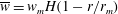
(1) A ‘top-hat’ plume with velocity profile
 $\overline{w}=w_{m}H(1-r/r_{m})$
where
$H$
is the Heaviside function, implying that
${\it\gamma}_{m}=1$
. In this case, both
${\rm\Delta}M>0$
and
${\rm\Delta}E>0$
due to the buoyancy. However, as
$(1-{\it\theta}_{m}/{\it\gamma}_{m})\mathit{Ri}=0$
, the plume does not entrain, i.e.
${\it\alpha}=0$
. The radius
$r_{m}$
will decrease in order to satisfy momentum and energy conservation, cf. (3.11).
$\overline{w}=w_{m}H(1-r/r_{m})$
where
$H$
is the Heaviside function, implying that
${\it\gamma}_{m}=1$
. In this case, both
${\rm\Delta}M>0$
and
${\rm\Delta}E>0$
due to the buoyancy. However, as
$(1-{\it\theta}_{m}/{\it\gamma}_{m})\mathit{Ri}=0$
, the plume does not entrain, i.e.
${\it\alpha}=0$
. The radius
$r_{m}$
will decrease in order to satisfy momentum and energy conservation, cf. (3.11). -
(2) A Gaussian plume with velocity profile
$\overline{w}=2w_{m}\exp (-2r^{2}/r_{m}^{2})$
, implying that
${\it\gamma}_{m}=4/3$
. Since
${\it\gamma}_{m}=4/3>1$
, the value of
${\rm\Delta}E/E$
is less negative for a Gaussian than for a top-hat plume. Consequently
$(1-{\it\theta}_{m}/{\it\gamma}_{m})\mathit{Ri}>0$
, implying that
${\it\alpha}>0$
: the Gaussian plume entrains in order to satisfy momentum and energy conservation. From (3.11) it follows that the solution is a column of fluid of constant radius.


In both cases considered here, the fluid accelerates as
 ${\rm\Delta}M>0$
while the radius is either narrowing (top-hat plume) or remains constant (Gaussian plume). Without turbulence production, i.e.
${\rm\Delta}M>0$
while the radius is either narrowing (top-hat plume) or remains constant (Gaussian plume). Without turbulence production, i.e.
 ${\it\delta}_{m}=0$
, a top-hat plume is not able to entrain. However, a Gaussian plume is able to entrain even in the absence of turbulence. Although a Gaussian profile clearly requires turbulence to maintain its shape, the argument above demonstrates that buoyancy provides plumes with an entrainment mechanism not directly associated with turbulence.
${\it\delta}_{m}=0$
, a top-hat plume is not able to entrain. However, a Gaussian plume is able to entrain even in the absence of turbulence. Although a Gaussian profile clearly requires turbulence to maintain its shape, the argument above demonstrates that buoyancy provides plumes with an entrainment mechanism not directly associated with turbulence.
5. Entrainment models
In this section, we look at the MTT and PB theories in the light of the Gaussian far-field entrainment relation
 ${\it\alpha}$
-MSG. While the MTT theory does not explicitly assume that profiles are Gaussian, it can nevertheless be cast into the form of
${\it\alpha}$
-MSG. While the MTT theory does not explicitly assume that profiles are Gaussian, it can nevertheless be cast into the form of
 ${\it\alpha}$
-MSG, as we will show. The PB theory assumes that
${\it\alpha}$
-MSG, as we will show. The PB theory assumes that
 ${\it\delta}_{m}$
takes a constant value
${\it\delta}_{m}$
takes a constant value
 ${\it\delta}_{\mathit{PB}}$
, while the MTT model assumes that the entrainment coefficient
${\it\delta}_{\mathit{PB}}$
, while the MTT model assumes that the entrainment coefficient
 ${\it\alpha}_{\mathit{MTT}}$
is a constant. These assumptions represent lines on the realisability surface of the entrainment relation, as shown in figure 1. It should be noted that the axes in this figure are not independent. Indeed, as argued in the previous section,
${\it\alpha}_{\mathit{MTT}}$
is a constant. These assumptions represent lines on the realisability surface of the entrainment relation, as shown in figure 1. It should be noted that the axes in this figure are not independent. Indeed, as argued in the previous section,
 ${\it\alpha}$
and
${\it\alpha}$
and
 ${\it\delta}_{m}$
are both expected to depend on
${\it\delta}_{m}$
are both expected to depend on
 $\mathit{Ri}$
and, if non-equilibrium effects are included, also on
$\mathit{Ri}$
and, if non-equilibrium effects are included, also on
 $z$
. In this light, the MTT and PB models form two limit cases: the MTT model assumes that
$z$
. In this light, the MTT and PB models form two limit cases: the MTT model assumes that
 ${\it\alpha}$
is independent of
${\it\alpha}$
is independent of
 $\mathit{Ri}$
, while the PB model assumes that
$\mathit{Ri}$
, while the PB model assumes that
 ${\it\delta}_{m}$
is independent of
${\it\delta}_{m}$
is independent of
 $\mathit{Ri}$
. Evidently, observations are required to determine under which circumstances the various models describe the physics accurately. We will examine the evidence for pure jets and plumes in an unstratified ambient in § 6.
$\mathit{Ri}$
. Evidently, observations are required to determine under which circumstances the various models describe the physics accurately. We will examine the evidence for pure jets and plumes in an unstratified ambient in § 6.
5.1. The PB entrainment model
Substitution of a constant value
 ${\it\delta}_{\mathit{PB}}$
into the entrainment relation (3.7) provides the following model for the entrainment coefficient:
${\it\delta}_{\mathit{PB}}$
into the entrainment relation (3.7) provides the following model for the entrainment coefficient:
 $$\begin{eqnarray}{\it\alpha}_{\mathit{PB}}(\mathit{Ri})=-{\textstyle \frac{3}{8}}{\it\delta}_{\mathit{PB}}+{\textstyle \frac{1}{4}}\mathit{Ri},\end{eqnarray}$$
or equivalently, in terms of the flux parameter
 ${\it\Gamma}$
(using
${\it\Gamma}$
(using
 ${\it\beta}_{g}=1$
, consistent with the
${\it\beta}_{g}=1$
, consistent with the
 ${\it\alpha}$
-MS relation),
${\it\alpha}$
-MS relation),
 $$\begin{eqnarray}{\it\alpha}_{\mathit{PB}}({\it\Gamma})=-{\textstyle \frac{3}{8}}{\it\delta}_{\mathit{PB}}+{\textstyle \frac{2}{5}}{\it\alpha}_{p}{\it\Gamma}.\end{eqnarray}$$
For a pure jet (
 ${\it\Gamma}=0$
) it follows that
${\it\Gamma}=0$
) it follows that
 ${\it\alpha}_{j}=-(3/8){\it\delta}_{\mathit{PB}}$
, implying that
${\it\alpha}_{j}=-(3/8){\it\delta}_{\mathit{PB}}$
, implying that
 ${\it\alpha}_{\mathit{PB}}={\it\alpha}_{j}+(2/5){\it\alpha}_{p}{\it\Gamma}$
. By substituting the pure plume condition
${\it\alpha}_{\mathit{PB}}={\it\alpha}_{j}+(2/5){\it\alpha}_{p}{\it\Gamma}$
. By substituting the pure plume condition
 ${\it\Gamma}=1$
(for which by definition
${\it\Gamma}=1$
(for which by definition
 ${\it\alpha}_{\mathit{PB}}={\it\alpha}_{p}$
) it follows directly that
${\it\alpha}_{\mathit{PB}}={\it\alpha}_{p}$
) it follows directly that
 $$\begin{eqnarray}{\it\alpha}_{p}={\textstyle \frac{5}{3}}{\it\alpha}_{j}.\end{eqnarray}$$
This remarkable prediction is mentioned in passing in List & Imberger (Reference List and Imberger1973, equation (25)) where an entrainment model is derived starting from straight-sidedness that is consistent with the entrainment model implied by the PB plume equations.
Here, we note that according to the PB model, the higher entrainment of the plume is a result not of buoyancy-enhanced turbulence production but of the entrainment associated with the mean flow. Substitution of (5.3) back into (5.2) results in the operational entrainment model (1.2). A striking feature of the PB model is that the solutions are straight-sided, as can be inferred from (3.12), which is a consequence of
 ${\it\delta}_{\mathit{PB}}$
being constant. Straight-sidedness is perhaps the most crucial assumption of the PB model and is a testable hypothesis. This is physically not realistic in the near field, where necking is often observed, and near the level of neutral buoyancy, where the plume spreads out. Indeed, in both cases one does not expect turbulence production to remain in proportion to
${\it\delta}_{\mathit{PB}}$
being constant. Straight-sidedness is perhaps the most crucial assumption of the PB model and is a testable hypothesis. This is physically not realistic in the near field, where necking is often observed, and near the level of neutral buoyancy, where the plume spreads out. Indeed, in both cases one does not expect turbulence production to remain in proportion to
 $w_{m}^{3}r_{m}$
.
$w_{m}^{3}r_{m}$
.
5.2. The MTT entrainment model
Substitution of a constant value
 ${\it\alpha}_{\mathit{MTT}}$
for
${\it\alpha}_{\mathit{MTT}}$
for
 ${\it\alpha}$
into the entrainment relation (3.7) results in
${\it\alpha}$
into the entrainment relation (3.7) results in
 $$\begin{eqnarray}{\it\delta}_{\mathit{MTT}}(\mathit{Ri})=-{\textstyle \frac{8}{3}}{\it\alpha}_{\mathit{MTT}}+{\textstyle \frac{2}{3}}\mathit{Ri}=-{\textstyle \frac{16}{15}}{\it\alpha}_{\mathit{MTT}}\left({\textstyle \frac{5}{2}}-{\it\Gamma}\right).\end{eqnarray}$$
It thus follows directly that the model predicts that pure plumes (
 ${\it\Gamma}=1$
) produce less turbulence than jets (
${\it\Gamma}=1$
) produce less turbulence than jets (
 ${\it\Gamma}=0$
). Moreover, according to the MTT entrainment model plumes are expected to be narrower than jets, since
${\it\Gamma}=0$
). Moreover, according to the MTT entrainment model plumes are expected to be narrower than jets, since
 $$\begin{eqnarray}\frac{\text{d}r_{m}}{\text{d}z}=2{\it\alpha}_{\mathit{MTT}}-\frac{1}{2}\mathit{Ri}=\frac{4{\it\alpha}_{\mathit{MTT}}}{5}\left(\frac{5}{2}-{\it\Gamma}\right).\end{eqnarray}$$
Equation (5.5), derived here via the entrainment relation, is consistent with van den Bremer & Hunt (Reference van den Bremer and Hunt2010, equation (2.14)). This prediction is contrary to observations, which typically indicate that plumes have a slightly greater spreading rate than jets (e.g. List Reference List1982). However, it should be noted that it is standard practice to choose a different value for
 ${\it\alpha}$
depending on whether one wishes to carry out jet or plume predictions, and the observed deficiency of the MTT entrainment model is therefore obscured. Nevertheless, for situations in which
${\it\alpha}$
depending on whether one wishes to carry out jet or plume predictions, and the observed deficiency of the MTT entrainment model is therefore obscured. Nevertheless, for situations in which
 $\mathit{Ri}$
varies as a function of
$\mathit{Ri}$
varies as a function of
 $z$
, e.g. for lazy/forced plumes in a neutral environment or plumes in stratified environments, one will have to decide on a single value for
$z$
, e.g. for lazy/forced plumes in a neutral environment or plumes in stratified environments, one will have to decide on a single value for
 ${\it\alpha}$
. The
${\it\alpha}$
. The
 $\mathit{Ri}$
dependence of the spreading rate in (5.5) is the reason why the MTT plume equations are able to predict plume necking in the near field for lazy plumes. Indeed, for
$\mathit{Ri}$
dependence of the spreading rate in (5.5) is the reason why the MTT plume equations are able to predict plume necking in the near field for lazy plumes. Indeed, for
 ${\it\Gamma}>5/2$
,
${\it\Gamma}>5/2$
,
 ${\it\delta}_{\mathit{MTT}}$
changes sign and
${\it\delta}_{\mathit{MTT}}$
changes sign and
 $\text{d}r_{m}/\text{d}z<0$
. Similarly, the model predicts the plume spreading out to infinity at the neutral buoyancy level. The capability to capture necking and spreading is an extremely useful feature of the MTT model, although further work is needed to understand the extent to which the model faithfully represents the underlying physical processes.
$\text{d}r_{m}/\text{d}z<0$
. Similarly, the model predicts the plume spreading out to infinity at the neutral buoyancy level. The capability to capture necking and spreading is an extremely useful feature of the MTT model, although further work is needed to understand the extent to which the model faithfully represents the underlying physical processes.
6. Pure jets and plumes in an unstratified environment
In this section we investigate entrainment for pure jets and plumes in an unstratified environment using data available in the literature. We focus on
 ${\it\alpha}$
,
${\it\alpha}$
,
 ${\it\delta}_{m}$
,
${\it\delta}_{m}$
,
 ${\it\gamma}_{m}$
and, in the case of a plume,
${\it\gamma}_{m}$
and, in the case of a plume,
 ${\it\theta}_{m}$
. Table 3 shows the values of these coefficients for the following studies: Papanicolaou & List (Reference Papanicolaou and List1988, PL88); Panchapakesan & Lumley (Reference Panchapakesan and Lumley1993a
, PL93); Shabbir & George (Reference Shabbir and George1994, SG94); Wang & Law (Reference Wang and Law2002, WL02); Craske (Reference Craske2015,
${\it\theta}_{m}$
. Table 3 shows the values of these coefficients for the following studies: Papanicolaou & List (Reference Papanicolaou and List1988, PL88); Panchapakesan & Lumley (Reference Panchapakesan and Lumley1993a
, PL93); Shabbir & George (Reference Shabbir and George1994, SG94); Wang & Law (Reference Wang and Law2002, WL02); Craske (Reference Craske2015,
 $\mathit{Re}=1600$
, CvR15c); Craske & van Reeuwijk (Reference Craske and van Reeuwijk2015a
,
$\mathit{Re}=1600$
, CvR15c); Craske & van Reeuwijk (Reference Craske and van Reeuwijk2015a
,
 $\mathit{Re}=4815$
, CvR15a) and Ezzamel et al. (Reference Ezzamel, Salizzoni and Hunt2015, ESH15). Often, there is more than one way in which a coefficient can be inferred from a given data set, resulting in some systematic uncertainty in the estimates. For example, to estimate
$\mathit{Re}=4815$
, CvR15a) and Ezzamel et al. (Reference Ezzamel, Salizzoni and Hunt2015, ESH15). Often, there is more than one way in which a coefficient can be inferred from a given data set, resulting in some systematic uncertainty in the estimates. For example, to estimate
 ${\it\alpha}$
from the direct numerical simulation data, Craske & van Reeuwijk (Reference Craske and van Reeuwijk2015a
) compute
${\it\alpha}$
from the direct numerical simulation data, Craske & van Reeuwijk (Reference Craske and van Reeuwijk2015a
) compute
 $(\text{d}Q/\text{d}z)/(2M^{1/2})$
directly, whereas experimentalists (see, e.g., Wang & Law Reference Wang and Law2002) typically prefer to infer
$(\text{d}Q/\text{d}z)/(2M^{1/2})$
directly, whereas experimentalists (see, e.g., Wang & Law Reference Wang and Law2002) typically prefer to infer
 ${\it\alpha}$
from the spreading rate of the plume by fitting a Gaussian curve to the profiles of mean velocity. Only in the case of fully self-similar Gaussian plumes are these two approaches equivalent. The cases selected were chosen because they provide the value of
${\it\alpha}$
from the spreading rate of the plume by fitting a Gaussian curve to the profiles of mean velocity. Only in the case of fully self-similar Gaussian plumes are these two approaches equivalent. The cases selected were chosen because they provide the value of
 ${\it\alpha}$
, the profiles of mean velocity, Reynolds stress and, in the case of a plume, mean buoyancy. This provides sufficient information to evaluate all terms in the entrainment relation
${\it\alpha}$
, the profiles of mean velocity, Reynolds stress and, in the case of a plume, mean buoyancy. This provides sufficient information to evaluate all terms in the entrainment relation
 ${\it\alpha}$
-MS, (3.6). The standard procedure was to digitise the profiles and then to evaluate the coefficients numerically, converting to the scales used in this paper where required. Where possible, we made use of function fits of the data (WL02). The profile coefficients stated for ESH15 were calculated directly from the far-field source data and the values of
${\it\alpha}$
-MS, (3.6). The standard procedure was to digitise the profiles and then to evaluate the coefficients numerically, converting to the scales used in this paper where required. Where possible, we made use of function fits of the data (WL02). The profile coefficients stated for ESH15 were calculated directly from the far-field source data and the values of
 ${\it\alpha}$
were determined directly from the spreading rate
${\it\alpha}$
were determined directly from the spreading rate
 $\text{d}r_{m}/\text{d}z$
(P. Salizzoni, private communication). It should be noted that the values of
$\text{d}r_{m}/\text{d}z$
(P. Salizzoni, private communication). It should be noted that the values of
 ${\it\alpha}$
for the ESH15 dataset presented here are significantly larger than those presented in Ezzamel et al. (Reference Ezzamel, Salizzoni and Hunt2015), which were estimated from the continuity equation. The underprediction is due to a systematic error associated with a small but significant co-flow (P. Salizzoni, private communication). The last four rows of table 3 (highlighted
${\it\alpha}$
for the ESH15 dataset presented here are significantly larger than those presented in Ezzamel et al. (Reference Ezzamel, Salizzoni and Hunt2015), which were estimated from the continuity equation. The underprediction is due to a systematic error associated with a small but significant co-flow (P. Salizzoni, private communication). The last four rows of table 3 (highlighted
 $^{a}$
) contain the converted Kaminski coefficients
$^{a}$
) contain the converted Kaminski coefficients
 $A$
and
$A$
and
 $C$
(see appendix A). Here, we note that our estimate for
$C$
(see appendix A). Here, we note that our estimate for
 ${\it\delta}_{m}$
in WL02 is lower than for WL02
${\it\delta}_{m}$
in WL02 is lower than for WL02
 $^{a}$
. Having determined
$^{a}$
. Having determined
 ${\it\delta}_{m}$
,
${\it\delta}_{m}$
,
 ${\it\gamma}_{m}$
and
${\it\gamma}_{m}$
and
 ${\it\theta}_{m}$
, the indirect estimate
${\it\theta}_{m}$
, the indirect estimate
 ${\it\alpha}$
-MS can be determined and compared with the direct estimate
${\it\alpha}$
-MS can be determined and compared with the direct estimate
 ${\it\alpha}$
. We will first show that
${\it\alpha}$
. We will first show that
 ${\it\alpha}$
-MS provides a reasonably complete description of the entrainment physics and then investigate the contributions of the individual terms comprising
${\it\alpha}$
-MS provides a reasonably complete description of the entrainment physics and then investigate the contributions of the individual terms comprising
 ${\it\alpha}$
-MS.
${\it\alpha}$
-MS.
Table 3. The observed entrainment coefficient and profile coefficients in jets and plumes. The data sources are Papanicolaou & List (Reference Papanicolaou and List1988, PL88); Panchapakesan & Lumley (Reference Panchapakesan and Lumley1993a ,Reference Panchapakesan and Lumley b , PL93a, PL93b); Shabbir & George (Reference Shabbir and George1994, SG94); Wang & Law (Reference Wang and Law2002, WL02); Craske (Reference Craske2015, CvR15c); Craske & van Reeuwijk (Reference Craske and van Reeuwijk2015a , CvR15a) and Ezzamel et al. (Reference Ezzamel, Salizzoni and Hunt2015, ESH15).

a Data converted from Kaminski et al. (Reference Kaminski, Tait and Carazzo2005), Carazzo et al. (Reference Carazzo, Kaminski and Tait2006) using appendix A.
b
Here,
 ${\it\Gamma}=0.5$
is assumed as a first-order approximation, because, as Carazzo et al. (Reference Carazzo, Kaminski and Tait2006) point out, the data from Panchapakesan & Lumley (Reference Panchapakesan and Lumley1993b
, PL93b) pertain to an intermediate distance from a forced release, and therefore
${\it\Gamma}=0.5$
is assumed as a first-order approximation, because, as Carazzo et al. (Reference Carazzo, Kaminski and Tait2006) point out, the data from Panchapakesan & Lumley (Reference Panchapakesan and Lumley1993b
, PL93b) pertain to an intermediate distance from a forced release, and therefore
 $0<{\it\Gamma}<1$
.
$0<{\it\Gamma}<1$
.
The last column in table 3 presents the absolute relative difference between the observed value of
 ${\it\alpha}$
and the estimate
${\it\alpha}$
and the estimate
 ${\it\alpha}$
-MS. The two estimates generally agree to within 5 % for the jet data, and to within 15 % for the plume data. The ESH15 data have larger error bars, which are probably due to the large scatter in the Reynolds-stress profiles and the large value of
${\it\alpha}$
-MS. The two estimates generally agree to within 5 % for the jet data, and to within 15 % for the plume data. The ESH15 data have larger error bars, which are probably due to the large scatter in the Reynolds-stress profiles and the large value of
 ${\it\theta}_{m}$
. Even though the entrainment relation
${\it\theta}_{m}$
. Even though the entrainment relation
 ${\it\alpha}$
-MS does not take into account contributions due to turbulence and pressure, the generally close agreement of the two estimates of
${\it\alpha}$
-MS does not take into account contributions due to turbulence and pressure, the generally close agreement of the two estimates of
 ${\it\alpha}$
confirms that
${\it\alpha}$
confirms that
 ${\it\alpha}$
-MS captures the primary entrainment mechanisms. Pressure redistribution and longitudinal turbulence production are responsible for the larger absolute relative difference between the two estimates of
${\it\alpha}$
-MS captures the primary entrainment mechanisms. Pressure redistribution and longitudinal turbulence production are responsible for the larger absolute relative difference between the two estimates of
 ${\it\alpha}$
for plumes than for jets, as can be inferred from direct numerical simulation data: the plume simulations of CvR15c indicate that
${\it\alpha}$
for plumes than for jets, as can be inferred from direct numerical simulation data: the plume simulations of CvR15c indicate that
 ${\it\delta}_{g}=-0.20>-0.23={\it\delta}_{m}$
due to contributions from
${\it\delta}_{g}=-0.20>-0.23={\it\delta}_{m}$
due to contributions from
 ${\it\delta}_{f}$
and
${\it\delta}_{f}$
and
 ${\it\delta}_{p}$
, and with these contributions included the difference between the two estimates is less than 5 %.
${\it\delta}_{p}$
, and with these contributions included the difference between the two estimates is less than 5 %.
A striking feature of the data in table 3 is that the value of
 ${\it\delta}_{m}$
is very similar for the jet and plume data, indicating that turbulence production is quite insensitive to
${\it\delta}_{m}$
is very similar for the jet and plume data, indicating that turbulence production is quite insensitive to
 $\mathit{Ri}$
. This in turn suggests that the PB entrainment model may appropriately capture the dynamics of jets and plumes in an unstratified environment when
$\mathit{Ri}$
. This in turn suggests that the PB entrainment model may appropriately capture the dynamics of jets and plumes in an unstratified environment when
 $0\leqslant {\it\Gamma}\leqslant 1$
. This hypothesis is further explored in figure 2, where the decomposed contributions to
$0\leqslant {\it\Gamma}\leqslant 1$
. This hypothesis is further explored in figure 2, where the decomposed contributions to
 ${\it\alpha}$
-MS of table 3 are presented graphically, together with the direct estimation of
${\it\alpha}$
-MS of table 3 are presented graphically, together with the direct estimation of
 ${\it\alpha}$
(squares). The dashed lines represent the averages of
${\it\alpha}$
(squares). The dashed lines represent the averages of
 $-\langle {\it\delta}_{m}/(2{\it\gamma}_{m})\rangle$
and
$-\langle {\it\delta}_{m}/(2{\it\gamma}_{m})\rangle$
and
 $\langle {\it\alpha}\text{-}\text{MS}\rangle$
, where the operator
$\langle {\it\alpha}\text{-}\text{MS}\rangle$
, where the operator
 $\langle \cdot \rangle$
denotes the average over the jet/plume data. It should be noted that the WL02
$\langle \cdot \rangle$
denotes the average over the jet/plume data. It should be noted that the WL02
 $^{a}$
data were not included in the average to avoid double counting. Figure 2 reinforces the fact that
$^{a}$
data were not included in the average to avoid double counting. Figure 2 reinforces the fact that
 $-{\it\delta}_{m}/(2{\it\gamma}_{m})$
is similar for a pure jet and a pure plume. Furthermore, for a pure plume the ratio of the average value of
$-{\it\delta}_{m}/(2{\it\gamma}_{m})$
is similar for a pure jet and a pure plume. Furthermore, for a pure plume the ratio of the average value of
 $\langle {\it\alpha}\text{-}\text{MS}\rangle$
to
$\langle {\it\alpha}\text{-}\text{MS}\rangle$
to
 $-\langle {\it\delta}_{m}/(2{\it\gamma}_{m})\rangle$
is within 5 % of the value of
$-\langle {\it\delta}_{m}/(2{\it\gamma}_{m})\rangle$
is within 5 % of the value of
 $5/3$
predicted by the PB entrainment model.
$5/3$
predicted by the PB entrainment model.

Figure 2. Individual terms of the entrainment relation
 ${\it\alpha}$
-MS compared with a direct estimate of
${\it\alpha}$
-MS compared with a direct estimate of
 ${\it\alpha}$
(squares). The dashed lines are the averages of the individual terms of
${\it\alpha}$
(squares). The dashed lines are the averages of the individual terms of
 ${\it\alpha}$
-MS, (3.6).
${\it\alpha}$
-MS, (3.6).
An interesting implication of the fact that
 ${\it\delta}_{m}$
remains approximately constant is that the often-used argument (List Reference List1982; Carazzo et al.
Reference Carazzo, Kaminski and Tait2006) of buoyancy-enhanced turbulence being the primary mechanism for the higher entrainment coefficient of plumes is not supported by the data. Indeed, enhanced turbulence levels would be expected to result in a larger value for
${\it\delta}_{m}$
remains approximately constant is that the often-used argument (List Reference List1982; Carazzo et al.
Reference Carazzo, Kaminski and Tait2006) of buoyancy-enhanced turbulence being the primary mechanism for the higher entrainment coefficient of plumes is not supported by the data. Indeed, enhanced turbulence levels would be expected to result in a larger value for
 ${\it\delta}_{m}$
. Instead, it is a mean contribution to entrainment associated with the
${\it\delta}_{m}$
. Instead, it is a mean contribution to entrainment associated with the
 $\mathit{Ri}$
dependence that is responsible for the higher entrainment coefficient.
$\mathit{Ri}$
dependence that is responsible for the higher entrainment coefficient.
List & Imberger (Reference List and Imberger1973) and List (Reference List1982) observed that plumes and jets spread at a very similar rate, which, via (3.12), provides support for
 ${\it\delta}_{m}$
remaining approximately constant. Kaminski et al. (Reference Kaminski, Tait and Carazzo2005) calculate
${\it\delta}_{m}$
remaining approximately constant. Kaminski et al. (Reference Kaminski, Tait and Carazzo2005) calculate
 ${\it\delta}_{m}$
(which is proportional to their
${\it\delta}_{m}$
(which is proportional to their
 $C$
parameter, see appendix A) for pure plumes and then use the entrainment relation
$C$
parameter, see appendix A) for pure plumes and then use the entrainment relation
 ${\it\alpha}$
-MS to observe that this value is in close agreement with the jet data, and in accordance with previous observations that the Reynolds-stress profiles in jets and plumes are very similar (Panchapakesan & Lumley Reference Panchapakesan and Lumley1993a
; Wang & Law Reference Wang and Law2002). Lastly, the forced plume experiments of Wang & Law (Reference Wang and Law2002), Matulka et al. (Reference Matulka, Lopez, Redondo and Tarquis2014) and Ezzamel et al. (Reference Ezzamel, Salizzoni and Hunt2015) show that the measured entrainment coefficient is in good agreement with the PB model.
${\it\alpha}$
-MS to observe that this value is in close agreement with the jet data, and in accordance with previous observations that the Reynolds-stress profiles in jets and plumes are very similar (Panchapakesan & Lumley Reference Panchapakesan and Lumley1993a
; Wang & Law Reference Wang and Law2002). Lastly, the forced plume experiments of Wang & Law (Reference Wang and Law2002), Matulka et al. (Reference Matulka, Lopez, Redondo and Tarquis2014) and Ezzamel et al. (Reference Ezzamel, Salizzoni and Hunt2015) show that the measured entrainment coefficient is in good agreement with the PB model.
In spite of the agreement that entrainment in forced plumes has with the PB model, the question of the most suitable parameterisation of entrainment in lazy plumes (
 ${\it\Gamma}>1$
) remains open. Bhat & Narasimha (Reference Bhat and Narasimha1996) report an observed narrowing in a heated (and consequently lazy) plume, which is broadly consistent with the MTT model for entrainment. However, in the absence of more comprehensive experimental and numerical data one is forced to accept the possibility that the true behaviour of the entrainment coefficient in lazy plumes might not coincide with either of the idealised models of PB and MTT. For lazy plumes one therefore assumes that
${\it\Gamma}>1$
) remains open. Bhat & Narasimha (Reference Bhat and Narasimha1996) report an observed narrowing in a heated (and consequently lazy) plume, which is broadly consistent with the MTT model for entrainment. However, in the absence of more comprehensive experimental and numerical data one is forced to accept the possibility that the true behaviour of the entrainment coefficient in lazy plumes might not coincide with either of the idealised models of PB and MTT. For lazy plumes one therefore assumes that
 ${\it\alpha}$
traces a more complicated curve on the realisability surface of the entrainment relation illustrated in figure 1.
${\it\alpha}$
traces a more complicated curve on the realisability surface of the entrainment relation illustrated in figure 1.
7. Entrainment at constant
$\mathit{Ri}$

Further understanding of the way in which
 ${\it\alpha}$
depends on
${\it\alpha}$
depends on
 $\mathit{Ri}$
requires knowledge of the dependence of
$\mathit{Ri}$
requires knowledge of the dependence of
 ${\it\delta}_{g},{\it\gamma}_{g}$
and
${\it\delta}_{g},{\it\gamma}_{g}$
and
 ${\it\theta}_{g}$
on
${\it\theta}_{g}$
on
 $\mathit{Ri}$
. Unfortunately, controlled observation of situations in which
$\mathit{Ri}$
. Unfortunately, controlled observation of situations in which
 $\mathit{Ri}$
is constant is difficult because (i), with the exception of pure jets and plumes,
$\mathit{Ri}$
is constant is difficult because (i), with the exception of pure jets and plumes,
 $\mathit{Ri}$
typically varies in
$\mathit{Ri}$
typically varies in
 $z$
and (ii) changes in
$z$
and (ii) changes in
 $\mathit{Ri}$
are often accompanied by additional effects, such as the near-field development of a plume. To investigate the dependence of entrainment on
$\mathit{Ri}$
are often accompanied by additional effects, such as the near-field development of a plume. To investigate the dependence of entrainment on
 $\mathit{Ri}$
in isolation one would ideally conduct an experiment or simulation on a plume in which
$\mathit{Ri}$
in isolation one would ideally conduct an experiment or simulation on a plume in which
 $\mathit{Ri}$
remains constant. In this section we therefore present solutions, based on those originally obtained by Batchelor (Reference Batchelor1954) and Caulfield & Woods (Reference Caulfield and Woods1998), for cases in which
$\mathit{Ri}$
remains constant. In this section we therefore present solutions, based on those originally obtained by Batchelor (Reference Batchelor1954) and Caulfield & Woods (Reference Caulfield and Woods1998), for cases in which
 $$\begin{eqnarray}{\displaystyle \frac{\text{d}\mathit{Ri}}{\text{d}z}}=0,\end{eqnarray}$$
before discussing the ways in which (7.1) might be realised in practice. Substitution for
 $\mathit{Ri}$
in (2.8) and (2.10) gives
$\mathit{Ri}$
in (2.8) and (2.10) gives
 $$\begin{eqnarray}\displaystyle & \displaystyle {\displaystyle \frac{\text{d}}{\text{d}z}}({\it\beta}_{g}M)=\frac{M^{3/2}}{Q}\mathit{Ri}, & \displaystyle\end{eqnarray}$$
 $$\begin{eqnarray}\displaystyle & \displaystyle {\displaystyle \frac{\text{d}}{\text{d}z}}\left({\it\gamma}_{g}\frac{M^{2}}{Q}\right)=({\it\delta}_{g}+2{\it\theta}_{m}\mathit{Ri})\frac{M^{5/2}}{Q^{2}}, & \displaystyle\end{eqnarray}$$
 $\mathit{Ri}$
in terms of
$\mathit{Ri}$
in terms of
 $Q,M$
and
$Q,M$
and
 $F$
using (2.16), (7.1) implies that
$F$
using (2.16), (7.1) implies that  $$\begin{eqnarray}{\displaystyle \frac{\text{d}F}{\text{d}z}}={\it\theta}_{m}\mathit{Ri}{\displaystyle \frac{\text{d}}{\text{d}z}}\left(\frac{M^{5/2}}{Q^{2}}\right).\end{eqnarray}$$
It should be noted that although we have not yet invoked an equation for buoyancy transport, (7.4) is a consistency requirement that determines the behaviour of
 $F$
for a given
$F$
for a given
 $\mathit{Ri}$
. We address the physical means of ensuring that
$\mathit{Ri}$
. We address the physical means of ensuring that
 $F$
behaves in this way in the following paragraph. Seeking solutions
$F$
behaves in this way in the following paragraph. Seeking solutions
 $$\begin{eqnarray}Q=Q_{0}\left(\frac{z}{z_{0}}\right)^{q},\quad M=M_{0}\left(\frac{z}{z_{0}}\right)^{m},\quad F=F_{0}\left(\frac{z}{z_{0}}\right)^{f},\end{eqnarray}$$
one finds
 $$\begin{eqnarray}q=3+\frac{a}{2},\quad m=4+a,\quad f=4+\frac{3a}{2},\end{eqnarray}$$
where, making use of
 ${\it\alpha}$
-S to eliminate
${\it\alpha}$
-S to eliminate
 ${\it\delta}_{g}$
and
${\it\delta}_{g}$
and
 ${\it\gamma}_{g}$
,
${\it\gamma}_{g}$
,
 $$\begin{eqnarray}a\equiv \frac{6\mathit{Ri}/{\it\beta}_{g}-16{\it\alpha}}{4{\it\alpha}-\mathit{Ri}/{\it\beta}_{g}}.\end{eqnarray}$$
When
 $\mathit{Ri}=8{\it\alpha}_{p}{\it\beta}_{g}/5$
,
$\mathit{Ri}=8{\it\alpha}_{p}{\it\beta}_{g}/5$
,
 $a=-8/3$
and
$a=-8/3$
and
 $q=5/3,m=4/3,f=0$
, which is consistent with the classical self-similar plume solutions. Furthermore,
$q=5/3,m=4/3,f=0$
, which is consistent with the classical self-similar plume solutions. Furthermore,
 $$\begin{eqnarray}Q_{0}=\left(\frac{z_{0}^{5}F_{0}\mathit{Ri}^{4}}{{\it\beta}_{g}^{5}{\it\theta}_{m}(a+4)^{5}}\right)^{1/3},\quad M_{0}=\left(\frac{z_{0}^{2}F_{0}\mathit{Ri}}{{\it\beta}_{g}^{2}{\it\theta}_{m}(a+4)^{2}}\right)^{2/3}\end{eqnarray}$$
for prescribed values of
 $\mathit{Ri}$
and
$\mathit{Ri}$
and
 $F_{0}$
. The classical jet solutions correspond to the limit
$F_{0}$
. The classical jet solutions correspond to the limit
 $a\rightarrow -4,F_{0}\rightarrow 0,\mathit{Ri}\rightarrow 0$
, in such a way that
$a\rightarrow -4,F_{0}\rightarrow 0,\mathit{Ri}\rightarrow 0$
, in such a way that
 $Q_{0}$
and
$Q_{0}$
and
 $M_{0}$
remain
$M_{0}$
remain
 $O(1)$
. Since
$O(1)$
. Since
 $\mathit{Ri}$
is constant, a notable feature of these solutions is that the spreading rate of the plume is a constant that depends on
$\mathit{Ri}$
is constant, a notable feature of these solutions is that the spreading rate of the plume is a constant that depends on
 $\mathit{Ri}$
and the profile coefficients. Observations of
$\mathit{Ri}$
and the profile coefficients. Observations of
 $\text{d}r_{m}/\text{d}z$
for a given
$\text{d}r_{m}/\text{d}z$
for a given
 $\mathit{Ri}$
therefore provide a convenient way of establishing the relationship between the profile coefficients and
$\mathit{Ri}$
therefore provide a convenient way of establishing the relationship between the profile coefficients and
 $\mathit{Ri}$
without direct measurement. Specifically, if a spreading rate
$\mathit{Ri}$
without direct measurement. Specifically, if a spreading rate
 $\text{d}r_{m}/\text{d}z$
is observed, one can use the implicit relation (see table 2)
$\text{d}r_{m}/\text{d}z$
is observed, one can use the implicit relation (see table 2)
 $$\begin{eqnarray}{\displaystyle \frac{\text{d}r_{m}}{\text{d}z}}(\mathit{Ri})=-\frac{{\it\delta}_{g}(\mathit{Ri})}{{\it\gamma}_{g}(\mathit{Ri})}+\frac{3}{2}\left(\frac{1}{{\it\beta}_{g}(\mathit{Ri})}-\frac{4}{3}\frac{{\it\theta}_{m}(\mathit{Ri})}{{\it\gamma}_{g}(\mathit{Ri})}\right)\mathit{Ri}\end{eqnarray}$$
to deduce the possible dependence of the profile coefficients on
 $\mathit{Ri}$
. If, in addition, the volume flux is measured, then one can couple (7.9) with the relation for
$\mathit{Ri}$
. If, in addition, the volume flux is measured, then one can couple (7.9) with the relation for
 ${\it\alpha}$
to further restrict the possible form of dependence on
${\it\alpha}$
to further restrict the possible form of dependence on
 $\mathit{Ri}$
that the profile coefficients might have. In this way it is possible to deduce higher-order aspects of the flow by measuring lower-order bulk quantities.
$\mathit{Ri}$
that the profile coefficients might have. In this way it is possible to deduce higher-order aspects of the flow by measuring lower-order bulk quantities.
From a practical perspective it is necessary to consider how a constant-
 $\mathit{Ri}$
flow could be realised in the laboratory or in a numerical simulation. To this end, we assume that the buoyancy flux in the plume can be modified either directly via a heat source
$\mathit{Ri}$
flow could be realised in the laboratory or in a numerical simulation. To this end, we assume that the buoyancy flux in the plume can be modified either directly via a heat source
 $S(z)$
or indirectly via a stratified environment with buoyancy frequency
$S(z)$
or indirectly via a stratified environment with buoyancy frequency
 $N(z)$
. With a heat source included, the conservation equation for the buoyancy flux becomes (cf. (2.9))
$N(z)$
. With a heat source included, the conservation equation for the buoyancy flux becomes (cf. (2.9))
 $$\begin{eqnarray}{\displaystyle \frac{\text{d}F}{\text{d}z}}=\frac{fF_{0}}{z}\left(\frac{z}{z_{0}}\right)^{f}=-\frac{{\it\theta}_{m}}{{\it\theta}_{g}}N^{2}Q+S,\quad \text{where}~N^{2}\equiv N_{0}^{2}\left(\frac{z}{z_{0}}\right)^{a}.\end{eqnarray}$$
When
 $N=0$
(an unstratified environment), the power-law behaviour can be obtained by using a buoyancy source
$N=0$
(an unstratified environment), the power-law behaviour can be obtained by using a buoyancy source
 $S=fF/z$
, where
$S=fF/z$
, where
 $F$
(see (7.5)) and
$F$
(see (7.5)) and
 $f$
(see (7.6)) are known functions of
$f$
(see (7.6)) are known functions of
 $\mathit{Ri}$
, the special case of constant
$\mathit{Ri}$
, the special case of constant
 $S$
having been examined by Hunt & Kaye (Reference Hunt and Kaye2005). In a numerical simulation, a source of buoyancy of this kind can be imposed locally by forcing the buoyancy
$S$
having been examined by Hunt & Kaye (Reference Hunt and Kaye2005). In a numerical simulation, a source of buoyancy of this kind can be imposed locally by forcing the buoyancy
 $b$
by an amount
$b$
by an amount
 $f\overline{w}\overline{b}/z$
. Experimentally, this could be realised by making the plume fluid conductive and subjecting it to a potential difference (see Bhat & Narasimha Reference Bhat and Narasimha1996; Agrawal & Prasad Reference Agrawal and Prasad2004). However, great care would be required to ensure that the radial dependence of the forcing function was fully understood, as it would most likely influence parameters such as
$f\overline{w}\overline{b}/z$
. Experimentally, this could be realised by making the plume fluid conductive and subjecting it to a potential difference (see Bhat & Narasimha Reference Bhat and Narasimha1996; Agrawal & Prasad Reference Agrawal and Prasad2004). However, great care would be required to ensure that the radial dependence of the forcing function was fully understood, as it would most likely influence parameters such as
 ${\it\delta}_{g}$
and
${\it\delta}_{g}$
and
 ${\it\theta}_{g}$
.
${\it\theta}_{g}$
.
Alternatively, a forcing in the buoyancy equation can be achieved by imposing a stratification in the ambient (
 $N^{2}\neq 0$
), resulting in
$N^{2}\neq 0$
), resulting in
 $$\begin{eqnarray}Q_{0}=-\text{i}\left(\frac{N_{0}^{2}}{fm{\it\theta}_{g}{\it\beta}_{g}}\right)^{1/2}\frac{4{\it\alpha}^{2}z_{0}^{3}}{q^{2}},\quad M_{0}=-\frac{4{\it\alpha}^{2}N_{0}^{2}z_{0}^{4}}{fmq^{2}{\it\theta}_{g}{\it\beta}_{g}},\quad F_{0}=-\frac{{\it\theta}_{m}}{{\it\theta}_{g}}\frac{N_{0}^{2}z_{0}}{f}Q_{0}.\end{eqnarray}$$
The condition that
 $Q_{0}$
and
$Q_{0}$
and
 $F_{0}$
must remain real-valued can be satisfied in two ways: (1)
$F_{0}$
must remain real-valued can be satisfied in two ways: (1)
 $N_{0}^{2}<0$
and
$N_{0}^{2}<0$
and
 $f>0$
, implying that
$f>0$
, implying that
 $a>-8/3$
, i.e. an increasing buoyancy flux in an unstable stratification (Batchelor Reference Batchelor1954); or (2)
$a>-8/3$
, i.e. an increasing buoyancy flux in an unstable stratification (Batchelor Reference Batchelor1954); or (2)
 $N_{0}^{2}>0$
and
$N_{0}^{2}>0$
and
 $f<0$
, implying that
$f<0$
, implying that
 $-4<a<-8/3$
, i.e. a decreasing buoyancy flux in a stable stratification (Caulfield & Woods Reference Caulfield and Woods1998). While it is typically assumed that
$-4<a<-8/3$
, i.e. a decreasing buoyancy flux in a stable stratification (Caulfield & Woods Reference Caulfield and Woods1998). While it is typically assumed that
 ${\it\alpha}$
is constant in these solutions, here
${\it\alpha}$
is constant in these solutions, here
 ${\it\alpha}$
depends on
${\it\alpha}$
depends on
 $\mathit{Ri}$
and therefore on
$\mathit{Ri}$
and therefore on
 $a$
:
$a$
:
 $$\begin{eqnarray}{\it\alpha}=-\frac{{\it\delta}_{g}}{2{\it\gamma}_{g}}\left(4\left(\frac{a+4}{a+6}\right)\left(\frac{{\it\theta}_{m}}{{\it\gamma}_{g}{\it\beta}_{g}}-1\right)+1\right)^{-1}.\end{eqnarray}$$
Equation (7.12) therefore relates the scaling associated with an ambient stratification to the entrainment coefficient, subject to knowledge of the profile coefficients. When
 $a>-8/3$
, the exponent
$a>-8/3$
, the exponent
 $f>0$
, implying that the buoyancy flux increases with height. The plumes that these solutions describe develop in the absence of a heat source and were first identified by Batchelor (Reference Batchelor1954). They are lazy plumes because
$f>0$
, implying that the buoyancy flux increases with height. The plumes that these solutions describe develop in the absence of a heat source and were first identified by Batchelor (Reference Batchelor1954). They are lazy plumes because
 $a>-8/3$
implies that
$a>-8/3$
implies that
 ${\it\Gamma}>1$
. However, it is clear that the unstable stratification required for this regime would be difficult to realise in practice and that the methods of heating the plume described above provide a more practical means of investigating lazy plumes. Indeed, the use of a stratification is best suited to the investigation of forced plumes, which are obtained over the interval
${\it\Gamma}>1$
. However, it is clear that the unstable stratification required for this regime would be difficult to realise in practice and that the methods of heating the plume described above provide a more practical means of investigating lazy plumes. Indeed, the use of a stratification is best suited to the investigation of forced plumes, which are obtained over the interval
 $-4<a<-8/3$
, for which
$-4<a<-8/3$
, for which
 $f<0$
and
$f<0$
and
 $0<{\it\Gamma}<1$
. These solutions correspond to a stratification that decays rapidly enough to maintain positive buoyancy flux in the plume, in spite of the fact that
$0<{\it\Gamma}<1$
. These solutions correspond to a stratification that decays rapidly enough to maintain positive buoyancy flux in the plume, in spite of the fact that
 $f<0$
(Caulfield & Woods Reference Caulfield and Woods1998). Pure plume and jet solutions correspond to limits
$f<0$
(Caulfield & Woods Reference Caulfield and Woods1998). Pure plume and jet solutions correspond to limits
 $f\rightarrow 0,z_{0}\rightarrow 0$
with
$f\rightarrow 0,z_{0}\rightarrow 0$
with
 $f^{3/8}/z_{0}=O(1)$
and
$f^{3/8}/z_{0}=O(1)$
and
 $m\rightarrow 0,z_{0}\rightarrow 0$
with
$m\rightarrow 0,z_{0}\rightarrow 0$
with
 $m^{1/4}/z_{0}=O(1)$
respectively (see Caulfield & Woods Reference Caulfield and Woods1998, for further details).
$m^{1/4}/z_{0}=O(1)$
respectively (see Caulfield & Woods Reference Caulfield and Woods1998, for further details).
Constant
 $\mathit{Ri}$
similarity solutions provide a useful means of investigating entrainment in plumes because they are not restricted to the near field. Moreover, the freedom to modify
$\mathit{Ri}$
similarity solutions provide a useful means of investigating entrainment in plumes because they are not restricted to the near field. Moreover, the freedom to modify
 $\mathit{Ri}$
via an ambient stratification or a direct source of heating, or both, is valuable, because the resulting profile coefficients may well depend on the particular method employed.
$\mathit{Ri}$
via an ambient stratification or a direct source of heating, or both, is valuable, because the resulting profile coefficients may well depend on the particular method employed.
8. Concluding remarks
This paper focused on the restrictions imposed upon the entrainment coefficient
 ${\it\alpha}$
by the conservation equation of mean kinetic energy. By integrating the Reynolds-averaged axisymmetric conservation equation for volume, streamwise momentum, buoyancy and mean kinetic energy over the radius
${\it\alpha}$
by the conservation equation of mean kinetic energy. By integrating the Reynolds-averaged axisymmetric conservation equation for volume, streamwise momentum, buoyancy and mean kinetic energy over the radius
 $r$
, four coupled ODEs were obtained with three independent variables,
$r$
, four coupled ODEs were obtained with three independent variables,
 $Q$
,
$Q$
,
 $M$
and
$M$
and
 $F$
. From the requirement that all four equations must be satisfied simultaneously, a restriction on the entrainment coefficient
$F$
. From the requirement that all four equations must be satisfied simultaneously, a restriction on the entrainment coefficient
 ${\it\alpha}$
was obtained, which was referred to as an entrainment relation. The entrainment relation decomposes
${\it\alpha}$
was obtained, which was referred to as an entrainment relation. The entrainment relation decomposes
 ${\it\alpha}$
into contributions due to turbulence production, buoyancy and changes in the profile coefficients. Entrainment due to buoyancy is primarily associated with mean-flow entrainment, i.e. turbulence does not play a direct role. As the normalised momentum- and energy-flux divergences contribute oppositely to entrainment, the shapes of the velocity and buoyancy profiles are a crucial factor in determining the net effect of buoyancy. The entrainment relation generalises previous entrainment relations that only incorporated mean-flow components (Kaminski et al.
Reference Kaminski, Tait and Carazzo2005) and fully self-similar mean profiles (Fox Reference Fox1970). The resulting hierarchy of entrainment relations is summarised in table 1.
${\it\alpha}$
into contributions due to turbulence production, buoyancy and changes in the profile coefficients. Entrainment due to buoyancy is primarily associated with mean-flow entrainment, i.e. turbulence does not play a direct role. As the normalised momentum- and energy-flux divergences contribute oppositely to entrainment, the shapes of the velocity and buoyancy profiles are a crucial factor in determining the net effect of buoyancy. The entrainment relation generalises previous entrainment relations that only incorporated mean-flow components (Kaminski et al.
Reference Kaminski, Tait and Carazzo2005) and fully self-similar mean profiles (Fox Reference Fox1970). The resulting hierarchy of entrainment relations is summarised in table 1.
The entrainment relation, which is a physical constraint upon
 ${\it\alpha}$
, must be considered separately from an entrainment model. Indeed, an entrainment model parameterises the a priori unknown dependence of
${\it\alpha}$
, must be considered separately from an entrainment model. Indeed, an entrainment model parameterises the a priori unknown dependence of
 ${\it\delta}_{g}$
,
${\it\delta}_{g}$
,
 ${\it\gamma}_{g}$
and
${\it\gamma}_{g}$
and
 ${\it\theta}_{m}$
on the plume Richardson number
${\it\theta}_{m}$
on the plume Richardson number
 $\mathit{Ri}$
in order to be able to provide predictions. The entrainment models implied by the plume theories of Priestley & Ball (Reference Priestley and Ball1955) and Morton et al. (Reference Morton, Taylor and Turner1956) were reviewed in § 5.
$\mathit{Ri}$
in order to be able to provide predictions. The entrainment models implied by the plume theories of Priestley & Ball (Reference Priestley and Ball1955) and Morton et al. (Reference Morton, Taylor and Turner1956) were reviewed in § 5.
An analysis of the literature documenting laboratory experiments and simulations of pure jets and plumes in unstratified environments revealed that, to leading order, the PB entrainment model (1.2) provides an appropriate description of the physics, as was previously observed indirectly by Fox (Reference Fox1970), List & Imberger (Reference List and Imberger1973), Wang & Law (Reference Wang and Law2002) and Ezzamel et al. (Reference Ezzamel, Salizzoni and Hunt2015). This implies that the assumption made in Priestley & Ball (Reference Priestley and Ball1955) that the profile coefficient associated with the production of turbulence kinetic energy
 ${\it\delta}_{m}$
does not depend of the flux parameter
${\it\delta}_{m}$
does not depend of the flux parameter
 ${\it\Gamma}$
is approximately valid. The fact that
${\it\Gamma}$
is approximately valid. The fact that
 ${\it\delta}_{m}$
takes approximately the same value for a jet and a plume implies that the enhanced entrainment is due to buoyancy effects associated with the mean flow, rather than buoyancy-enhanced turbulence, and results in the value of
${\it\delta}_{m}$
takes approximately the same value for a jet and a plume implies that the enhanced entrainment is due to buoyancy effects associated with the mean flow, rather than buoyancy-enhanced turbulence, and results in the value of
 ${\it\alpha}$
for a pure plume in an unstratified environment being a factor of
${\it\alpha}$
for a pure plume in an unstratified environment being a factor of
 $5/3$
larger than for a jet.
$5/3$
larger than for a jet.
The MTT plume equations are used widely in engineering and the atmospheric sciences, often being incorporated in larger systems of further complexity (see, e.g., Linden Reference Linden1999). One therefore questions whether the findings of this paper warrant a change from the constant-
 ${\it\alpha}$
MTT model to the variable-
${\it\alpha}$
MTT model to the variable-
 ${\it\alpha}$
PB model. In this regard we wish to point out that the current practice of employing a different value of
${\it\alpha}$
PB model. In this regard we wish to point out that the current practice of employing a different value of
 ${\it\alpha}$
depending on whether one is dealing with a jet or a plume is equivalent to using the PB model. Thus, the implicit use of the PB model is perhaps more widespread than one might estimate from the literature. As described in the present paper, in the PB model the two different values of
${\it\alpha}$
depending on whether one is dealing with a jet or a plume is equivalent to using the PB model. Thus, the implicit use of the PB model is perhaps more widespread than one might estimate from the literature. As described in the present paper, in the PB model the two different values of
 ${\it\alpha}$
, pertaining to jets and plumes, emerge naturally from explicit assumptions about the physics. Consequently, unlike the MTT model, the PB model can be used to simulate the behaviour of forced plumes, in which
${\it\alpha}$
, pertaining to jets and plumes, emerge naturally from explicit assumptions about the physics. Consequently, unlike the MTT model, the PB model can be used to simulate the behaviour of forced plumes, in which
 ${\it\alpha}$
varies continuously. Indeed, one can employ the PB model to understand aspects of lazy plumes, although the precise influence of turbulent mixing and non-Boussinesq effects on entrainment in lazy plumes requires further investigation. In this regard our hope is that the information in this paper provides a useful framework and rigorous starting point for further study.
${\it\alpha}$
varies continuously. Indeed, one can employ the PB model to understand aspects of lazy plumes, although the precise influence of turbulent mixing and non-Boussinesq effects on entrainment in lazy plumes requires further investigation. In this regard our hope is that the information in this paper provides a useful framework and rigorous starting point for further study.
While the entrainment relation accounts for variations in
 ${\it\alpha}$
due to buoyancy and changes in profile shapes,
${\it\alpha}$
due to buoyancy and changes in profile shapes,
 ${\it\alpha}$
will retain a large degree of scatter due to additional uncertainties. Indeed, differences in the experimental apparatus and the inflow conditions remain an important factor, particularly relatively close to the source where turbulent quantities are still developing and a fully self-similar state has not yet been reached. It is likely that the reported variation in
${\it\alpha}$
will retain a large degree of scatter due to additional uncertainties. Indeed, differences in the experimental apparatus and the inflow conditions remain an important factor, particularly relatively close to the source where turbulent quantities are still developing and a fully self-similar state has not yet been reached. It is likely that the reported variation in
 ${\it\alpha}$
is partially caused by differences in the large-scale structure of the turbulence, which can persist for extended periods of time (Redford et al.
Reference Redford, Castro and Coleman2012).
${\it\alpha}$
is partially caused by differences in the large-scale structure of the turbulence, which can persist for extended periods of time (Redford et al.
Reference Redford, Castro and Coleman2012).
The entrainment relation provides a diagnostic framework to systematically study entrainment. One interesting avenue of further research is to use the entrainment relation to study entrainment in the near field, where changes in profile shape and turbulence levels will be pronounced. Furthermore, an exploration of constant-
 $\mathit{Ri}$
lazy and forced plumes, as described in § 7, would allow for a systematic study of the dependence of the profile coefficients
$\mathit{Ri}$
lazy and forced plumes, as described in § 7, would allow for a systematic study of the dependence of the profile coefficients
 ${\it\delta}_{g}$
,
${\it\delta}_{g}$
,
 ${\it\gamma}_{g}$
and
${\it\gamma}_{g}$
and
 ${\it\theta}_{g}$
upon
${\it\theta}_{g}$
upon
 $\mathit{Ri}$
.
$\mathit{Ri}$
.
Acknowledgements
M.v.R. would like to thank P. Salizzoni for fruitful conversations about turbulent entrainment, experimental methods and detailed comments on the paper. In addition, J.C. gratefully acknowledges funding from the Engineering and Physical Sciences Research Council (EPSRC) under grant no. EP/J500239/1.
Appendix A. Relation to Kaminski et al. (Reference Kaminski, Tait and Carazzo2005)
In this appendix we demonstrate the one-to-one correspondence between the decomposition of the entrainment coefficient in (3.1) and that of Kaminski et al. (Reference Kaminski, Tait and Carazzo2005). To do this we will relate the characteristic scales for velocity, radius and buoyancy,
 $w_{m}$
,
$w_{m}$
,
 $r_{m}$
and
$r_{m}$
and
 $b_{m}$
respectively, used in this paper, to the respective scales
$b_{m}$
respectively, used in this paper, to the respective scales
 ${\hat{w}}$
,
${\hat{w}}$
,
 $\hat{r}$
and
$\hat{r}$
and
 $\hat{b}$
used by Kaminski et al. (Reference Kaminski, Tait and Carazzo2005, denoted
$\hat{b}$
used by Kaminski et al. (Reference Kaminski, Tait and Carazzo2005, denoted
 $w_{m}$
,
$w_{m}$
,
 $b_{m}$
and
$b_{m}$
and
 $g_{m}^{\prime }$
in their notation respectively). Products of the characteristic scales are equal to the various integrals appearing in the problem:
$g_{m}^{\prime }$
in their notation respectively). Products of the characteristic scales are equal to the various integrals appearing in the problem:
 $$\begin{eqnarray}\displaystyle \text{(this paper)}\hspace{18.0pt} & & \displaystyle \hspace{18.0pt}\text{(Kaminski et al. 2005)}\nonumber\\ \displaystyle w_{m}r_{m}^{2}=2\int _{0}^{\infty }\overline{w}r\,\text{d}r & \quad =\quad & \displaystyle 2{\hat{w}}\hat{r}^{2}\int _{0}^{\infty }fr_{\ast }\,\text{d}r_{\ast }=2{\hat{w}}\hat{r}^{2}I_{0},\end{eqnarray}$$
 $$\begin{eqnarray}\displaystyle {\it\theta}_{m}w_{m}b_{m}r_{m}^{2}=2\int _{0}^{\infty }\overline{w}\overline{b}r\,\text{d}r & \quad =\quad & \displaystyle 2{\hat{w}}\hat{b}\hat{r}^{2}\int _{0}^{\infty }fhr_{\ast }\,\text{d}r_{\ast }=2{\hat{w}}\hat{b}\hat{r}^{2}I_{1},\end{eqnarray}$$
 $$\begin{eqnarray}\displaystyle b_{m}r_{m}^{2}=2\int _{0}^{\infty }\overline{b}r\,\text{d}r & \quad =\quad & \displaystyle 2\hat{b}\hat{r}^{2}\int _{0}^{\infty }hr_{\ast }\,\text{d}r_{\ast }=2\hat{b}\hat{r}^{2}I_{2},\end{eqnarray}$$
 $$\begin{eqnarray}\displaystyle w_{m}^{2}r_{m}^{2}=2\int _{0}^{\infty }\overline{w}^{2}r\,\text{d}r & \quad =\quad & \displaystyle 2{\hat{w}}^{2}\hat{r}^{2}\int _{0}^{\infty }f^{2}r_{\ast }\,\text{d}r_{\ast }=2{\hat{w}}^{2}\hat{r}^{2}I_{3},\end{eqnarray}$$
 $$\begin{eqnarray}\displaystyle {\it\gamma}_{m}w_{m}^{3}r_{m}^{2}=2\int _{0}^{\infty }r\overline{w}^{3}\text{d}r & \quad =\quad & \displaystyle 2{\hat{w}}^{3}\hat{r}^{2}\int _{0}^{\infty }f^{3}r_{\ast }\,\text{d}r_{\ast }=2{\hat{w}}^{3}\hat{r}^{2}I_{4},\end{eqnarray}$$
 $$\begin{eqnarray}\displaystyle {\it\delta}_{m}w_{m}^{3}r_{m}=4\int _{0}^{\infty }r\overline{w^{\prime }u^{\prime }}\frac{\partial \overline{w}}{\partial r}\text{d}r & \quad =\quad & \displaystyle -2{\hat{w}}^{3}\hat{r}\int _{0}^{\infty }j\frac{\partial f}{\partial r_{\ast }}r_{\ast }\,\text{d}r_{\ast }=-2{\hat{w}}^{3}\hat{r}I_{5}.\end{eqnarray}$$
 $f,h$
and
$f,h$
and
 $j$
are dimensionless radial profiles of velocity, buoyancy and Reynolds stress, and
$j$
are dimensionless radial profiles of velocity, buoyancy and Reynolds stress, and
 $r_{\ast }$
is a dimensionless radial coordinate. Equating the left-most and right-most terms results in
$r_{\ast }$
is a dimensionless radial coordinate. Equating the left-most and right-most terms results in  $$\begin{eqnarray}I_{0}=\frac{1}{2}\frac{w_{m}r_{m}^{2}}{{\hat{w}}\hat{r}^{2}},\quad I_{1}=\frac{{\it\theta}_{m}}{2}\frac{w_{m}b_{m}r_{m}^{2}}{{\hat{w}}\hat{b}\hat{r}^{2}},\end{eqnarray}$$
 $$\begin{eqnarray}I_{2}=\frac{1}{2}\frac{b_{m}r_{m}^{2}}{\hat{b}\hat{r}^{2}},\quad I_{3}=\frac{1}{2}\frac{w_{m}^{2}r_{m}^{2}}{{\hat{w}}^{2}\hat{r}^{2}},\end{eqnarray}$$
 $$\begin{eqnarray}I_{4}=\frac{{\it\gamma}_{m}}{2}\frac{w_{m}^{3}r_{m}^{2}}{{\hat{w}}^{3}\hat{r}^{2}},\quad I_{5}=-\frac{{\it\delta}_{m}}{2}\frac{w_{m}^{3}r_{m}}{{\hat{w}}^{3}\hat{r}}.\end{eqnarray}$$
Kaminski et al. (Reference Kaminski, Tait and Carazzo2005) work in terms of ‘top-hat’ variables
 $R,W$
and
$R,W$
and
 $G^{\prime }$
for velocity, radius and buoyancy respectively, defined according to
$G^{\prime }$
for velocity, radius and buoyancy respectively, defined according to
 $$\begin{eqnarray}R^{2}WG^{\prime }={\hat{w}}\hat{b}\hat{r}^{2}I_{1},\quad R^{2}G^{\prime }=\hat{b}\hat{r}^{2}I_{2},\quad R^{2}W^{2}={\hat{w}}^{2}\hat{r}^{2}I_{3}.\end{eqnarray}$$
Therefore, using (A 7) and (A 8) we find that
 $$\begin{eqnarray}G^{\prime }=b_{m}{\it\theta}_{m}^{2},\quad R=\frac{r_{m}}{\sqrt{2}{\it\theta}_{m}},\quad W={\it\theta}_{m}w_{m}.\end{eqnarray}$$
From (A 11) it is evident that Kaminski et al. (Reference Kaminski, Tait and Carazzo2005) base their top-hat radius on the widths of both the velocity profile and the buoyancy profile.
The entrainment coefficient
 ${\it\alpha}_{e}$
used by Kaminski et al. (Reference Kaminski, Tait and Carazzo2005) is defined via
${\it\alpha}_{e}$
used by Kaminski et al. (Reference Kaminski, Tait and Carazzo2005) is defined via
 $$\begin{eqnarray}{\displaystyle \frac{\text{d}}{\text{d}z}}(R^{2}W)=2{\it\alpha}_{e}RW,\end{eqnarray}$$
where
 $$\begin{eqnarray}{\it\alpha}_{e}=\frac{1}{2}C+\frac{G^{\prime }R}{W^{2}}\left(1-\frac{1}{A}\right)+\frac{1}{2}R{\displaystyle \frac{\text{d}}{\text{d}z}}\log A\end{eqnarray}$$
and
 $$\begin{eqnarray}A\equiv \frac{I_{2}I_{4}}{I_{1}I_{3}},\quad C\equiv \frac{I_{2}I_{3}^{1/2}I_{5}}{I_{1}I_{4}}.\end{eqnarray}$$
Substitution for
 $R$
and
$R$
and
 $W$
in (A 12) reveals the relationship between
$W$
in (A 12) reveals the relationship between
 ${\it\alpha}_{e}$
and the
${\it\alpha}_{e}$
and the
 ${\it\alpha}$
used in this paper:
${\it\alpha}$
used in this paper:
 $$\begin{eqnarray}{\displaystyle \frac{\text{d}Q}{\text{d}z}}=2\underbrace{\left(\sqrt{2}{\it\theta}_{m}{\it\alpha}_{e}+\frac{r_{m}}{2}{\displaystyle \frac{\text{d}}{\text{d}z}}\log {\it\theta}_{m}\right)}_{{\it\alpha}}M^{1/2}.\end{eqnarray}$$
Furthermore, in terms of
 ${\it\delta}_{m},{\it\gamma}_{m}$
and
${\it\delta}_{m},{\it\gamma}_{m}$
and
 ${\it\theta}_{m}$
, it follows that
${\it\theta}_{m}$
, it follows that
 $A={\it\gamma}_{m}/{\it\theta}_{m}$
and
$A={\it\gamma}_{m}/{\it\theta}_{m}$
and
 $C=-{\it\delta}_{m}/(\sqrt{2}{\it\theta}_{m}{\it\gamma}_{m})$
. Substitution in (A 13) results in
$C=-{\it\delta}_{m}/(\sqrt{2}{\it\theta}_{m}{\it\gamma}_{m})$
. Substitution in (A 13) results in
 $$\begin{eqnarray}{\it\alpha}=-\frac{{\it\delta}_{m}}{2{\it\gamma}_{m}}+\frac{{\it\gamma}_{m}-{\it\theta}_{m}}{{\it\gamma}_{m}}\mathit{Ri}+\frac{r_{m}}{2}{\displaystyle \frac{\text{d}}{\text{d}z}}\log {\it\gamma}_{m},\end{eqnarray}$$
which is identical to the entrainment relation
 ${\it\alpha}$
-M, (3.4).
${\it\alpha}$
-M, (3.4).
There are two advantages of (A 16) compared with (A 13). First, the effects of ‘similarity drift’ between the profiles of buoyancy and velocity are accounted for in a clean manner in the second term on the right-hand side of (A 16), outside derivatives. Second, (A 16) can be applied to jets (
 $\mathit{Ri}=0$
) without difficulty.
$\mathit{Ri}=0$
) without difficulty.
Appendix B. Conversion to other flavours of the plume equations
Perhaps one of the greatest complications in accessing the plume literature is the large number of different forms in which the plume equations can be presented, the most popular of which are the top-hat and Gaussian descriptions. The descriptions are all closely related (and do not make a statement about the actual shape of the radial profiles), with coefficients appearing in the equations in different locations. This is most evident in the value of the entrainment coefficient, which is a factor of
 $\sqrt{2}$
larger for a top-hat description than for a Gaussian description. The aim of this section is to demonstrate how entrainment models can be incorporated in existing implementations of the MTT plume equations.
$\sqrt{2}$
larger for a top-hat description than for a Gaussian description. The aim of this section is to demonstrate how entrainment models can be incorporated in existing implementations of the MTT plume equations.
The results presented in this paper are consistently based on integral quantities in order not to make an explicit assumption about profile shapes. Thus, in order to translate the entrainment models presented in this paper one should relate the dependent variables of the model under consideration to the fundamental integral quantities defined in § 2. As an example, consider a model based explicitly on profiles of the form
 $$\begin{eqnarray}\overline{w}(r,z)={\hat{w}}f_{w}\left(\frac{r}{\hat{r}}\right),\quad \overline{b}(r,z)=\hat{b}f_{b}\left(\frac{r}{\hat{r}}\right),\end{eqnarray}$$
where
 $r/\hat{r}\equiv {\it\eta}$
is a similarity variable and
$r/\hat{r}\equiv {\it\eta}$
is a similarity variable and
 ${\hat{w}}$
,
${\hat{w}}$
,
 $\hat{b}$
and
$\hat{b}$
and
 $\hat{r}$
are the velocity amplitude, buoyancy amplitude and typical radius respectively. Associated with a similarity function
$\hat{r}$
are the velocity amplitude, buoyancy amplitude and typical radius respectively. Associated with a similarity function
 $f_{{\it\chi}}$
, where
$f_{{\it\chi}}$
, where
 ${\it\chi}$
is a dependent variable, is a profile coefficient that will be denoted
${\it\chi}$
is a dependent variable, is a profile coefficient that will be denoted
 $$\begin{eqnarray}I_{{\it\chi}}\equiv \int _{0}^{\infty }f_{{\it\chi}}{\it\eta}\,\text{d}{\it\eta}.\end{eqnarray}$$
Using this notation, the key integrals
 $Q$
,
$Q$
,
 $M$
,
$M$
,
 $B$
and
$B$
and
 $F$
can be written as
$F$
can be written as
 $$\begin{eqnarray}Q=2\int _{0}^{\infty }\overline{w}r\,\text{d}r=2{\hat{w}}\hat{r}^{2}I_{w},\quad M=2\int _{0}^{\infty }\overline{w}^{2}r\,\text{d}r=2{\hat{w}}^{2}\hat{r}^{2}I_{ww},\end{eqnarray}$$
 $$\begin{eqnarray}B=2\int _{0}^{\infty }\overline{b}r\,\text{d}r=2\hat{b}\hat{r}^{2}I_{b},\quad F=2\int _{0}^{\infty }\overline{w}\overline{b}r\,\text{d}r=2{\hat{w}}\hat{b}\hat{r}^{2}I_{wb},\end{eqnarray}$$
leading to the following relations for derived quantities:
 $$\begin{eqnarray}r_{m}\equiv \frac{Q}{M^{1/2}}=\frac{\sqrt{2}I_{w}}{\sqrt{I_{ww}}}\hat{r},\quad w_{m}\equiv \frac{M}{Q}=\frac{I_{ww}}{I_{w}}{\hat{w}},\quad b_{m}\equiv \frac{BM}{Q^{2}}=\frac{I_{b}I_{ww}}{I_{w}^{2}}\hat{b},\end{eqnarray}$$
 $$\begin{eqnarray}\mathit{Ri}=\frac{\sqrt{2}I_{w}I_{b}}{I_{ww}^{3/2}}\frac{\hat{b}\hat{r}}{{\hat{w}}^{2}},\quad -(ru)_{r=\infty }=2{\it\alpha}M^{1/2}=2\underbrace{{\it\alpha}\sqrt{2I_{ww}}}_{\hat{{\it\alpha}}}{\hat{w}}\hat{r}.\end{eqnarray}$$
Upon substituting the Gaussian profiles
 $f_{w}=\exp (-r^{2}/\hat{r}^{2})$
and
$f_{w}=\exp (-r^{2}/\hat{r}^{2})$
and
 $f_{b}=\exp (-r^{2}/({\it\lambda}\hat{r})^{2})$
, where
$f_{b}=\exp (-r^{2}/({\it\lambda}\hat{r})^{2})$
, where
 ${\it\lambda}\hat{r}$
is the characteristic width of the buoyancy profile, it follows that
${\it\lambda}\hat{r}$
is the characteristic width of the buoyancy profile, it follows that
 $I_{w}=1/2$
,
$I_{w}=1/2$
,
 $I_{ww}=1/4$
,
$I_{ww}=1/4$
,
 $I_{b}={\it\lambda}^{2}/2$
and
$I_{b}={\it\lambda}^{2}/2$
and
 $I_{wb}={\it\lambda}^{2}/(2({\it\lambda}^{2}+1))$
. This implies that for Gaussian profiles
$I_{wb}={\it\lambda}^{2}/(2({\it\lambda}^{2}+1))$
. This implies that for Gaussian profiles
 $$\begin{eqnarray}r_{m}=\sqrt{2}\hat{r},\quad w_{m}=\frac{1}{2}{\hat{w}},\quad b_{m}=\frac{{\it\lambda}^{2}}{2}\hat{b},\quad \mathit{Ri}=2\sqrt{2}{\it\lambda}^{2}\frac{\hat{b}\hat{r}}{{\hat{w}}^{2}},\quad {\it\alpha}=\sqrt{2}\hat{{\it\alpha}},\end{eqnarray}$$
and thus the entrainment relation
 ${\it\alpha}$
-MS is given by
${\it\alpha}$
-MS is given by
 $$\begin{eqnarray}\hat{{\it\alpha}}=-\frac{{\it\delta}_{m}}{2^{3/2}{\it\gamma}_{m}}+2\frac{2-{\it\theta}_{m}}{{\it\theta}_{m}}\frac{{\it\gamma}_{m}-{\it\theta}_{m}}{{\it\gamma}_{m}}\frac{\hat{b}\hat{r}}{{\hat{w}}^{2}},\end{eqnarray}$$
where
 ${\it\delta}_{m}$
,
${\it\delta}_{m}$
,
 ${\it\gamma}_{m}$
and
${\it\gamma}_{m}$
and
 ${\it\theta}_{m}$
are provided by the entrainment model.
${\it\theta}_{m}$
are provided by the entrainment model.


 Open access