


1 Introduction
1.1 The need for low-order models
Over the last few decades, the aerospace and automotive industries among others have developed a keen interest in flow control. Indeed, great promise lies in the modification of the dynamics of fluid flows for drag reduction, stabilisation of fluctuations, lift enhancement, mixing optimisation, etc. A plethora of both passive strategies (with no energy input) and active strategies (with an external source of energy) have been applied with great success in a large spectrum of applications. The reader is referred to reviews such as Gad-el Hak (Reference Gad-el Hak2000), Kim & Bewley (Reference Kim and Bewley2007) and Choi, Jeon & Kim (Reference Choi, Jeon and Kim2008) for a more detailed account of some of these attempts.
Closed-loop control is a type of active control whereby information is measured in real time in the flow field, in order to automate the response of the actuation. In some cases, feedback control can be applied without a model for the input–output dynamics. For instance, it is possible to optimise parameters of an open-loop control strategy, by using methods like extremum or slope seeking control (e.g. Beaudoin et al. Reference Beaudoin, Cadot, Aider and Wesfreid2006a ,Reference Beaudoin, Cadot, Aider and Wesfreid b ; Becker et al. Reference Becker, King, Petz and Nitsche2007; Henning et al. Reference Henning, Pastoor, King, Noack and King2007, Reference Henning, Becker, Feuerbach, Muminovic, King, Brunn and Nitsche2008; Pastoor et al. Reference Pastoor, Henning, Noack, King and Tadmor2008). This allows the controller to track reference output values across a range of operating conditions. However, these quasi-steady controllers respond slowly by design and are therefore intrinsically unable to directly interact with the flow dynamics. Alternatively, a deep understanding of the flow structure and control objective sometimes makes it possible to design controllers based on ‘intuition’. These usually target specific flow features and can thus be very powerful (e.g. Pastoor et al. Reference Pastoor, Henning, Noack, King and Tadmor2008; Joe, Colonius & MacMynowski Reference Joe, Colonius, MacMynowski and King2010). Unfortunately, for most flows of interest, even a good understanding of the flow physics is not sufficient to guide the design of effective controllers. Another approach is to take advantage of machine learning techniques. These methods have also been used to control flow fields and have provided promising results in several studies (e.g. Milano & Koumoutsakos Reference Milano and Koumoutsakos2002; Sengupta, Deb & Talla Reference Sengupta, Deb and Talla2007; Gautier et al. Reference Gautier, Duriez, Aider, Noack, Segond and Abel2015). However, a large number of simulations and/or experiments is typically required for the algorithms to converge, making these methods prohibitive for many flows.
An issue with model-free control methods is that they are often either too specific or too general to provide an efficient means of designing reliable controllers across a broad range of fluid flows. The availability of a model can make a large set of powerful and mature control design tools available. These tools are not in general directly applicable to the Navier–Stokes equations, which are infinite-dimensional, nonlinear, partial differential equations. If a low-order linear approximation of the input–output dynamics of the flow is available, however, linear feedback control methods can directly be applied.
Optimal control is one of the most popular techniques in flow control. For instance, the linear–quadratic–Gaussian (LQG) framework has been successfully used in numerous studies (e.g. Åkervik et al. Reference Åkervik, Hœpffner, Ehrenstein and Henningson2007; Huang & Kim Reference Huang and Kim2008; Bagheri et al. Reference Bagheri, Åkervik, Brandt and Henningson2009a ,Reference Bagheri, Henningson, Hœpffner and Schmid c ; Bagheri, Brandt & Henningson Reference Bagheri, Brandt and Henningson2009b ; Barbagallo, Sipp & Schmid Reference Barbagallo, Sipp and Schmid2009, Reference Barbagallo, Sipp and Schmid2011; Semeraro et al. Reference Semeraro, Bagheri, Brandt and Henningson2011; Illingworth, Morgans & Rowley Reference Illingworth, Morgans and Rowley2011, Reference Illingworth, Morgans and Rowley2012; Barbagallo et al. Reference Barbagallo, Dergham, Sipp, Schmid and Robinet2012; Dadfar et al. Reference Dadfar, Semeraro, Hanifi and Henningson2013; Juillet, Schmid & Huerre Reference Juillet, Schmid and Huerre2013; Fabbiane et al. Reference Fabbiane, Semeraro, Bagheri and Henningson2014, Reference Fabbiane, Simon, Fischer, Grundmann, Bagheri and Henningson2015). It is appealing for its theoretical optimality and intuitive structure, based on the design of a dynamic observer (Kalman filter), which optimally estimates the state of the system, and a linear–quadratic regulator (LQR), which minimises a chosen cost function. However, LQG control does not have any stability margin guarantees (Doyle Reference Doyle1978) and requires detailed information about the noise and uncertainty in the system, which may not be available.
Another common optimal control approach is model predictive control (MPC), whereby the control waveform that minimises a cost function over a chosen horizon is evaluated at every time step (e.g. Goldin et al. Reference Goldin, King, Pätzold, Nitsche, Haller and Woias2013; Fabbiane et al. Reference Fabbiane, Semeraro, Bagheri and Henningson2014; Ghiglieri & Ulbrich Reference Ghiglieri and Ulbrich2014). This approach can also be used as an off-line adjoint-based optimisation technique if applied to the full (potentially nonlinear) Navier–Stokes equations (e.g. Bewley, Moin & Temam Reference Bewley, Moin and Temam2001; Protas & Styczek Reference Protas and Styczek2002; Joe et al. Reference Joe, Colonius, MacMynowski and King2010; Flinois & Colonius Reference Flinois and Colonius2015). In this case, the results are useful for revealing effective control mechanisms, which can for instance be exploited using intuition-based controllers (e.g. Joe et al. Reference Joe, Colonius, MacMynowski and King2010).
Robust or
 $\mathscr{H}_{\infty }$
control tools have also been successfully implemented in several studies. Having the ability to optimise the robustness of the controller to model uncertainties and disturbances is particularly appealing when its design is based on a linear low-order model that neglects a large part of the flow dynamics and does not account for nonlinearities. As with optimal control, it is possible to identify either the waveform (Bewley, Temam & Ziane Reference Bewley, Temam and Ziane2000) or the observer–controller pair (Bewley & Liu Reference Bewley and Liu1998; Lauga & Bewley Reference Lauga and Bewley2004) that minimises a chosen cost function. Unlike with optimal control, however, robustness is improved by assuming that the worst-case disturbances are present in the flow.
$\mathscr{H}_{\infty }$
control tools have also been successfully implemented in several studies. Having the ability to optimise the robustness of the controller to model uncertainties and disturbances is particularly appealing when its design is based on a linear low-order model that neglects a large part of the flow dynamics and does not account for nonlinearities. As with optimal control, it is possible to identify either the waveform (Bewley, Temam & Ziane Reference Bewley, Temam and Ziane2000) or the observer–controller pair (Bewley & Liu Reference Bewley and Liu1998; Lauga & Bewley Reference Lauga and Bewley2004) that minimises a chosen cost function. Unlike with optimal control, however, robustness is improved by assuming that the worst-case disturbances are present in the flow.
The model-based methods introduced above mainly rely on the minimisation of a cost function so the design procedure does not allow much user intervention. Instead, some authors have turned to classical loop-shaping to control fluid flows. With this approach, lead–lag compensators and the like can be used to modify the Nyquist/Bode diagram and manually shape the dynamics of the controller (e.g. Kwong & Dowling Reference Kwong and Dowling1994; Dowling & Morgans Reference Dowling and Morgans2005; Morgans & Dowling Reference Morgans and Dowling2007; Morgans & Stow Reference Morgans and Stow2007; Dahan, Morgans & Lardeau Reference Dahan, Morgans and Lardeau2012).
Approaches that combine the flexibility of classical control with the optimality and robustness of modern control have also been applied in fluid mechanics. For example, in the mixed-sensitivity approach, the designer is able to specify closed-loop performance specifications by constructing weights that influence the robust controller being synthesised (e.g. Becker et al.
Reference Becker, Garwon, Gutknecht, Barwolff and King2005; Henning & King Reference Henning and King2007; Henning et al.
Reference Henning, Pastoor, King, Noack and King2007; Williams et al.
Reference Williams, Kerstens, Pfeiffer, King and Colonius2010). The
 $\mathscr{H}_{\infty }$
loop-shaping framework introduced by McFarlane & Glover (Reference McFarlane and Glover1992) provides even more control over the closed-loop system’s dynamics. In this case, the gain of the transfer function (for single-input–single-output (SISO) systems) is first shaped as in classical loop-shaping before the robustness of the controllers is optimised. In this article, we use this procedure and show that it is particularly well suited to the robust stabilisation of fluid flows using projection-free models based on the Eigensystem Realisation Algorithm (ERA).
$\mathscr{H}_{\infty }$
loop-shaping framework introduced by McFarlane & Glover (Reference McFarlane and Glover1992) provides even more control over the closed-loop system’s dynamics. In this case, the gain of the transfer function (for single-input–single-output (SISO) systems) is first shaped as in classical loop-shaping before the robustness of the controllers is optimised. In this article, we use this procedure and show that it is particularly well suited to the robust stabilisation of fluid flows using projection-free models based on the Eigensystem Realisation Algorithm (ERA).
1.2 Model reduction
In the previous section, we have given a brief overview of the large spectrum of tools that can be used once a linear low-order model of the relationship between the inputs and the outputs of the system has been obtained. In order to construct such a model, two dominant approaches can be identified from previous studies. The first approach is based on the Galerkin projection of known (linearised) flow equations onto a set of modes, in order to reduce the dimension of the system. These modes can hold valuable information, which can help both to understand the flow structure and to design the controller, for instance by guiding actuator–sensor placement. Additionally, they provide a way to reconstruct the full flow field from the reduced-order model (ROM) state. This in turn facilitates the interpretation of the effect of the controller on the flow and enables the use of full-state feedback algorithms (e.g. LQR).
Choosing the nature of the modes onto which the dynamics are projected is the first crucial step of this approach. ‘Global modes’ (e.g. Åkervik et al. Reference Åkervik, Hœpffner, Ehrenstein and Henningson2007; Henningson & Åkervik Reference Henningson and Åkervik2008; Barbagallo et al. Reference Barbagallo, Sipp and Schmid2011; Ehrenstein, Passaggia & Gallaire Reference Ehrenstein, Passaggia and Gallaire2011) and ‘proper orthogonal modes’ (e.g. Aubry et al. Reference Aubry, Holmes, Lumley and Stone1988; Podvin & Lumley Reference Podvin and Lumley1998; Graham, Peraire & Tang Reference Graham, Peraire and Tang1999; Ravindran Reference Ravindran2000a ,Reference Ravindran b , Reference Ravindran2002, Reference Ravindran2006; Prabhu, Collis & Chang Reference Prabhu, Collis and Chang2001; Ma & Karniadakis Reference Ma and Karniadakis2002; Noack et al. Reference Noack, Afanasiev, Morzyski, Tadmor and Thiele2003; Gloerfelt Reference Gloerfelt2008; Siegel et al. Reference Siegel, Seidel, Fagley, Luchtenburg, Cohen and McLaughlin2008; Barbagallo et al. Reference Barbagallo, Sipp and Schmid2009, Reference Barbagallo, Dergham, Sipp, Schmid and Robinet2012; Tadmor et al. Reference Tadmor, Lehmann, Noack and Morzyski2010) can yield successful ROMs, but ‘balanced modes’ have been shown to lead to superior performance in terms of robustness and required model order in a number of studies (e.g. Willcox & Peraire Reference Willcox and Peraire2002; Ilak & Rowley Reference Ilak and Rowley2008; Bagheri et al. Reference Bagheri, Henningson, Hœpffner and Schmid2009c ; Barbagallo et al. Reference Barbagallo, Sipp and Schmid2009; Dergham et al. Reference Dergham, Sipp, Robinet and Barbagallo2011). If the system is stable, such modes can be approximately identified at a low computational cost, by using a method (Willcox & Peraire Reference Willcox and Peraire2002; Rowley Reference Rowley2005) referred to as approximate balanced truncation or balanced proper orthogonal decomposition (BPOD), which relies on snapshots from a set of impulse responses of the forward and associated adjoint system (one of each for SISO systems). This technique assumes the flow is evolving around a stable equilibrium point (base flow) and that the impulse response of the (linearised) forward and adjoint systems can be computed. It has been successful in modelling the dynamics of a large range of flows (e.g. Willcox & Peraire Reference Willcox and Peraire2002; Rowley Reference Rowley2005; Bagheri et al. Reference Bagheri, Åkervik, Brandt and Henningson2009a ,Reference Bagheri, Brandt and Henningson b ; Ahuja & Rowley Reference Ahuja and Rowley2010; Dergham et al. Reference Dergham, Sipp, Robinet and Barbagallo2011; Semeraro et al. Reference Semeraro, Bagheri, Brandt and Henningson2011; Tu & Rowley Reference Tu and Rowley2012).
One drastic limitation of BPOD is the fact that it is restricted to stable flows. Extensions have therefore been designed to circumvent this issue, but these require either the evaluation of all the unstable global modes of the flow field (Barbagallo et al. Reference Barbagallo, Sipp and Schmid2009; Ahuja & Rowley Reference Ahuja and Rowley2010) or the inversion of large matrices (Dergham et al. Reference Dergham, Sipp, Robinet and Barbagallo2011), making them often computationally intractable. These restrictions have recently been lifted, as it was shown by Flinois, Morgans & Schmid (Reference Flinois, Morgans and Schmid2015) that the snapshot-based approach can in fact be used directly to obtain ROMs of unstable flows, as long as the snapshots are chosen appropriately. This is therefore one of the approaches that is considered in this study. An outline of the BPOD method is provided in § A.1.
1.3 System identification
The second main approach for obtaining low-order linear models is system identification (for an overview, see Ljung Reference Ljung1987). In this case, only information collected by sensors and chosen actuator inputs is used to obtain the model. These methods are therefore more readily applicable in experiments than the projection approach introduced in § 1.2. Indeed, they do not rely on full-state information or knowledge of the governing equations, and hence do not require a linearised or an adjoint solver. Although no modal or sensitivity information is readily available, input–output models are sufficient for the purposes of controller design.
In a limited number of cases, it is possible to first model each physical phenomenon affecting the system independently. The resulting submodels can then be combined in order to create the full input–output model. For instance, Illingworth et al. (Reference Illingworth, Morgans and Rowley2012) considered the behaviour of the shear layer, the acoustics, the scattering and the receptivity of a cavity flow separately in order to construct an overall model. For most flow set-ups, however, this is not practical, and more general approaches are required. To this end, the relationship between the actuators and the sensors is often assumed to have a general mathematical description with unknown parameters. These parameters are then calibrated by minimising the error between a representative set of input–output data and the model predictions. This can be done either in the frequency domain or in the time domain. In the former case, the data is fitted directly to a chosen transfer function structure (e.g. Kwong & Dowling Reference Kwong and Dowling1994; Zhu, Dowling & Bray Reference Zhu, Dowling and Bray2005; Dahan et al. Reference Dahan, Morgans and Lardeau2012). In the latter case, ‘prediction–error methods’ are often used, whereby the output is considered to be a linear combination of earlier inputs, outputs and a moving average of an error term. In flow control, only some of these components are typically necessary to obtain an accurate model, as for instance in Morgans & Dowling (Reference Morgans and Dowling2004), Zhu et al. (Reference Zhu, Dowling and Bray2005), Huang & Kim (Reference Huang and Kim2008), Hervé et al. (Reference Hervé, Sipp, Schmid and Samuelides2012), Juillet, McKeon & Schmid (Reference Juillet, McKeon and Schmid2014), Roca et al. (Reference Roca, Cammilleri, Duriez, Mathelin and Artana2014) and Gautier et al. (Reference Gautier, Duriez, Aider, Noack, Segond and Abel2015).
System identification can also be performed using ‘subspace identification’ methods, which result in an approximation for the system in state-space form directly. Subspace identification has been successfully implemented in some flow control studies (for instance Huang & Kim Reference Huang and Kim2008; Juillet et al. Reference Juillet, Schmid and Huerre2013; Guzman Inigo, Sipp & Schmid Reference Guzman Inigo, Sipp and Schmid2014) and a review of these methods can be found in Qin (Reference Qin2006). Despite the more advanced mathematical framework, one of the advantages of this approach is that it yields noise covariance matrices that can be used in an LQG framework.
Finally, a method that has attracted an increasing amount of attention in recent years is the ‘Eigensystem Realisation Algorithm’ (ERA) introduced by Juang & Pappa (Reference Juang and Pappa1985) and subsequently used in numerous flow control studies (e.g. Ma, Ahuja & Rowley Reference Ma, Ahuja and Rowley2011; Illingworth et al. Reference Illingworth, Morgans and Rowley2011, Reference Illingworth, Morgans and Rowley2012; Dahan et al. Reference Dahan, Morgans and Lardeau2012; Belson et al. Reference Belson, Semeraro, Rowley and Henningson2013; Brunton, Rowley & Williams Reference Brunton, Rowley and Williams2013; Dadfar et al. Reference Dadfar, Semeraro, Hanifi and Henningson2013; Brunton, Dawson & Rowley Reference Brunton, Dawson and Rowley2014; Illingworth, Naito & Fukagata Reference Illingworth, Naito and Fukagata2014). It is straightforward to implement and results in state-space models that have recently been shown to be theoretically equivalent to those obtained with BPOD for stable systems (Ma et al. Reference Ma, Ahuja and Rowley2011). The focus of this article is the ERA, and an outline of the method is thus included in § A.2.
As with most system identification techniques (and BPOD), the ERA was originally only designed for stable systems. One solution is to first stabilise the system with an ad hoc controller, then identify the (stable) closed-loop dynamics, from which the plant’s open-loop (unstable) dynamics can finally be extracted. This approach has been successful in some studies (e.g. Morgans & Dowling Reference Morgans and Dowling2007; Illingworth et al. Reference Illingworth, Morgans and Rowley2011, Reference Illingworth, Morgans and Rowley2012), but is not always practical, as it can be challenging to find a stabilising controller without a model. Here, we instead use the theoretical equivalence of the ERA and BPOD and the fact that BPOD can be applied to unstable systems to build ERA models directly from the impulse response of unstable systems.
1.4 Article structure
In this paper, we build on the findings of Ma et al. (Reference Ma, Ahuja and Rowley2011) and Flinois et al. (Reference Flinois, Morgans and Schmid2015) to show that the ERA is a practical and computationally cheap approach to obtain low-order models of unstable flows that are useful for feedback control. We confirm that such models are in practice very similar to the ones obtained with BPOD and also show that they can be obtained directly from the nonlinear system dynamics, without the need for a linearised or an adjoint solver. As a result, the method may even be applicable in some experimental set-ups.
After introducing the numerical approach and set-up in § 2, we consider the unstable flow over a D-shaped body and compare three different ROMs in § 3: the first is obtained with BPOD (§ 3.2), the second with the ERA (§ 3.3), and the third also with the ERA but based on the flow’s nonlinear dynamics (§ 3.4). We show that the three models are very similar, as expected, and then design controllers based on the last set of models using proportional control and
 $\mathscr{H}_{\infty }$
loop-shaping in § 4. We show that the controllers are able to stabilise the nonlinear flow, even from the vortex shedding limit cycle and in some cases at off-design Reynolds numbers. We compare two sensor configurations, where in one case the sensor is located in the wake and in the other the sensor is body-mounted. Concluding remarks are included in § 5.
$\mathscr{H}_{\infty }$
loop-shaping in § 4. We show that the controllers are able to stabilise the nonlinear flow, even from the vortex shedding limit cycle and in some cases at off-design Reynolds numbers. We compare two sensor configurations, where in one case the sensor is located in the wake and in the other the sensor is body-mounted. Concluding remarks are included in § 5.
2 Numerical set-up
The work presented in this article is based on the fast multi-grid immersed-boundary fractional step (IBFS) algorithm introduced in Taira & Colonius (Reference Taira and Colonius2007) and Colonius & Taira (Reference Colonius and Taira2008) for two-dimensional direct numerical simulations of incompressible flows. Various versions of the IBFS finite-volume code have been rigorously tested and used in many studies (e.g. Taira & Colonius Reference Taira and Colonius2007; Colonius & Taira Reference Colonius and Taira2008; Ahuja & Rowley Reference Ahuja and Rowley2010; Joe et al. Reference Joe, Colonius, MacMynowski and King2010; Joe, Colonius & MacMynowski Reference Joe, Colonius and MacMynowski2011; Ma et al. Reference Ma, Ahuja and Rowley2011; Tu & Rowley Reference Tu and Rowley2012; Brunton et al. Reference Brunton, Rowley and Williams2013, Reference Brunton, Dawson and Rowley2014; Choi, Colonius & Williams Reference Choi, Colonius and Williams2015; Flinois & Colonius Reference Flinois and Colonius2015) so only an overview of the formulation of this code is given here. The reader is referred to the cited studies and the references therein for further details.
The incompressible Navier–Stokes equations in vorticity form are considered and discretised on a uniform Cartesian grid. A set of discrete immersed-boundary forces is defined along the surface of the body and regularised onto the Cartesian grid in order to enforce the no-slip boundary condition on the surface. The flow equations are solved sequentially on a number of nested grids at each time step. Each grid is identical to the one it is nested into, but has half the physical extent and hence is twice as fine. The flow state on the next grid level is used to obtain boundary conditions at the edges of each grid. For the largest grid, a far-field boundary condition is used (zero vorticity). In order to solve for the linearised and adjoint dynamics of the flow, the unstable steady state is identified using selective frequency damping (Åkervik et al. Reference Åkervik, Brandt, Henningson, Hœpffner, Marxen and Schlatter2006; Jordi, Cotter & Sherwin Reference Jordi, Cotter and Sherwin2014), and the equations are linearised about this state. We emphasise that no time-averaged flow is used in this study: all linearised and adjoint simulations evolve about an unstable steady base flow, which is a solution of the Navier–Stokes equations. The time-continuous adjoint equations are then derived from the spatially discretised vorticity equations. The linearised and associated adjoint equation solvers are based on the same unstable base flow and both use the same discretisation and time-marching schemes as the nonlinear equations.

Figure 1. Input/output and flow set-up for the simulations. The actuators (dark grey) are disk-shaped body forces with a diameter of
 $10\,\%$
of the body height, acting in opposite horizontal directions as shown by the arrows. The first sensor measures the vertical velocity of the flow along the symmetry plane, two body heights downstream of the trailing edge (black triangle). The second sensor (light grey) is a distributed sensor, which measures the antisymmetric component of the force acting on the base of the body.
$10\,\%$
of the body height, acting in opposite horizontal directions as shown by the arrows. The first sensor measures the vertical velocity of the flow along the symmetry plane, two body heights downstream of the trailing edge (black triangle). The second sensor (light grey) is a distributed sensor, which measures the antisymmetric component of the force acting on the base of the body.
The flow around a D-shaped body is used as a test problem in this article. The body is in the shape of a half-ellipse with a blunt vertical base. The length of the body is twice as long as its height (see figure 1). The Reynolds number
 $Re=U_{\infty }H/{\it\nu}$
(where
$Re=U_{\infty }H/{\it\nu}$
(where
 $U_{\infty }$
is the incoming flow velocity,
$U_{\infty }$
is the incoming flow velocity,
 $H$
is the body height and
$H$
is the body height and
 ${\it\nu}$
is the kinematic viscosity) is
${\it\nu}$
is the kinematic viscosity) is
 $80$
, corresponding to an unstable flow. A time step of
$80$
, corresponding to an unstable flow. A time step of
 $0.005$
convective time units was used; the finest grid is of dimensions
$0.005$
convective time units was used; the finest grid is of dimensions
 $30H\times 10H$
and contains
$30H\times 10H$
and contains
 $1500\times 500$
grid points. Three nested grids were used in total. The trailing edge of the body is located at the centre of the finest grid since the ‘flow’ is advected upstream in the adjoint simulations. Note that, although the body shape is different, the grid used is the same as in Tu & Rowley (Reference Tu and Rowley2012) and Flinois et al. (Reference Flinois, Morgans and Schmid2015), where the flow over a cylinder was considered in both cases.
$1500\times 500$
grid points. Three nested grids were used in total. The trailing edge of the body is located at the centre of the finest grid since the ‘flow’ is advected upstream in the adjoint simulations. Note that, although the body shape is different, the grid used is the same as in Tu & Rowley (Reference Tu and Rowley2012) and Flinois et al. (Reference Flinois, Morgans and Schmid2015), where the flow over a cylinder was considered in both cases.
In order to measure the fluctuations in the wake, two sensor configurations are considered. The first measures the vertical velocity at a point located along the symmetry plane, two body heights downstream of the trailing edge. The second is a body-mounted, distributed sensor that measures the antisymmetric component of the force on the base, as illustrated in figure 1. The first sensor is used in § 3 to demonstrate the modelling procedure, and both sensors are used in § 4, in order to compare the performance of the resulting closed-loop systems. The flow is actuated using two disk-shaped horizontal body forces of diameter
 $0.1H$
and centred
$0.1H$
and centred
 $0.15H$
above and below the trailing edge corners, directly in line with the base. The two forces are of equal magnitude but opposite sign – thus this is a SISO system. The input forces are acting purely in the
$0.15H$
above and below the trailing edge corners, directly in line with the base. The two forces are of equal magnitude but opposite sign – thus this is a SISO system. The input forces are acting purely in the
 $x$
direction and the total force on the flow is always zero but with a non-zero antisymmetric component.
$x$
direction and the total force on the flow is always zero but with a non-zero antisymmetric component.
3 Comparison between modelling approaches
In this section, three different approaches are used to obtain ROMs for the input–output dynamics between the actuator and the wake velocity sensor described above. First, the linearised forward and adjoint impulse responses are computed and the projection-free snapshot-based balanced truncation (BPOD) approach is used to obtain a ROM. We use this as our starting point, as this method has been shown (Flinois et al. Reference Flinois, Morgans and Schmid2015) to yield balanced ROMs for unstable systems. Second, the ERA is applied to the linearised impulse response and we show that we obtain a very similar model to the BPOD-based ROM. Finally, we show that another effectively identical model can be obtained for the linearised dynamics about this steady state, simply by considering the early response of the nonlinear system to a small impulsive input. This is a key point, as it shows that it is possible to obtain ERA models for unstable systems with standard (nonlinear) computational fluid dynamics codes and even potentially with experiments.
3.1 Unstable steady state and unforced flow
The flow over the D-shaped body considered in this article was also studied computationally by Palei & Seifert (Reference Palei and Seifert2007), who identified the critical Reynolds number of the unforced flow to be
 $Re_{c}\approx 63$
. As the simulations in the present work focus on
$Re_{c}\approx 63$
. As the simulations in the present work focus on
 $Re=80$
, only one complex conjugate pair of eigenvalues is expected to be unstable, since this is only slightly higher than the critical value (it will become apparent that this is indeed the case in later sections of this article). In order to validate the mesh used for our simulations, the vortex shedding Strouhal number (
$Re=80$
, only one complex conjugate pair of eigenvalues is expected to be unstable, since this is only slightly higher than the critical value (it will become apparent that this is indeed the case in later sections of this article). In order to validate the mesh used for our simulations, the vortex shedding Strouhal number (
 $St=fH/U_{\infty }$
, where
$St=fH/U_{\infty }$
, where
 $f$
is the dimensional frequency) and the root mean square (r.m.s.) value of the lift coefficient fluctuations
$f$
is the dimensional frequency) and the root mean square (r.m.s.) value of the lift coefficient fluctuations
 $C_{L}^{\prime }$
were compared to those found in Palei & Seifert (Reference Palei and Seifert2007) for several Reynolds numbers. The results are summarised in table 1. The agreement is very good, and this provides a good indication that our grid is sufficiently well resolved at all the considered Reynolds numbers.
$C_{L}^{\prime }$
were compared to those found in Palei & Seifert (Reference Palei and Seifert2007) for several Reynolds numbers. The results are summarised in table 1. The agreement is very good, and this provides a good indication that our grid is sufficiently well resolved at all the considered Reynolds numbers.
The unstable base flow at
 $Re=80$
, obtained using selective frequency damping (Åkervik et al.
Reference Åkervik, Brandt, Henningson, Hœpffner, Marxen and Schlatter2006; Jordi et al.
Reference Jordi, Cotter and Sherwin2014), is compared to the unforced fully developed vortex shedding flow field (also at
$Re=80$
, obtained using selective frequency damping (Åkervik et al.
Reference Åkervik, Brandt, Henningson, Hœpffner, Marxen and Schlatter2006; Jordi et al.
Reference Jordi, Cotter and Sherwin2014), is compared to the unforced fully developed vortex shedding flow field (also at
 $Re=80$
) in figure 2. The length of the recirculation bubble in the base flow was found to be
$Re=80$
) in figure 2. The length of the recirculation bubble in the base flow was found to be
 $x_{rec}=3.58H$
and the drag coefficient was found to be
$x_{rec}=3.58H$
and the drag coefficient was found to be
 $C_{D}=1.138$
. The mean drag coefficient of the unforced vortex shedding flow was found to be
$C_{D}=1.138$
. The mean drag coefficient of the unforced vortex shedding flow was found to be
 $C_{D}=1.234$
.
$C_{D}=1.234$
.

Figure 2. (a) Unstable base flow, obtained using selective frequency damping. (b) Snapshot of the unforced, fully developed limit-cycling flow. Vorticity contours are shown; negative contours are bounded by a line. Contour levels are from
 $-1.8$
to
$-1.8$
to
 $1.8$
in increments of
$1.8$
in increments of
 $0.4$
.
$0.4$
.
3.2 The BPOD model
In order to compute the balanced truncation ROM, the impulse response of the linearised forward and adjoint systems were computed (with the wake velocity sensor). State snapshots were stored every 0.2 convective time units (40 time steps) and the corresponding ROM was computed (see § A.1 for more details). The first stored snapshot of each simulation is shown in figure 3.

Figure 3. (a) First stored snapshot of the forward impulse response: horizontal velocity contours are shown as well as actuator locations as circles. (b) First stored snapshot of the adjoint impulse response: adjoint ‘vertical velocity’ contours are shown as well as the sensor location as a triangle in the wake. Negative contours are bounded by a line. Contour levels are from
 $-0.09$
to
$-0.09$
to
 $0.09$
in increments of
$0.09$
in increments of
 $0.02$
for panel (a) and from
$0.02$
for panel (a) and from
 $-0.9$
to
$-0.9$
to
 $0.9$
in increments of
$0.9$
in increments of
 $0.2$
for panel (b).
$0.2$
for panel (b).
Table 1. R.m.s. of lift fluctuations and vortex shedding Strouhal number obtained in the present study and by Palei & Seifert (Reference Palei and Seifert2007) for the considered D-body geometry at a range of Reynolds numbers.

3.2.1 Actuator and sensor placement
As discussed for instance in Bagheri et al. (Reference Bagheri, Henningson, Hœpffner and Schmid2009c ) and Chen & Rowley (Reference Chen and Rowley2011), a feedback controller can only stabilise an unstable flow if all unstable modes are controllable and observable using the chosen actuators and sensors, respectively. In other words, the spatial location of the actuators and sensors must overlap with the spatial distribution of the adjoint and forward global modes, respectively. Furthermore, the flow structures that are generated with the least amount of input energy by the actuators are given by the leading eigenmodes of the controllability Gramian. It is therefore important to ensure that sensors can measure the state of the system where the magnitude of these modes is large. Conversely, the flow structures that lead to the most energetic output signal correspond to the leading eigenmodes of the observability Gramian. It is therefore important to ensure that actuators can influence the state of the system where the magnitude of these modes is large. Finally, the leading balanced modes inform us about the states that contribute the most to the input–output dynamics of the flow.
In the case of unstable systems, it was shown in Flinois et al. (Reference Flinois, Morgans and Schmid2015) that, using projection-free BPOD (and assuming the unstable modes are observable and controllable), the direction of the unstable balanced modes tends to the direction of the unstable eigenmodes of the Gramians as
 $t_{\infty }\rightarrow \infty$
. Additionally, the subspace spanned by these modes converges to the subspace spanned by the unstable global modes (note that the modes themselves are not identical in general in this case). Physically, this corresponds to the fact that the behaviour of unstable modes is eventually dominant for an uncontrolled linear system, as the influence of any initial transient growth becomes negligible as
$t_{\infty }\rightarrow \infty$
. Additionally, the subspace spanned by these modes converges to the subspace spanned by the unstable global modes (note that the modes themselves are not identical in general in this case). Physically, this corresponds to the fact that the behaviour of unstable modes is eventually dominant for an uncontrolled linear system, as the influence of any initial transient growth becomes negligible as
 $t_{\infty }\rightarrow \infty$
. In figure 4, we therefore show the first two primal and adjoint balanced modes, identified with a large final simulation time of
$t_{\infty }\rightarrow \infty$
. In figure 4, we therefore show the first two primal and adjoint balanced modes, identified with a large final simulation time of
 $t_{\infty }=100$
convective time units. Note that the ERA and most other system identification methods do not usually provide this type of full-state or adjoint information.
$t_{\infty }=100$
convective time units. Note that the ERA and most other system identification methods do not usually provide this type of full-state or adjoint information.

Figure 4. Balanced modes associated with unstable dynamics. (a,b) Primal modes, shown as vertical velocity contours. The vertical velocity sensor in the wake is shown as a triangle and the body-mounted force sensor is shown as a line along the base. (c,d) Adjoint modes, shown as adjoint ‘vorticity’ contours. The actuators are shown as circles. Negative contours are bounded by a line. Contour levels are from
 $-0.09$
to
$-0.09$
to
 $0.09$
in increments of
$0.09$
in increments of
 $0.02$
for panels (a,b) and from
$0.02$
for panels (a,b) and from
 $-9$
to
$-9$
to
 $9$
in increments of
$9$
in increments of
 $2$
for panels (c,d).
$2$
for panels (c,d).
Figure 4(c,d) confirms that there is an overlap between the chosen actuators and the unstable modes and figure 4(a,b) confirms that the location of the vertical velocity sensor in the near wake will allow it to measure the growth of the unstable modes. Figure 4(a,b) also shows that, qualitatively, the unstable modes are dominant in the wake, downstream of the body. This suggests that the base (rear face) of the body is a justified location for a body-mounted sensor.
However, the leading global modes and Gramian eigenmodes do not provide sufficient information to select actuators and sensors that guarantee good robustness and performance in a closed-loop setting, especially in the presence of disturbances (Chen & Rowley Reference Chen and Rowley2011). On the one hand, considering global modes individually (even unstable ones) is not adequate for highly non-normal systems since the input–output dynamics may be strongly dependent on the interaction between several modes (Sipp et al.
Reference Sipp, Marquet, Meliga and Barbagallo2010). On the other hand, Gramian eigenmodes decouple the effect of actuators and sensors: the controllability Gramian is computed without any knowledge of the sensor matrix
 $\unicode[STIX]{x1D63E}$
, while the observability Gramian is computed without any knowledge of the actuator matrix
$\unicode[STIX]{x1D63E}$
, while the observability Gramian is computed without any knowledge of the actuator matrix
 $\unicode[STIX]{x1D63D}$
. Gramian eigenmodes thus cannot take into account the effect of time delays between actuation and sensing, which can have a large impact on the performance of feedback control (Chen & Rowley Reference Chen and Rowley2011). In the case we are considering here, placing the velocity sensor further downstream of the body than
$\unicode[STIX]{x1D63D}$
. Gramian eigenmodes thus cannot take into account the effect of time delays between actuation and sensing, which can have a large impact on the performance of feedback control (Chen & Rowley Reference Chen and Rowley2011). In the case we are considering here, placing the velocity sensor further downstream of the body than
 $x=2$
would provide a better observability of the unstable modes, as indicated by figure 4(a,b). However, in practice, it was found that the design of robust stabilising controllers became increasingly difficult as the sensor was shifted further downstream.
$x=2$
would provide a better observability of the unstable modes, as indicated by figure 4(a,b). However, in practice, it was found that the design of robust stabilising controllers became increasingly difficult as the sensor was shifted further downstream.
In order to find a compromise between these conflicting requirements, Chen & Rowley (Reference Chen and Rowley2011) suggested that a ‘structural sensitivity’ analysis, resulting in the ‘wavemaker’ region introduced by Giannetti & Luchini (Reference Giannetti and Luchini2007), might provide a promising starting point for actuator–sensor placement in a closed-loop setting. This region is identified by taking the pointwise product of the forward and adjoint global modes. Using projection-free BPOD, however, the unstable balanced modes only converge to a subspace spanned by the global modes. We therefore show the average of the two wavemaker regions predicted by the unstable modes in order to estimate the actual wavemaker of the system in figure 5. It is encouraging that the identified region is in good qualitative agreement with the one resulting from the structural sensitivity analysis performed by Giannetti & Luchini (Reference Giannetti and Luchini2007) for the circular cylinder at similar Reynolds numbers. Figure 5 shows that the wake sensor is at the centre of the wavemaker region and also predicts that sensors located further downstream than
 $x\approx 4{-}5$
may not perform well. Figure 5 also shows that the actuators and the force sensor are located as close as possible to the region where the structural sensitivity is high, while remaining ‘body-mounted’.
$x\approx 4{-}5$
may not perform well. Figure 5 also shows that the actuators and the force sensor are located as close as possible to the region where the structural sensitivity is high, while remaining ‘body-mounted’.

Figure 5. Approximation of the wavemaker region in the D-shaped body wake, constructed by averaging the product of the velocity magnitudes of the forward and adjoint unstable balanced modes for the two unstable modes. Contour levels are from
 $0.01$
to
$0.01$
to
 $0.06$
in increments of
$0.06$
in increments of
 $0.01$
.
$0.01$
.

Figure 6. Hankel singular values corresponding to ROMs created using BPOD with different final simulation times
 $t_{\infty }$
(given in convective time units).
$t_{\infty }$
(given in convective time units).
3.2.2 Reduced-order model
As explained in Flinois et al. (Reference Flinois, Morgans and Schmid2015), it is necessary to select an adequate final simulation time
 $t_{\infty }$
in order to strike a balance between the convergence of the model and the exponential growth of the unstable modes. Four final simulation times were tested of
$t_{\infty }$
in order to strike a balance between the convergence of the model and the exponential growth of the unstable modes. Four final simulation times were tested of
 $12.4$
,
$12.4$
,
 $25$
,
$25$
,
 $50$
and
$50$
and
 $100$
convective time units. Hankel singular values (HSVs) are a measure of how significant different states are in the BPOD ROM (see § A.1 for further details) and can be used to choose the required order for the model. HSV distributions for the first 20 singular values are shown in figure 6. As expected, the singular values of the two unstable modes grow as the final simulation time
$100$
convective time units. Hankel singular values (HSVs) are a measure of how significant different states are in the BPOD ROM (see § A.1 for further details) and can be used to choose the required order for the model. HSV distributions for the first 20 singular values are shown in figure 6. As expected, the singular values of the two unstable modes grow as the final simulation time
 $t_{\infty }$
increases, while the other singular values converge. HSVs of low dynamical importance are also affected by
$t_{\infty }$
increases, while the other singular values converge. HSVs of low dynamical importance are also affected by
 $t_{\infty }$
, as described in Flinois et al. (Reference Flinois, Morgans and Schmid2015): as the unstable modes start to dominate the response, information related to these less significant modes is lost. The corresponding singular values then increase as a whole with
$t_{\infty }$
, as described in Flinois et al. (Reference Flinois, Morgans and Schmid2015): as the unstable modes start to dominate the response, information related to these less significant modes is lost. The corresponding singular values then increase as a whole with
 $t_{\infty }$
as opposed to converging.
$t_{\infty }$
as opposed to converging.
For stable systems, there exists an upper bound on the
 $\mathscr{H}_{\infty }$
norm of the difference between the full-order model
$\mathscr{H}_{\infty }$
norm of the difference between the full-order model
 $G_{n}$
(where
$G_{n}$
(where
 $n$
is the full system order) and the reduced-order model
$n$
is the full system order) and the reduced-order model
 $G_{r}$
(of order
$G_{r}$
(of order
 $r$
) obtained with balanced truncation (e.g. Rowley Reference Rowley2005):
$r$
) obtained with balanced truncation (e.g. Rowley Reference Rowley2005):
 $\Vert G_{n}-G_{r}\Vert _{\infty }<2\sum _{j=r+1}^{n}{\it\sigma}_{j}$
, where
$\Vert G_{n}-G_{r}\Vert _{\infty }<2\sum _{j=r+1}^{n}{\it\sigma}_{j}$
, where
 ${\it\sigma}_{j}$
is the
${\it\sigma}_{j}$
is the
 $j$
th HSV of the system. This bound holds for exact balancing procedures but can in practice be observed by using a sufficient number of snapshots in the BPOD approach. In the case of unstable systems, the
$j$
th HSV of the system. This bound holds for exact balancing procedures but can in practice be observed by using a sufficient number of snapshots in the BPOD approach. In the case of unstable systems, the
 $\mathscr{H}_{\infty }$
error norm is infinite by definition. An upper bound on the
$\mathscr{H}_{\infty }$
error norm is infinite by definition. An upper bound on the
 $\mathscr{H}_{\infty }$
error of the system’s stable subspace can nevertheless be recovered if a projection approach is used to first identify and project out the unstable subspace. This can be done either by first identifying the unstable modes as in Barbagallo et al. (Reference Barbagallo, Sipp and Schmid2009) and Ahuja & Rowley (Reference Ahuja and Rowley2010), or by using the extension to the projection-free BPOD approach suggested in Flinois et al. (Reference Flinois, Morgans and Schmid2015), whereby a first set of impulse responses is computed to identify the unstable balanced modes only. This is not performed in the present work.
$\mathscr{H}_{\infty }$
error of the system’s stable subspace can nevertheless be recovered if a projection approach is used to first identify and project out the unstable subspace. This can be done either by first identifying the unstable modes as in Barbagallo et al. (Reference Barbagallo, Sipp and Schmid2009) and Ahuja & Rowley (Reference Ahuja and Rowley2010), or by using the extension to the projection-free BPOD approach suggested in Flinois et al. (Reference Flinois, Morgans and Schmid2015), whereby a first set of impulse responses is computed to identify the unstable balanced modes only. This is not performed in the present work.

Figure 7. Impulse response of the full system and the ROMs obtained with BPOD, with the ERA based on the linearised dynamics, and with the ERA based on the nonlinear dynamics. Note that all four lines overlap almost perfectly.

Figure 8. Bode diagram showing the transfer functions of the ROMs obtained with BPOD, with the ERA based on the linearised dynamics, and with the ERA based on the nonlinear dynamics. Note that the curves corresponding to the two ERA models overlap almost perfectly. The locations corresponding to frequencies of
 ${\it\omega}=0.6~\text{rad}~\text{s}^{-1}$
(▵),
${\it\omega}=0.6~\text{rad}~\text{s}^{-1}$
(▵),
 $0.7~\text{rad}~\text{s}^{-1}$
(▫),
$0.7~\text{rad}~\text{s}^{-1}$
(▫),
 $0.8~\text{rad}~\text{s}^{-1}$
(
$0.8~\text{rad}~\text{s}^{-1}$
(
 $\star$
) and
$\star$
) and
 $0.9~\text{rad}~\text{s}^{-1}$
(○) are also shown to enable comparisons with the Nyquist diagrams in figure 12.
$0.9~\text{rad}~\text{s}^{-1}$
(○) are also shown to enable comparisons with the Nyquist diagrams in figure 12.
In the present case, it was found by trial and error that an accurate
 $10$
th-order ROM could be obtained with only
$10$
th-order ROM could be obtained with only
 $t_{\infty }=25$
convective time units. In figure 7, we show the impulse response of the model as a thin solid line, superimposed on the full impulse response (thick dashed line). Clearly, the long-term response is well very predicted, even for much longer times than the final simulation time used to identify the model. The transients are also well approximated by the model. Figure 8 is a Bode plot showing the transfer function of the ROM as a thin solid line. It can be used to design controllers using classical or
$t_{\infty }=25$
convective time units. In figure 7, we show the impulse response of the model as a thin solid line, superimposed on the full impulse response (thick dashed line). Clearly, the long-term response is well very predicted, even for much longer times than the final simulation time used to identify the model. The transients are also well approximated by the model. Figure 8 is a Bode plot showing the transfer function of the ROM as a thin solid line. It can be used to design controllers using classical or
 $\mathscr{H}_{\infty }$
loop-shaping methods. This plot is also useful to compare this model with the ROMs obtained in §§ 3.3 and 3.4 in the frequency domain.
$\mathscr{H}_{\infty }$
loop-shaping methods. This plot is also useful to compare this model with the ROMs obtained in §§ 3.3 and 3.4 in the frequency domain.
3.3 The ERA model
The construction of ERA models is computationally very efficient as it relies only on the sensor measurement of the impulse response of the forward linearised equations. The procedure for obtaining such models is described in § A.2. As with BPOD, this method was originally designed exclusively for stable systems since the output becomes unbounded as
 $t_{\infty }\rightarrow \infty$
if the system is unstable. However, as shown by Ma et al. (Reference Ma, Ahuja and Rowley2011) and summarised in § A.2, the ERA and BPOD are essentially the same algorithm and can thus theoretically yield exactly identical models. Furthermore, as shown in Flinois et al. (Reference Flinois, Morgans and Schmid2015), the snapshot-based BPOD method also leads to balanced ROMs for unstable systems. As a result, the ERA must also lead to balanced ROMs, even for unstable systems.
$t_{\infty }\rightarrow \infty$
if the system is unstable. However, as shown by Ma et al. (Reference Ma, Ahuja and Rowley2011) and summarised in § A.2, the ERA and BPOD are essentially the same algorithm and can thus theoretically yield exactly identical models. Furthermore, as shown in Flinois et al. (Reference Flinois, Morgans and Schmid2015), the snapshot-based BPOD method also leads to balanced ROMs for unstable systems. As a result, the ERA must also lead to balanced ROMs, even for unstable systems.
In order to construct a ROM that is comparable to the BPOD ROM of § 3.2, every 40th sensor measurement and a final simulation time of
 $t_{\infty }=50$
convective time units were used (this matches the size of the Hankel matrices on which the two models are based, as shown in §§ A.1 and A.2). The computational cost for obtaining the ROM is negligible, since we are simply stacking the output signal from the sensor into two matrices and performing a singular value decomposition of a
$t_{\infty }=50$
convective time units were used (this matches the size of the Hankel matrices on which the two models are based, as shown in §§ A.1 and A.2). The computational cost for obtaining the ROM is negligible, since we are simply stacking the output signal from the sensor into two matrices and performing a singular value decomposition of a
 $(125\times 125)$
matrix. Much larger Hankel matrices could thus be used at virtually no additional expense if required.
$(125\times 125)$
matrix. Much larger Hankel matrices could thus be used at virtually no additional expense if required.
Using again a 10th-order model, the ERA ROM impulse response and transfer function are compared with the BPOD ones in figures 7 and 8, respectively (dashed lines). Clearly there is a good match between the two models, in both the time and frequency domains. We provide a quantitative measure of how similar the two models are in § 4.
The models are not exactly identical, mainly due to small numerical and algorithmic differences in their implementation. The adjoint simulations are not the exact discrete adjoint of the forward simulations due to the multi-grid solver, which is not self-adjoint despite being used in both solvers, as noted by Ahuja & Rowley (Reference Ahuja and Rowley2010). Additionally, the continuous version of BPOD was used in the present work and the forward and adjoint responses were not computed exactly in the same manner: in the adjoint simulation, the initial state was set to
 $\boldsymbol{z}(1)=\unicode[STIX]{x1D63E}^{\dagger }$
and this state is shown in figure 3(b). On the other hand, in the forward simulation, the
$\boldsymbol{z}(1)=\unicode[STIX]{x1D63E}^{\dagger }$
and this state is shown in figure 3(b). On the other hand, in the forward simulation, the
 $\unicode[STIX]{x1D63D}$
matrix was approximated by a one-step pulse at the first time step of the forward simulation. This was done partly for convenience and partly because the same simulation was used for the BPOD and ERA models, where we attempt to keep the procedure pseudo-experimental. The flow state, just as the pulse is applied, is shown in figure 3(a) in this case.
$\unicode[STIX]{x1D63D}$
matrix was approximated by a one-step pulse at the first time step of the forward simulation. This was done partly for convenience and partly because the same simulation was used for the BPOD and ERA models, where we attempt to keep the procedure pseudo-experimental. The flow state, just as the pulse is applied, is shown in figure 3(a) in this case.
3.4 ERA model based on nonlinear dynamics
3.4.1 Obtaining the reference model
Using the ERA with unstable systems as above allows balanced ROMs to be obtained for unstable systems, without the need for an adjoint solver. However, in many relevant flow control scenarios, the linearised impulse response cannot be computed directly either. This is the case if a linear solver is not available or in experimental set-ups. As a third approach, therefore, we show that ERA models can be readily obtained directly from the nonlinear code: if the impulse is sufficiently small, the early response of the system is approximately linear until disturbances grow enough for nonlinear effects to become significant. It is therefore theoretically possible to obtain an arbitrarily long (approximately) linear response by imposing a correspondingly small impulse. Of course, in any realistic situation, having an excessively small impulse will result in significant issues due to the associated low signal-to-noise ratio of the output signal. In practice, an excessively long impulse response is not desirable anyway for unstable flows, as
 $t_{\infty }$
is limited by the exponential growth of the unstable modes.
$t_{\infty }$
is limited by the exponential growth of the unstable modes.
Nevertheless, if a sensor measurement can be recorded with a large enough portion in the linear regime and an acceptable signal-to-noise ratio, it is straightforward to scale the response back to recover the output that would result from a full impulse applied to the linearised system. The results are shown again in figures 7 and 8 as dot-dashed lines for a ROM obtained with exactly the same procedure as in § 3.3, but scaled by a factor of
 $400$
to retrieve the full-sized signal from the small impulse response of the nonlinear flow. The two ERA models are indistinguishable in both the time domain and the frequency domain. The model obtained in this section was thus used as the nominal or reference model for controller design in § 4.
$400$
to retrieve the full-sized signal from the small impulse response of the nonlinear flow. The two ERA models are indistinguishable in both the time domain and the frequency domain. The model obtained in this section was thus used as the nominal or reference model for controller design in § 4.
3.4.2 Effect of nonlinearity
In a linear setting, the effect of letting
 $t_{\infty }\rightarrow \infty$
on the quality of balanced models was investigated in Flinois et al. (Reference Flinois, Morgans and Schmid2015). In a nonlinear setting, the appearance of a limit cycle (or other nonlinear effects) may impose a more stringent upper bound on
$t_{\infty }\rightarrow \infty$
on the quality of balanced models was investigated in Flinois et al. (Reference Flinois, Morgans and Schmid2015). In a nonlinear setting, the appearance of a limit cycle (or other nonlinear effects) may impose a more stringent upper bound on
 $t_{\infty }$
than the exponential growth of unstable global modes if the applied impulse is large. It is therefore relevant to examine how nonlinearity affects the ERA models. To this end, the system is subjected to a large impulse (
$t_{\infty }$
than the exponential growth of unstable global modes if the applied impulse is large. It is therefore relevant to examine how nonlinearity affects the ERA models. To this end, the system is subjected to a large impulse (
 $200$
times greater than the one used to obtain the model above) in order to promote the saturation of the unstable modes. Figure 9(a) shows the evolution of the sensor signal in both the linear and nonlinear simulations.
$200$
times greater than the one used to obtain the model above) in order to promote the saturation of the unstable modes. Figure 9(a) shows the evolution of the sensor signal in both the linear and nonlinear simulations.
The main purpose of obtaining reduced-order models in this study is to use them to design stabilising feedback controllers for the flow. The models we obtain are therefore only useful if they are able to accurately represent the behaviour of the unstable subspace of the actual system (this is a necessary but not always a sufficient condition). The influence of the final simulation time on the extent to which this requirement is satisfied is shown in figure 9(b,c): recalling that the considered linearised system has two unstable modes, we analyse how the real and imaginary parts of the poles of the second-order ERA model obtained from the nonlinear system’s response (to the large impulse) are affected by
 $t_{\infty }$
. For approximately the first
$t_{\infty }$
. For approximately the first
 $50$
convective time units, both the real and imaginary parts of the poles converge to the values obtained with the linearised impulse response. For larger values of
$50$
convective time units, both the real and imaginary parts of the poles converge to the values obtained with the linearised impulse response. For larger values of
 $t_{\infty }$
, the growth rate of the poles tends to zero and the frequencies tend to the limit-cycle frequency. Note that the maximum acceptable
$t_{\infty }$
, the growth rate of the poles tends to zero and the frequencies tend to the limit-cycle frequency. Note that the maximum acceptable
 $t_{\infty }$
value depends on the size of the impulse applied to the system.
$t_{\infty }$
value depends on the size of the impulse applied to the system.

Figure 9. Effect of nonlinearity on the quality of ERA models. (a) The impulse response of the linearised system (red dashed line) and response of the nonlinear system, subject to a large impulse (black solid line). (b) Real part/growth rate and (c) imaginary part/frequency of the poles of the second-order ERA model identified from the nonlinear impulse response with a range of final simulation time
 $t_{\infty }$
. In panels (b) and (c), the growth rate and frequency of the converged linearised system poles (dashed line) and of the saturated limit cycle (dot-dashed line) are also shown. Note that the two poles are a complex conjugate pair, so they have opposite frequencies and identical growth rates.
$t_{\infty }$
. In panels (b) and (c), the growth rate and frequency of the converged linearised system poles (dashed line) and of the saturated limit cycle (dot-dashed line) are also shown. Note that the two poles are a complex conjugate pair, so they have opposite frequencies and identical growth rates.
In figure 10, we compare the transfer function gain of the ERA models from figure 9(b,c) for several
 $t_{\infty }$
values to the ‘reference’ transfer function gain, corresponding to the
$t_{\infty }$
values to the ‘reference’ transfer function gain, corresponding to the
 $10$
th-order model described above (obtained with a small impulse) and used in § 4 for controller design. At
$10$
th-order model described above (obtained with a small impulse) and used in § 4 for controller design. At
 $t_{\infty }=20$
convective time units the model is not yet fully converged. The approximately converged second-order model at
$t_{\infty }=20$
convective time units the model is not yet fully converged. The approximately converged second-order model at
 $t_{\infty }=45$
convective time units and the reference model are in reasonable agreement in the frequency range of the unstable modes. As
$t_{\infty }=45$
convective time units and the reference model are in reasonable agreement in the frequency range of the unstable modes. As
 $t_{\infty }$
is further increased, the frequency of the peak tends to the limit-cycle frequency and it becomes increasingly sharp as the growth rate tends to zero.
$t_{\infty }$
is further increased, the frequency of the peak tends to the limit-cycle frequency and it becomes increasingly sharp as the growth rate tends to zero.

Figure 10. Gain of the transfer function of the second-order ERA models identified from the response of the nonlinear system, subject to a large impulse, with
 $t_{\infty }=20$
(red thin dashed line),
$t_{\infty }=20$
(red thin dashed line),
 $t_{\infty }=45$
(red thin solid line),
$t_{\infty }=45$
(red thin solid line),
 $t_{\infty }=100$
(red thick dashed line) and
$t_{\infty }=100$
(red thick dashed line) and
 $t_{\infty }=200$
(red thick solid line) convective time units. The gain of the ‘reference’
$t_{\infty }=200$
(red thick solid line) convective time units. The gain of the ‘reference’
 $10$
th-order model (black thin solid line), the frequency of the converged linearised system poles (black vertical dashed line) and the frequency of the saturated limit cycle (black vertical solid line) are also shown.
$10$
th-order model (black thin solid line), the frequency of the converged linearised system poles (black vertical dashed line) and the frequency of the saturated limit cycle (black vertical solid line) are also shown.
As mentioned above, if the system’s unstable poles are not accurately identified by the model, it cannot be expected to be of satisfactory quality for controller design. Figure 9 shows that the poles move away from their ‘converged’ values shortly after the linear and nonlinear responses begin to differ. Unlike in the linear setting, the saturation of unstable modes affects the (dominant) unstable modes first as opposed to the least significant modes, so the loss of accuracy of the models can be expected to be more sudden in this case, even if a higher-order model is used. This therefore suggests that the ERA should only be applied in the approximately linear portion of the impulse response in order to obtain a useful model for controller design purposes. As the maximum acceptable
 $t_{\infty }$
value for a given impulse response can be identified directly from figure 9, it is relatively straightforward to enforce this condition.
$t_{\infty }$
value for a given impulse response can be identified directly from figure 9, it is relatively straightforward to enforce this condition.
4 Feedback control
In this section, we use the (linear) model obtained from the nonlinear impulse response in § 3.4 (converted to continuous time) to design linear controllers using
 $\mathscr{H}_{\infty }$
loop-shaping (§ 4.1) and proportional control (§ 4.2). We also show how robust control tools can be used to analyse model uncertainty and controller robustness in § 4.3. Although convenient numerically, velocity sensors in the middle of the wake are not always realistic. In § 4.4, we therefore also design controllers using the body-mounted force sensor on the base of the body (as described in § 2) and compare the results obtained with the two sensor configurations in § 4.5.
$\mathscr{H}_{\infty }$
loop-shaping (§ 4.1) and proportional control (§ 4.2). We also show how robust control tools can be used to analyse model uncertainty and controller robustness in § 4.3. Although convenient numerically, velocity sensors in the middle of the wake are not always realistic. In § 4.4, we therefore also design controllers using the body-mounted force sensor on the base of the body (as described in § 2) and compare the results obtained with the two sensor configurations in § 4.5.
The block diagram for the control set-up is shown in figure 11. It consists of a linear system, whose input signals
 $u(s)$
(
$u(s)$
(
 $s$
is the Laplace variable) and output signals
$s$
is the Laplace variable) and output signals
 $y(s)$
are related by the model
$y(s)$
are related by the model
 $G(s)$
, the system’s open-loop transfer function:
$G(s)$
, the system’s open-loop transfer function:
 $y(s)=G(s)\,u(s)$
. In closed loop, the measurements
$y(s)=G(s)\,u(s)$
. In closed loop, the measurements
 $y(s)$
are used to automate the actuation
$y(s)$
are used to automate the actuation
 $u(s)$
using a mathematical law
$u(s)$
using a mathematical law
 $K(s)$
. This controller can be designed for instance to improve the system’s tracking performance or disturbance rejection capabilities. In the case of an unstable
$K(s)$
. This controller can be designed for instance to improve the system’s tracking performance or disturbance rejection capabilities. In the case of an unstable
 $G(s)$
, the controller can be used to robustly stabilise the system. The full closed-loop transfer function from
$G(s)$
, the controller can be used to robustly stabilise the system. The full closed-loop transfer function from
 $r(s)$
to
$r(s)$
to
 $y(s)$
is
$y(s)$
is
 $$\begin{eqnarray}\displaystyle G_{CL}(s)=\frac{y(s)}{r(s)}=\frac{G(s)}{1-G(s)K(s)}. & & \displaystyle\end{eqnarray}$$
The modelling procedure from the previous sections makes it possible to design controllers for unstable systems in a systematic way, without prior flow stabilisation. Note also that the entire procedure only requires a standard nonlinear solver: the linear model is obtained from an approximately linear impulse response, the controller is designed using this model, and it is applied directly to the nonlinear flow. Although the controllers are also applied to the linearised Navier–Stokes equations in § 4.5.1, this is only done to compare their response with theoretical predictions obtained with the ROM, and hence this step is not strictly necessary.

Figure 11. Block diagram of the input–output arrangement. Note that a positive feedback sign convention is used here.
4.1
 $\mathscr{H}_{\infty }$
loop-shaping
$\mathscr{H}_{\infty }$
loop-shaping

As mentioned in § 1.1, the method chosen here is a two-step procedure. The end goal is to obtain a robust controller that stabilises the system despite noise and/or disturbances, nonlinearities and model inaccuracies. Ideally, we would like to be able to stabilise the system from an off-design state like the unforced vortex shedding wake or at increased Reynolds numbers.
 $\mathscr{H}_{\infty }$
loop-shaping provides a framework for obtaining this type of robust controller (McFarlane & Glover Reference McFarlane and Glover1992).
$\mathscr{H}_{\infty }$
loop-shaping provides a framework for obtaining this type of robust controller (McFarlane & Glover Reference McFarlane and Glover1992).

Figure 12. Controller design for the wake velocity sensor, showing the Nyquist diagram of the (linear) ERA ROM, based on the nonlinear dynamics
 $G$
(scaled by a factor of
$G$
(scaled by a factor of
 $-21$
), the manually shaped model (
$-21$
), the manually shaped model (
 $-WG$
), the robust model (
$-WG$
), the robust model (
 $-K_{0}G$
) and the reduced robust model (
$-K_{0}G$
) and the reduced robust model (
 $-KG$
). The point with coordinates
$-KG$
). The point with coordinates
 $(-1,0)$
is shown by a cross. The locations corresponding to frequencies of
$(-1,0)$
is shown by a cross. The locations corresponding to frequencies of
 ${\it\omega}=0.6~\text{rad}~\text{s}^{-1}$
(▵),
${\it\omega}=0.6~\text{rad}~\text{s}^{-1}$
(▵),
 $0.7~\text{rad}~\text{s}^{-1}$
(▫),
$0.7~\text{rad}~\text{s}^{-1}$
(▫),
 $0.8~\text{rad}~\text{s}^{-1}$
(
$0.8~\text{rad}~\text{s}^{-1}$
(
 $\star$
) and
$\star$
) and
 $0.9~\text{rad}~\text{s}^{-1}$
(○) are also shown. Note that the minus signs are due to the positive feedback sign convention.
$0.9~\text{rad}~\text{s}^{-1}$
(○) are also shown. Note that the minus signs are due to the positive feedback sign convention.
The
 $\mathscr{H}_{\infty }$
loop-shaping methodology requires the user to first manually ‘shape’ the gain of the open-loop frequency response or transfer function using dynamic weights
$\mathscr{H}_{\infty }$
loop-shaping methodology requires the user to first manually ‘shape’ the gain of the open-loop frequency response or transfer function using dynamic weights
 $W(s)$
that ensure the resulting response gain has the desired properties. In the second step, an optimisation problem is solved (using matlab), which generates a controller
$W(s)$
that ensure the resulting response gain has the desired properties. In the second step, an optimisation problem is solved (using matlab), which generates a controller
 $K_{\infty }(s)$
that modifies mainly the phase of the shaped plant in order to make the closed-loop system robust to a large class of disturbances. Finally, the two components are joined together to form the final controller:
$K_{\infty }(s)$
that modifies mainly the phase of the shaped plant in order to make the closed-loop system robust to a large class of disturbances. Finally, the two components are joined together to form the final controller:
 $K(s)=K_{\infty }(s)W(s)$
. Further details are included in appendix B.
$K(s)=K_{\infty }(s)W(s)$
. Further details are included in appendix B.
4.1.1 Manual loop-shaping step
For this system, the first iterative step was used to improve the robustness of the final controller as much as possible and to ensure the shaped model was stabilised in a desired manner. Without this step, it was found that
 $\mathscr{H}_{\infty }$
optimisation often returned stabilising controllers that were themselves unstable. Although this is not necessarily an issue, it should be avoided if possible for practical reasons.
$\mathscr{H}_{\infty }$
optimisation often returned stabilising controllers that were themselves unstable. Although this is not necessarily an issue, it should be avoided if possible for practical reasons.
The result of this procedure is shown in figure 12 (where the minus signs are due to the positive feedback sign convention used in figure 11). The thick solid line shows the Nyquist diagram of the open-loop model
 $G(s)$
, scaled by a factor of
$G(s)$
, scaled by a factor of
 $-21$
(for reasons explained below and in § 4.2). The Nyquist diagram is the locus of a transfer function in the complex plane for values of
$-21$
(for reasons explained below and in § 4.2). The Nyquist diagram is the locus of a transfer function in the complex plane for values of
 $s=\text{i}{\it\omega}$
and for all real frequencies
$s=\text{i}{\it\omega}$
and for all real frequencies
 ${\it\omega}$
. The thin dashed line is the Nyquist diagram of the shaped plant
${\it\omega}$
. The thin dashed line is the Nyquist diagram of the shaped plant
 $-WG$
. In this case,
$-WG$
. In this case,
 $W(s)$
is a first-order lag compensator.
$W(s)$
is a first-order lag compensator.
The standard stability criterion for a system with two unstable poles is that, following the Nyquist curve from
 ${\it\omega}=-\infty$
to
${\it\omega}=-\infty$
to
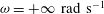 ${\it\omega}=+\infty ~\text{rad}~\text{s}^{-1}$
, the point with coordinates
${\it\omega}=+\infty ~\text{rad}~\text{s}^{-1}$
, the point with coordinates
 $(-1,0)$
should be ‘encircled’ twice in the anticlockwise direction for the controller to stabilise the plant. Figure 12 shows that this is the case for the scaled open-loop system, which shows that there exists a so-called ‘gain window’, where proportional control stabilises the ROM. We therefore also implement a proportional controller and compare its performance with the robust controller. The design of the proportional controller is discussed in § 4.2. The shaped system also stabilises the ROM in this case, although we emphasise that this is only an intermediate step and that the aim of this initial procedure is to improve the robustness of the final controller iteratively and not to obtain the best possible controller using only classical loop-shaping.
$(-1,0)$
should be ‘encircled’ twice in the anticlockwise direction for the controller to stabilise the plant. Figure 12 shows that this is the case for the scaled open-loop system, which shows that there exists a so-called ‘gain window’, where proportional control stabilises the ROM. We therefore also implement a proportional controller and compare its performance with the robust controller. The design of the proportional controller is discussed in § 4.2. The shaped system also stabilises the ROM in this case, although we emphasise that this is only an intermediate step and that the aim of this initial procedure is to improve the robustness of the final controller iteratively and not to obtain the best possible controller using only classical loop-shaping.
4.1.2 Robustness optimisation step
The aim of the second step is to optimise the shaped system’s robustness, as quantified by the generalised stability margin
 $b$
, defined formally in appendix B. If the controller does not stabilise the plant, then
$b$
, defined formally in appendix B. If the controller does not stabilise the plant, then
 $b=0$
, and as the robustness increases,
$b=0$
, and as the robustness increases,
 $b\rightarrow 1$
. A minimum value of
$b\rightarrow 1$
. A minimum value of
 $0.2\leqslant b\leqslant 0.3$
is usually considered to be acceptable. As implied by its name,
$0.2\leqslant b\leqslant 0.3$
is usually considered to be acceptable. As implied by its name,
 $b$
is a generalisation of the standard gain and phase margins used in classical control. It gives a measure of both the robust performance and robust stability characteristics of a given (shaped) model and is also applicable to multiple-input–multiple-output systems.
$b$
is a generalisation of the standard gain and phase margins used in classical control. It gives a measure of both the robust performance and robust stability characteristics of a given (shaped) model and is also applicable to multiple-input–multiple-output systems.
The shaped plant
 $WG$
was therefore used as an initial condition for the
$WG$
was therefore used as an initial condition for the
 $\mathscr{H}_{\infty }$
loop-shaping algorithm. This resulted in a robust
$\mathscr{H}_{\infty }$
loop-shaping algorithm. This resulted in a robust
 $11$
th-order controller
$11$
th-order controller
 $K_{0}(s)=K_{\infty }(s)W(s)$
. High-order controllers are less easily implemented in practice and also less reliable, so it is desirable to keep the order of the controller as low as possible without excessively compromising the closed-loop performance. The
$K_{0}(s)=K_{\infty }(s)W(s)$
. High-order controllers are less easily implemented in practice and also less reliable, so it is desirable to keep the order of the controller as low as possible without excessively compromising the closed-loop performance. The
 $K_{\infty }$
part of the controller was thus subsequently reduced using matlab’s balreal and modred commands, resulting in a final eighth-order controller
$K_{\infty }$
part of the controller was thus subsequently reduced using matlab’s balreal and modred commands, resulting in a final eighth-order controller
 $K(s)=K_{\infty ,r}(s)W(s)$
. The generalised stability margins for the optimised and reduced controllers are
$K(s)=K_{\infty ,r}(s)W(s)$
. The generalised stability margins for the optimised and reduced controllers are
 $b(WG,K_{\infty })=0.427$
and
$b(WG,K_{\infty })=0.427$
and
 $b(WG,K_{\infty ,r})=0.422$
, respectively, which shows first that the robustness of the
$b(WG,K_{\infty ,r})=0.422$
, respectively, which shows first that the robustness of the
 $\mathscr{H}_{\infty }$
controller is satisfactory, and second that the order reduction process only deteriorated this robustness very marginally.
$\mathscr{H}_{\infty }$
controller is satisfactory, and second that the order reduction process only deteriorated this robustness very marginally.
4.2 Proportional control
In order to compare the
 $\mathscr{H}_{\infty }$
loop-shaping approach to the proportional control approach used in several classical studies such as Roussopoulos (Reference Roussopoulos1993) and Park, Ladd & Hendricks (Reference Park, Ladd and Hendricks1994), we also design a proportional controller:
$\mathscr{H}_{\infty }$
loop-shaping approach to the proportional control approach used in several classical studies such as Roussopoulos (Reference Roussopoulos1993) and Park, Ladd & Hendricks (Reference Park, Ladd and Hendricks1994), we also design a proportional controller:
 $u(s)=K_{P}\,y(s)$
if
$u(s)=K_{P}\,y(s)$
if
 $r(s)=0$
, where
$r(s)=0$
, where
 $K_{P}$
is simply a constant. As mentioned above, it was found that there exists a ‘gain window’, where proportional control can be expected to stabilise the ROM. In a similar manner to Illingworth et al. (Reference Illingworth, Naito and Fukagata2014), we use our ERA model to select an adequate
$K_{P}$
is simply a constant. As mentioned above, it was found that there exists a ‘gain window’, where proportional control can be expected to stabilise the ROM. In a similar manner to Illingworth et al. (Reference Illingworth, Naito and Fukagata2014), we use our ERA model to select an adequate
 $K_{P}$
value. Here, we choose to maximise robustness, as quantified by
$K_{P}$
value. Here, we choose to maximise robustness, as quantified by
 $b(K_{P}G,1)$
, in order to show that this stability and performance parameter is useful even for very simple controller design strategies. The optimal value was found to correspond to
$b(K_{P}G,1)$
, in order to show that this stability and performance parameter is useful even for very simple controller design strategies. The optimal value was found to correspond to
 $K_{P}\approx 21$
, for which
$K_{P}\approx 21$
, for which
 $b(K_{P}G,1)=0.180$
. This value is smaller than
$b(K_{P}G,1)=0.180$
. This value is smaller than
 $b(WG,K_{\infty r})=0.422$
, indicating that the
$b(WG,K_{\infty r})=0.422$
, indicating that the
 $\mathscr{H}_{\infty }$
loop-shaping controller can be expected to be more robust than the proportional controller. This is further discussed in the next section.
$\mathscr{H}_{\infty }$
loop-shaping controller can be expected to be more robust than the proportional controller. This is further discussed in the next section.
4.3 Controller robustness and model uncertainty
In order to obtain the reference model that was used for controller design in §§ 4.1 and 4.2, we selected one of three modelling algorithms, a final simulation time of
 $t_{\infty }=50$
convective time units and a model order of
$t_{\infty }=50$
convective time units and a model order of
 $r=10$
. In this section, we show that robust control tools can quantify the model uncertainty associated with these choices. A related approach was used by Jones et al. (Reference Jones, Heins, Kerrigan, Morrison and Sharma2015) in a grid refinement study.
$r=10$
. In this section, we show that robust control tools can quantify the model uncertainty associated with these choices. A related approach was used by Jones et al. (Reference Jones, Heins, Kerrigan, Morrison and Sharma2015) in a grid refinement study.
A useful tool that naturally fits in the
 $\mathscr{H}_{\infty }$
loop-shaping framework is the
$\mathscr{H}_{\infty }$
loop-shaping framework is the
 ${\it\nu}$
-gap metric introduced by Vinnicombe (Reference Vinnicombe1993) and denoted by
${\it\nu}$
-gap metric introduced by Vinnicombe (Reference Vinnicombe1993) and denoted by
 ${\it\delta}_{{\it\nu}}$
. It provides a measure of how differently two systems shaped with the same weights
${\it\delta}_{{\it\nu}}$
. It provides a measure of how differently two systems shaped with the same weights
 $W(s)$
can be expected to behave in closed loop. The
$W(s)$
can be expected to behave in closed loop. The
 ${\it\nu}$
-gap takes a value between 0 and 1 (
${\it\nu}$
-gap takes a value between 0 and 1 (
 ${\it\delta}_{{\it\nu}}=0$
between identical models) and it is formally defined in appendix B. This metric can be used to provide stability guarantees for uncertain systems. Specifically, if
${\it\delta}_{{\it\nu}}=0$
between identical models) and it is formally defined in appendix B. This metric can be used to provide stability guarantees for uncertain systems. Specifically, if
 $b(WG,K_{\infty })>{\it\delta}_{{\it\nu}}(WG,WG_{i})$
for given
$b(WG,K_{\infty })>{\it\delta}_{{\it\nu}}(WG,WG_{i})$
for given
 $W$
and
$W$
and
 $K_{\infty }$
, and for a ‘perturbed’ model
$K_{\infty }$
, and for a ‘perturbed’ model
 $G_{i}$
, then the controller
$G_{i}$
, then the controller
 $K_{0}=K_{\infty }W$
also stabilises
$K_{0}=K_{\infty }W$
also stabilises
 $G_{i}$
. For any perturbed model where
$G_{i}$
. For any perturbed model where
 $b(WG,K_{\infty })<{\it\delta}_{{\it\nu}}(WG,WG_{i})$
, the stability of the perturbed closed-loop model can be checked by calculating
$b(WG,K_{\infty })<{\it\delta}_{{\it\nu}}(WG,WG_{i})$
, the stability of the perturbed closed-loop model can be checked by calculating
 $b(WG_{i},K_{\infty })$
.
$b(WG_{i},K_{\infty })$
.
As summarised in table 2, several ‘perturbed’ open-loop models
 $G_{i}$
were constructed by varying the model order, final simulation time and modelling method used. For all models, the
$G_{i}$
were constructed by varying the model order, final simulation time and modelling method used. For all models, the
 ${\it\nu}$
-gap metric corresponding both to the
${\it\nu}$
-gap metric corresponding both to the
 $\mathscr{H}_{\infty }$
loop-shaping weights
$\mathscr{H}_{\infty }$
loop-shaping weights
 ${\it\delta}_{{\it\nu}}(WG,WG_{i})$
and to the proportional controller
${\it\delta}_{{\it\nu}}(WG,WG_{i})$
and to the proportional controller
 ${\it\delta}_{{\it\nu}}(K_{P}G,K_{P}G_{i})$
were calculated and are shown in table 2.
${\it\delta}_{{\it\nu}}(K_{P}G,K_{P}G_{i})$
were calculated and are shown in table 2.
Table 2. Parameters used to generate the considered family of ‘perturbed’ models
 $G_{i}$
for the wake velocity sensor, and values of the corresponding
$G_{i}$
for the wake velocity sensor, and values of the corresponding
 ${\it\nu}$
-gap metric, calculated for both the robust controller weights and the proportional controller.
${\it\nu}$
-gap metric, calculated for both the robust controller weights and the proportional controller.

The
 ${\it\nu}$
-gap values in table 2 demonstrate the advantage of using
${\it\nu}$
-gap values in table 2 demonstrate the advantage of using
 $\mathscr{H}_{\infty }$
loop-shaping: although the
$\mathscr{H}_{\infty }$
loop-shaping: although the
 ${\it\nu}$
-gap associated with all models is similar for both controllers,
${\it\nu}$
-gap associated with all models is similar for both controllers,
 $b(WG,K_{\infty })>{\it\delta}_{{\it\nu}}(WG,WG_{i})$
for all
$b(WG,K_{\infty })>{\it\delta}_{{\it\nu}}(WG,WG_{i})$
for all
 $i$
, whereas this is not the case with the proportional controller. The robust controller is thus guaranteed to stabilise all the models considered here. On the other hand, it was necessary to verify that the proportional controller in fact does stabilise
$i$
, whereas this is not the case with the proportional controller. The robust controller is thus guaranteed to stabilise all the models considered here. On the other hand, it was necessary to verify that the proportional controller in fact does stabilise
 $G_{BPOD}$
by checking that
$G_{BPOD}$
by checking that
 $b(K_{P}G_{BPOD},1)>0$
since
$b(K_{P}G_{BPOD},1)>0$
since
 $b(K_{P}G,1)<{\it\delta}_{{\it\nu}}(K_{P}G,K_{P}G_{BPOD})$
. It was found that
$b(K_{P}G,1)<{\it\delta}_{{\it\nu}}(K_{P}G,K_{P}G_{BPOD})$
. It was found that
 $b(K_{P}G_{BPOD},1)=0.144$
.
$b(K_{P}G_{BPOD},1)=0.144$
.
Table 2 also shows that models obtained with a larger final simulation time or order have a very small
 ${\it\nu}$
-gap so they can be expected to behave in a similar manner to the reference model, whereas larger differences appear with lower
${\it\nu}$
-gap so they can be expected to behave in a similar manner to the reference model, whereas larger differences appear with lower
 $t_{\infty }$
and
$t_{\infty }$
and
 $r$
values. This suggests that our chosen
$r$
values. This suggests that our chosen
 $t_{\infty }$
and
$t_{\infty }$
and
 $r$
values are allowing us to obtain a converged model and resolve most of the important dynamics of the input–output system. Similarly, the distance between the two ERA models is negligible, which confirms that the early impulse response of the nonlinear flow provides adequate information to obtain a useful ERA model. Finally, a non-negligible value of
$r$
values are allowing us to obtain a converged model and resolve most of the important dynamics of the input–output system. Similarly, the distance between the two ERA models is negligible, which confirms that the early impulse response of the nonlinear flow provides adequate information to obtain a useful ERA model. Finally, a non-negligible value of
 ${\it\delta}_{{\it\nu}}$
is obtained with
${\it\delta}_{{\it\nu}}$
is obtained with
 $G_{BPOD}$
. This indicates that the ROMs may be sensitive to the modelling approach in this case and that, with the chosen weights
$G_{BPOD}$
. This indicates that the ROMs may be sensitive to the modelling approach in this case and that, with the chosen weights
 $W$
and
$W$
and
 $K_{P}$
, some differences can be expected between the responses of the two models in closed loop. Nevertheless, the model
$K_{P}$
, some differences can be expected between the responses of the two models in closed loop. Nevertheless, the model
 $G_{BPOD}$
is still stabilised by both controllers.
$G_{BPOD}$
is still stabilised by both controllers.
We emphasise that these tests are all performed a priori, in the sense that no closed-loop simulation is required. They suggest that the full-order flow and the ROMs are likely to behave in a similar manner since the stability and performance of the closed loop are suitably robust to the modelling technique and model parameters. This analysis is equally instructive for controllers designed explicitly using robust control methods such as
 $K(s)$
and for much simpler controllers such as
$K(s)$
and for much simpler controllers such as
 $K_{P}$
.
$K_{P}$
.
4.4 Body-mounted force sensor: modelling and controller design
The same procedure was then followed using the body-mounted force sensor introduced in § 2: first a
 $10$
th-order ERA model was obtained by scaling the response of the full nonlinear flow field to a small impulse. Note that the two sensor signals were recorded at the same time so it was not necessary to run a new simulation to obtain this model. In fact, the measurements from an arbitrary number of candidate sensors can be stored simultaneously for a given actuator configuration. As a result, there is effectively no added cost associated with the construction and comparison of models obtained with a large number of sensors. An ERA model was therefore also obtained from the fully linear response using this sensor.
$10$
th-order ERA model was obtained by scaling the response of the full nonlinear flow field to a small impulse. Note that the two sensor signals were recorded at the same time so it was not necessary to run a new simulation to obtain this model. In fact, the measurements from an arbitrary number of candidate sensors can be stored simultaneously for a given actuator configuration. As a result, there is effectively no added cost associated with the construction and comparison of models obtained with a large number of sensors. An ERA model was therefore also obtained from the fully linear response using this sensor.
A robust stabilising controller was then designed by shaping the Nyquist diagram with a first-order lag filter and a first-order low-pass filter. In this case, we note that, at this intermediate stage in the robust controller design process, the chosen weights
 $W(s)$
in fact do not stabilise the open-loop model. The robustness of the shaped system
$W(s)$
in fact do not stabilise the open-loop model. The robustness of the shaped system
 $WG$
was then improved using
$WG$
was then improved using
 $\mathscr{H}_{\infty }$
loop-shaping. The stability margins corresponding to the resulting
$\mathscr{H}_{\infty }$
loop-shaping. The stability margins corresponding to the resulting
 $14$
th-order controller and the eighth-order reduced controller are
$14$
th-order controller and the eighth-order reduced controller are
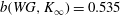 $b(WG,K_{\infty })=0.535$
and
$b(WG,K_{\infty })=0.535$
and
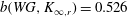 $b(WG,K_{\infty ,r})=0.526$
, respectively. The corresponding Nyquist diagrams are shown in figure 13. Note that the robust shaped systems
$b(WG,K_{\infty ,r})=0.526$
, respectively. The corresponding Nyquist diagrams are shown in figure 13. Note that the robust shaped systems
 $K_{0}G$
and
$K_{0}G$
and
 $KG$
have a peak at
$KG$
have a peak at
 ${\it\omega}\approx 0.78~\text{rad}~\text{s}^{-1}$
so their Nyquist diagrams have a large magnitude close to this frequency.
${\it\omega}\approx 0.78~\text{rad}~\text{s}^{-1}$
so their Nyquist diagrams have a large magnitude close to this frequency.
Using the force sensor configuration, it was noticed that the range of stabilising proportional gains was greatly reduced due to the fact that proportional control triggered instabilities at frequencies close to the time-stepping frequency. In order to circumvent this numerical issue, the proportional controller was first coupled with a simple second-order low-pass filter. The filter has a cutoff frequency of
 ${\it\omega}=200~\text{rad}~\text{s}^{-1}$
, and hence has no effect on the frequencies where physical phenomena take place in the flow. The final controller can therefore still be considered to be effectively a proportional controller. With this added filter, it was possible to identify a ‘gain window’ where a stability margin of
${\it\omega}=200~\text{rad}~\text{s}^{-1}$
, and hence has no effect on the frequencies where physical phenomena take place in the flow. The final controller can therefore still be considered to be effectively a proportional controller. With this added filter, it was possible to identify a ‘gain window’ where a stability margin of
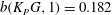 $b(K_{P}G,1)=0.182$
was obtained by using a scaling factor of
$b(K_{P}G,1)=0.182$
was obtained by using a scaling factor of
 $555$
. The model shaped with this controller
$555$
. The model shaped with this controller
 $K_{P}$
is also shown in figure 13.
$K_{P}$
is also shown in figure 13.

Figure 13. Controller design for the body-mounted force sensor, showing the Nyquist diagram of the (linear) ERA ROM in series with the proportional controller (
 $-K_{P}G$
), the manually shaped model (
$-K_{P}G$
), the manually shaped model (
 $-WG$
), the robust model (
$-WG$
), the robust model (
 $-K_{0}G$
) and the reduced robust model (
$-K_{0}G$
) and the reduced robust model (
 $-KG$
). The point with coordinates
$-KG$
). The point with coordinates
 $(-1,0)$
is shown by a cross. The locations corresponding to frequencies of
$(-1,0)$
is shown by a cross. The locations corresponding to frequencies of
 ${\it\omega}=0.6~\text{rad}~\text{s}^{-1}$
(▵),
${\it\omega}=0.6~\text{rad}~\text{s}^{-1}$
(▵),
 $0.7~\text{rad}~\text{s}^{-1}$
(▫),
$0.7~\text{rad}~\text{s}^{-1}$
(▫),
 $0.8~\text{rad}~\text{s}^{-1}$
(
$0.8~\text{rad}~\text{s}^{-1}$
(
 $\star$
), and
$\star$
), and
 $0.9~\text{rad}~\text{s}^{-1}$
(○) are also shown. Note that the minus signs are due to the positive feedback sign convention.
$0.9~\text{rad}~\text{s}^{-1}$
(○) are also shown. Note that the minus signs are due to the positive feedback sign convention.

Figure 14. Control using the wake velocity sensor connected in closed loop with the two considered controllers: (a) output and (b) input corresponding to the closed-loop impulse response predicted by the ROM from § 3.4 and compared with the full linearised impulse response at
 $Re=80$
. In all cases the system is subject to an impulse at
$Re=80$
. In all cases the system is subject to an impulse at
 $t=0$
and the controller is switched on after
$t=0$
and the controller is switched on after
 $t=50$
convective time units.
$t=50$
convective time units.
Table 3. Parameters used to generate the considered family of ‘perturbed’ models
 $G_{i}$
for the body-mounted force sensor, and values of the corresponding
$G_{i}$
for the body-mounted force sensor, and values of the corresponding
 ${\it\nu}$
-gap metric, calculated for both the robust controller weights and the proportional controller.
${\it\nu}$
-gap metric, calculated for both the robust controller weights and the proportional controller.

Table 3 shows the
 ${\it\nu}$
-gap corresponding to the robust controller weights
${\it\nu}$
-gap corresponding to the robust controller weights
 $W$
and the proportional controller
$W$
and the proportional controller
 $K_{P}$
for all considered models for the force sensor. The results are similar to those in table 2, although the
$K_{P}$
for all considered models for the force sensor. The results are similar to those in table 2, although the
 ${\it\nu}$
-gap values are overall slightly higher. As with the velocity sensor,
${\it\nu}$
-gap values are overall slightly higher. As with the velocity sensor,
 $b(WG,K_{\infty ,r})>{\it\delta}_{{\it\nu}}(WG,WG_{i})$
for all
$b(WG,K_{\infty ,r})>{\it\delta}_{{\it\nu}}(WG,WG_{i})$
for all
 $G_{i}$
with the robust controller. With the proportional controller, on the other hand,
$G_{i}$
with the robust controller. With the proportional controller, on the other hand,
 $b(K_{P}G,1)<{\it\delta}_{{\it\nu}}(K_{P}G,K_{P}G_{t_{\infty }=25})$
. The stability of the perturbed closed-loop model was thus checked and it was found that
$b(K_{P}G,1)<{\it\delta}_{{\it\nu}}(K_{P}G,K_{P}G_{t_{\infty }=25})$
. The stability of the perturbed closed-loop model was thus checked and it was found that
 $b(K_{P}G_{t_{\infty }=25},1)=0.202>0$
.
$b(K_{P}G_{t_{\infty }=25},1)=0.202>0$
.
This analysis again confirms that the closed loop is not excessively sensitive to the chosen modelling technique and model parameters. We can therefore confidently proceed to implement the controllers in the full-order flow.
4.5 Controller performance
Equipped with robust stabilising controllers, three increasingly demanding tests were performed for the four considered control configurations. The results are presented in this section.
4.5.1 Closed-loop response predictions
First, the closed-loop response predicted by each ROM was compared to that of the full linearised system: the flow was forced with an impulse and allowed to evolve for 50 convective time units, thus allowing the unstable modes to develop before the controllers are switched on. In figure 14 the response predicted by the ROM (velocity sensor) is compared to the full linearised system’s response in closed loop. With both controllers, the two responses match very closely, even after the controller is switched on. Note also that the proportional controller leads to a slower stabilisation of the flow in this case.
Similar conclusions can be drawn from the results obtained with the body-mounted force sensor, shown in figure 15. In this case, the convergence rate of the output signal is lower and it therefore takes longer for the flow to return to its unstable equilibrium state. On the other hand, the initial response of the controller is less aggressive than with the wake velocity sensor. Again, the stabilisation of the flow is faster with
 $K$
than with
$K$
than with
 $K_{P}$
.
$K_{P}$
.

Figure 15. Control using the body-mounted force sensor connected in closed loop with the two considered controllers: (a) output and (b) input corresponding to the closed-loop impulse response predicted by the ROM (identified with the ERA based on nonlinear dynamics and with the body-mounted force sensor) and compared with the full linearised impulse response at
 $Re=80$
. In all cases the system is subject to an impulse at
$Re=80$
. In all cases the system is subject to an impulse at
 $t=0$
and the controller is switched on after
$t=0$
and the controller is switched on after
 $t=50$
convective time units.
$t=50$
convective time units.
4.5.2 Robustness to nonlinear initial conditions
The robustness of the controllers to nonlinear effects was then tested. After triggering the instability with an impulse, the nonlinear flow was left to evolve to its limit-cycling (vortex shedding) state. The controllers were only switched on when vortex shedding was fully established (after 200 convective time units). We emphasise that neither the models nor the controllers incorporate any information about the limit-cycle dynamics, which do not even necessarily evolve about the same state as the base flow.
However, as shown in figures 16 and 17, the two proportional controllers and the two
 $\mathscr{H}_{\infty }$
controllers are robust enough to stabilise the flow. Figure 18 shows the evolution of the forces on the body in all four configurations: starting from their base flow values, the instability is triggered and the forces evolve as the flow reaches the limit cycle. Once the controllers have been switched on, the forces quickly return to the base flow values.
$\mathscr{H}_{\infty }$
controllers are robust enough to stabilise the flow. Figure 18 shows the evolution of the forces on the body in all four configurations: starting from their base flow values, the instability is triggered and the forces evolve as the flow reaches the limit cycle. Once the controllers have been switched on, the forces quickly return to the base flow values.
In fact, the entire closed-loop flow returns to a state that is close to the low-drag unstable steady state in all cases. Figure 19 shows snapshots of the flow field (controlled using the robust controller associated with the body-mounted force sensor) at the moment when the control is switched on (after
 $t=200$
convective time units), and then as the flow is gradually stabilised. After
$t=200$
convective time units), and then as the flow is gradually stabilised. After
 $500$
convective time units (figure 19
d), the vortex shedding is effectively fully suppressed and the flow is similar to the base state in figure 2.
$500$
convective time units (figure 19
d), the vortex shedding is effectively fully suppressed and the flow is similar to the base state in figure 2.
For the wake velocity sensor, the convergence of the forces takes place at a similar rate with both controllers. As in the linear framework in § 4.5.1, the flow takes longer to converge to its steady state with the body-mounted force sensor configuration. However, in this case, the proportional controller leads to a faster flow stabilisation than the robust controller.
Overall, these results thus show that the designed controllers are robust to significant nonlinear effects for all four configurations.

Figure 16. (a) Output and (b) input corresponding to the closed-loop response of the full nonlinear system at
 $Re=80$
, using the wake velocity sensor and the two corresponding controllers. The system is subject to an impulse at
$Re=80$
, using the wake velocity sensor and the two corresponding controllers. The system is subject to an impulse at
 $t=0$
and the controllers are switched on after
$t=0$
and the controllers are switched on after
 $t=200$
convective time units.
$t=200$
convective time units.

Figure 17. (a) Output and (b) input corresponding to the closed-loop response of the full nonlinear system at
 $Re=80$
, using the body-mounted force sensor and the two corresponding controllers. The system is subject to an impulse at
$Re=80$
, using the body-mounted force sensor and the two corresponding controllers. The system is subject to an impulse at
 $t=0$
and the controllers are switched on after
$t=0$
and the controllers are switched on after
 $t=200$
convective time units.
$t=200$
convective time units.

Figure 18. (a) Lift and (b) drag force coefficients corresponding to the closed-loop response of the full nonlinear system at
 $Re=80$
. The drag coefficient of the base flow is also shown in panel (b). The system is subject to an impulse at
$Re=80$
. The drag coefficient of the base flow is also shown in panel (b). The system is subject to an impulse at
 $t=0$
and the controllers are switched on at
$t=0$
and the controllers are switched on at
 $t=200$
convective time units. The results obtained with all four sensor–controller configurations are shown.
$t=200$
convective time units. The results obtained with all four sensor–controller configurations are shown.

Figure 19. Snapshots of the controlled flow field (using the body-mounted force sensor and the robust controller) after (a)
 $t=200$
convective time units when the control is turned on, and then at (b)
$t=200$
convective time units when the control is turned on, and then at (b)
 $t=300$
, (c)
$t=300$
, (c)
 $t=400$
, and (d)
$t=400$
, and (d)
 $t=500$
convective time units. Vorticity contours are shown; negative contours are bounded by a line. Contour levels are from
$t=500$
convective time units. Vorticity contours are shown; negative contours are bounded by a line. Contour levels are from
 $-1.8$
to
$-1.8$
to
 $1.8$
in increments of
$1.8$
in increments of
 $0.4$
.
$0.4$
.
4.5.3 Robustness to changes in the Reynolds number
The controllers were then challenged further by repeating the test from § 4.5.2 but with larger (and hence off-design) Reynolds number values of
 $Re=90$
and
$Re=90$
and
 $100$
. This introduces additional modifications in the dynamics of the flows that the controllers are attempting to stabilise. In particular, the flow becomes more unstable at higher
$100$
. This introduces additional modifications in the dynamics of the flows that the controllers are attempting to stabilise. In particular, the flow becomes more unstable at higher
 $Re$
values and is hence harder to control.
$Re$
values and is hence harder to control.
It was found that, using the body-mounted force sensor, neither controller was able to fully stabilise the flow at
 $Re=90$
or
$Re=90$
or
 $100$
. With the velocity sensor configuration (and with both of the associated controllers), the flow was fully stabilised from the limit cycle at
$100$
. With the velocity sensor configuration (and with both of the associated controllers), the flow was fully stabilised from the limit cycle at
 $Re=90$
and
$Re=90$
and
 $100$
. Further simulations were run at
$100$
. Further simulations were run at
 $Re=110$
,
$Re=110$
,
 $130$
and
$130$
and
 $150$
: the flow was found to be stabilised from the limit cycle at
$150$
: the flow was found to be stabilised from the limit cycle at
 $Re=110$
with the robust controller and almost fully with the proportionally controller. At
$Re=110$
with the robust controller and almost fully with the proportionally controller. At
 $Re=130$
, neither controller fully stabilised the flow.
$Re=130$
, neither controller fully stabilised the flow.
Even in cases where the flow was not fully stabilised, the control was found to result in a positive net energy gain, as measured by the total average power required to drive the body through the fluid (after transients). The instantaneous total power can be expressed as the sum of the power required to overcome the drag
 $D(t)$
and the power supplied to the fluid by the actuators (see e.g. Frohnapfel, Hasegawa & Quadrio Reference Frohnapfel, Hasegawa and Quadrio2012). In non-dimensional form, this can be written as
$D(t)$
and the power supplied to the fluid by the actuators (see e.g. Frohnapfel, Hasegawa & Quadrio Reference Frohnapfel, Hasegawa and Quadrio2012). In non-dimensional form, this can be written as
 $$\begin{eqnarray}\displaystyle \frac{P_{total}(t)}{\frac{1}{2}{\it\rho}U_{\infty }^{3}H} & = & \displaystyle \frac{D(t)U_{\infty }}{\frac{1}{2}{\it\rho}U_{\infty }^{3}H}+\frac{P_{control}(t)}{\frac{1}{2}{\it\rho}U_{\infty }^{3}H}\nonumber\\ \displaystyle & = & \displaystyle C_{D}+\int _{A_{F}}\left[\frac{\boldsymbol{f}(t)}{\frac{1}{2}{\it\rho}U_{\infty }^{2}H}\boldsymbol{\cdot }\frac{\boldsymbol{u}(t)}{U_{\infty }}\right]\,\text{d}A_{F},\end{eqnarray}$$
where
 $P_{total}(t)$
and
$P_{total}(t)$
and
 $P_{control}(t)$
are the dimensional total and control power per unit width, respectively,
$P_{control}(t)$
are the dimensional total and control power per unit width, respectively,
 ${\it\rho}$
is the fluid density,
${\it\rho}$
is the fluid density,
 $A_{F}$
is the area where the forcing is applied,
$A_{F}$
is the area where the forcing is applied,
 $\boldsymbol{f}$
is the local dimensional force per unit area and
$\boldsymbol{f}$
is the local dimensional force per unit area and
 $\boldsymbol{u}$
is the local dimensional velocity. Note that, in practice, an actuator model would be desirable in order to obtain a more realistic estimate of the required input power.
$\boldsymbol{u}$
is the local dimensional velocity. Note that, in practice, an actuator model would be desirable in order to obtain a more realistic estimate of the required input power.
In our case, the control power (second term) tends to zero when the flow is fully stabilised. Moreover, in all cases where the control input converges to a finite value, it was found that the time-averaged value of
 $P_{control}$
after transients was at most of the order of a hundredth of a per cent of
$P_{control}$
after transients was at most of the order of a hundredth of a per cent of
 $P_{total}$
and usually much less. This negligible value is due to the fact that the flow is almost symmetric at the actuation location while the forcing is purely antisymmetric. As a result, changes in the converged drag coefficient can be directly linked to changes in the total required power. The results are shown in figure 20: clearly in all cases, the required time-averaged converged power is reduced significantly. For the wake velocity sensor, the robust controller leads to a great power reduction than the proportional controller. This general trend seems to be inverted for the body-mounted force sensor.
$P_{total}$
and usually much less. This negligible value is due to the fact that the flow is almost symmetric at the actuation location while the forcing is purely antisymmetric. As a result, changes in the converged drag coefficient can be directly linked to changes in the total required power. The results are shown in figure 20: clearly in all cases, the required time-averaged converged power is reduced significantly. For the wake velocity sensor, the robust controller leads to a great power reduction than the proportional controller. This general trend seems to be inverted for the body-mounted force sensor.
The results from this test suggest that the velocity sensor configuration is in general more robust to an increase in the Reynolds number than the force sensor configuration, despite the fact that the stability margin is larger with the body-mounted sensor. This implies that the dynamics of the shaped system experience larger changes with the force sensor than with the velocity sensor. As the Reynolds number is increased, Giannetti & Luchini (Reference Giannetti and Luchini2007) have shown that the wavemaker region in a cylinder wake at low Reynolds numbers becomes elongated and shifts further downstream. Since the body-mounted sensor is located in a less observable region of the flow (see figure 4) and is already on the upstream edge of the wavemaker region at the design Reynolds number (see figure 5), this could explain why the associated input–output dynamics are more strongly affected by an increase in the Reynolds number.

Figure 20. Comparison of the total power required to drive the body through the fluid in the unstable equilibrium flow state, the unforced vortex shedding state and with the two controllers, for cases where the flow is not fully stabilised with (a) the body-mounted force sensor and (b) the wake velocity sensor.
4.5.4 Further comments
In § 4.3, it was found that
 $\mathscr{H}_{\infty }$
loop-shaping yields controllers that are expected to be considerably more robust than proportional controllers (as quantified by
$\mathscr{H}_{\infty }$
loop-shaping yields controllers that are expected to be considerably more robust than proportional controllers (as quantified by
 $b$
). Additionally, the window of stabilising proportional gains eventually disappears for sufficiently large
$b$
). Additionally, the window of stabilising proportional gains eventually disappears for sufficiently large
 $Re$
and in this case a dynamic controller is necessary to stabilise the flow (e.g. Illingworth et al.
Reference Illingworth, Naito and Fukagata2014). Nevertheless, the results from this section indicate that, in cases where a gain window does exist, choosing the proportional control gain that maximises the generalised stability margin can result in controllers whose robustness and performance are in practice similar to that of
$Re$
and in this case a dynamic controller is necessary to stabilise the flow (e.g. Illingworth et al.
Reference Illingworth, Naito and Fukagata2014). Nevertheless, the results from this section indicate that, in cases where a gain window does exist, choosing the proportional control gain that maximises the generalised stability margin can result in controllers whose robustness and performance are in practice similar to that of
 $\mathscr{H}_{\infty }$
loop-shaping controllers. The generalised stability margin
$\mathscr{H}_{\infty }$
loop-shaping controllers. The generalised stability margin
 $b$
therefore appears to be a useful parameter to guide the design of stabilising controllers for fluid flows in general. We note however that
$b$
therefore appears to be a useful parameter to guide the design of stabilising controllers for fluid flows in general. We note however that
 $b$
should not be used blindly: although the force sensor robust controller provided in the largest stability margin, this system was not the most robust to an increase in the Reynolds number.
$b$
should not be used blindly: although the force sensor robust controller provided in the largest stability margin, this system was not the most robust to an increase in the Reynolds number.
Compared to other studies where proportional and/or classical control was used (e.g. Roussopoulos Reference Roussopoulos1993; Park et al.
Reference Park, Ladd and Hendricks1994), the availability of an accurate input–output model enables the use of
 $b$
to select a proportional controller gain value that provides good robustness. This information is not available when tuning a controller manually.
$b$
to select a proportional controller gain value that provides good robustness. This information is not available when tuning a controller manually.
It is also important to note that the controllers used in this study were designed in part manually. This iterative procedure is different for each actuator–sensor configuration and may be better optimised in this case with one of the sensor configurations than the other. As a result, the comparison between the two sensors cannot be made quantitatively.
Additionally, recall that the purpose of the simulations performed here was to test the robustness of fixed controllers as the Reynolds number takes on larger off-design values. The aim was therefore not to identify the highest value of the Reynolds number for which flow stabilisation is possible, as optimal control techniques would be better suited for such a study (see for instance Lauga & Bewley Reference Lauga and Bewley2003).
5 Conclusions
This paper has shown that it is straightforward and justified to obtain linear low-order models for the dynamics of fluid flows about an unstable equilibrium state, by directly applying the ERA to the system’s impulse response. The resulting models were shown to be capable of predicting the transient and long-term flow dynamics in open loop and in closed loop. They were also found to be sufficiently accurate to design robust stabilising controllers.
The method was applied to the unstable flow over a D-shaped body, with body-mounted actuators, and two sensor configurations. We first showed that, if projection-free BPOD is used to obtain the model as in Flinois et al. (Reference Flinois, Morgans and Schmid2015), then the analysis of actuator–sensor placement can be facilitated by extracting relevant information from the balanced modes. We then confirmed that the ERA can also be used at a much reduced cost and without the need for an adjoint solver, in order to obtain theoretically identical models, directly from the unstable system’s impulse response. In experiments or if a linearised solver is not available, it was shown that accurate models can also be obtained using the ERA, from the early, approximately linear, part of the impulse response of the full nonlinear flow. Such ERA ROMs, based on the nonlinear flow dynamics, were then used to design stabilising feedback controllers for two sensor configurations: one located in the wake and one mounted on the body surface.
Both proportional controllers and robust controllers based on the
 $\mathscr{H}_{\infty }$
loop-shaping procedure of McFarlane & Glover (Reference McFarlane and Glover1992) were designed. In both cases, it was found that robust control tools such as the generalised stability margin and the
$\mathscr{H}_{\infty }$
loop-shaping procedure of McFarlane & Glover (Reference McFarlane and Glover1992) were designed. In both cases, it was found that robust control tools such as the generalised stability margin and the
 ${\it\nu}$
-gap metric are particularly well suited to the design of robust stabilising controllers for unstable flows. These enable the analysis of the sensitivity of the closed-loop behaviour to the chosen modelling method and to model parameters such as the model order. They are central to the
${\it\nu}$
-gap metric are particularly well suited to the design of robust stabilising controllers for unstable flows. These enable the analysis of the sensitivity of the closed-loop behaviour to the chosen modelling method and to model parameters such as the model order. They are central to the
 $\mathscr{H}_{\infty }$
loop-shaping framework and were also found to provide an effective means to optimise the robustness of proportional controllers using the ERA models.
$\mathscr{H}_{\infty }$
loop-shaping framework and were also found to provide an effective means to optimise the robustness of proportional controllers using the ERA models.
Comparing the closed-loop response of the full-order linearised flow to the predictions made by the models showed that the ERA ROMs were sufficiently accurate to design stabilising controllers for the actual flow and also capable of predicting its closed-loop behaviour accurately. Furthermore, all controllers led to the full stabilisation of the nonlinear flow from the (unmodelled) vortex shedding limit cycle. Finally, it was found that the wake sensor was more robust to an increase in the Reynolds number than the body-mounted sensor.
All the key steps followed throughout this study can be performed with a standard nonlinear flow solver. This is a crucial point, as linearised and adjoint solvers are not available in a large number of relevant flow control scenarios. It also suggests that some experimental set-ups may benefit from this approach. In order to obtain models for unstable systems, previous studies have relied either on expensive computational techniques or on the difficult task of finding a stabilising controller for the flow, without a model for the dynamics. In contrast, the ERA is straightforward to implement and has a low computational cost. Here, we have shown that it can be used directly to construct models of high enough quality to design and implement robust stabilising controllers for unstable flows.
Acknowledgements
This research is funded by the UK Engineering and Physical Sciences Research Council (EPSRC). The authors also thank Professor T. Colonius from the California Institute of Technology for the immersed-boundary fractional step code on which the simulations presented here are based. All readers who are interested to obtain the data used in this paper are invited to email t.flinois11@imperial.ac.uk.
Appendix A. Eigensystem Realisation Algorithm for unstable flows
A.1 Projection-free approximate balanced truncation for unstable flows
This method assumes that the evolution of the system is linear-time-invariant (LTI) and can hence be described in state-space form. We will assume the system is discrete to make the comparison between this method and the ERA more straightforward in § A.2, but the problem can equivalently be formulated in continuous form. In fact, the continuous approach is the one implemented in the present work.
We thus assume the system is governed by:
 $$\begin{eqnarray}\displaystyle \left.\begin{array}{@{}c@{}}\boldsymbol{x}(k+1)=\unicode[STIX]{x1D63C}\boldsymbol{x}(k)+\unicode[STIX]{x1D63D}\boldsymbol{u}(k),\\ \boldsymbol{y}(k)=\unicode[STIX]{x1D63E}\boldsymbol{x}(k).\end{array}\right\} & & \displaystyle\end{eqnarray}$$
Here
 $\boldsymbol{x}\in \mathbb{C}^{n_{x}}$
is the state vector,
$\boldsymbol{x}\in \mathbb{C}^{n_{x}}$
is the state vector,
 $\boldsymbol{u}\in \mathbb{C}^{n_{u}}$
is the input vector,
$\boldsymbol{u}\in \mathbb{C}^{n_{u}}$
is the input vector,
 $\boldsymbol{y}\in \mathbb{C}^{n_{y}}$
is the output vector and the realisation of the system is defined by the matrices
$\boldsymbol{y}\in \mathbb{C}^{n_{y}}$
is the output vector and the realisation of the system is defined by the matrices
 $(\unicode[STIX]{x1D63C},\unicode[STIX]{x1D63D},\unicode[STIX]{x1D63E})$
of appropriate dimensions. The dynamics of the associated adjoint system can also be expressed in state-space form:
$(\unicode[STIX]{x1D63C},\unicode[STIX]{x1D63D},\unicode[STIX]{x1D63E})$
of appropriate dimensions. The dynamics of the associated adjoint system can also be expressed in state-space form:
 $$\begin{eqnarray}\displaystyle \left.\begin{array}{@{}c@{}}\boldsymbol{z}(k+1)=\unicode[STIX]{x1D63C}^{\dagger }\boldsymbol{z}(k)+\unicode[STIX]{x1D63E}^{\dagger }\boldsymbol{v}(k),\\ \boldsymbol{w}(k)=\unicode[STIX]{x1D63D}^{\dagger }\boldsymbol{z}(k).\end{array}\right\} & & \displaystyle\end{eqnarray}$$
The
 $^{\dagger }$
superscript refers to the complex conjugate transpose and in this case
$^{\dagger }$
superscript refers to the complex conjugate transpose and in this case
 $\boldsymbol{z}\in \mathbb{C}^{n_{x}}$
is the adjoint state vector,
$\boldsymbol{z}\in \mathbb{C}^{n_{x}}$
is the adjoint state vector,
 $\boldsymbol{v}\in \mathbb{C}^{n_{y}}$
is the adjoint input vector and
$\boldsymbol{v}\in \mathbb{C}^{n_{y}}$
is the adjoint input vector and
 $\boldsymbol{w}\in \mathbb{C}^{n_{u}}$
is the adjoint output vector. Note that, in general, the adjoint formulation is obtained based on a non-trivial inner-product matrix, but for clarity we assume the identity matrix is used here.
$\boldsymbol{w}\in \mathbb{C}^{n_{u}}$
is the adjoint output vector. Note that, in general, the adjoint formulation is obtained based on a non-trivial inner-product matrix, but for clarity we assume the identity matrix is used here.
The realisation
 $(\unicode[STIX]{x1D63C},\unicode[STIX]{x1D63D},\unicode[STIX]{x1D63E})$
of the primal system in (A 1) is not unique. Any appropriate coordinate transformation defined by the matrices
$(\unicode[STIX]{x1D63C},\unicode[STIX]{x1D63D},\unicode[STIX]{x1D63E})$
of the primal system in (A 1) is not unique. Any appropriate coordinate transformation defined by the matrices
 $\unicode[STIX]{x1D64F}$
and
$\unicode[STIX]{x1D64F}$
and
 $\unicode[STIX]{x1D64E}$
such that
$\unicode[STIX]{x1D64E}$
such that
 $\unicode[STIX]{x1D64F}=\unicode[STIX]{x1D64E}^{-1}$
can be applied to it, resulting in the transformed realisation
$\unicode[STIX]{x1D64F}=\unicode[STIX]{x1D64E}^{-1}$
can be applied to it, resulting in the transformed realisation
 $(\unicode[STIX]{x1D64E}\unicode[STIX]{x1D63C}\unicode[STIX]{x1D64F},\unicode[STIX]{x1D64E}\unicode[STIX]{x1D63D},\unicode[STIX]{x1D63E}\unicode[STIX]{x1D64F})$
, with unmodified input–output dynamics. The purpose of balanced truncation is to find the transformation that results in a transformed state vector
$(\unicode[STIX]{x1D64E}\unicode[STIX]{x1D63C}\unicode[STIX]{x1D64F},\unicode[STIX]{x1D64E}\unicode[STIX]{x1D63D},\unicode[STIX]{x1D63E}\unicode[STIX]{x1D64F})$
, with unmodified input–output dynamics. The purpose of balanced truncation is to find the transformation that results in a transformed state vector
 $\hat{\boldsymbol{x}}=\unicode[STIX]{x1D64F}\boldsymbol{x}$
, where the states are sorted in decreasing order of dynamical significance. The significance of a state in this context is affected both by the amount of input energy required to reach it from
$\hat{\boldsymbol{x}}=\unicode[STIX]{x1D64F}\boldsymbol{x}$
, where the states are sorted in decreasing order of dynamical significance. The significance of a state in this context is affected both by the amount of input energy required to reach it from
 $\hat{\boldsymbol{x}}=\mathbf{0}$
(its controllability) and the energy of the output signal generated by letting the system evolve with no input from that state (its observability). If such a transformation is found, the least significant states can easily be discarded by simply truncating the state vector and system matrices.
$\hat{\boldsymbol{x}}=\mathbf{0}$
(its controllability) and the energy of the output signal generated by letting the system evolve with no input from that state (its observability). If such a transformation is found, the least significant states can easily be discarded by simply truncating the state vector and system matrices.
Willcox & Peraire (Reference Willcox and Peraire2002) and Rowley (Reference Rowley2005) introduced a snapshot-based procedure that is based on the work of Moore (Reference Moore1981) and results in an approximation of the required transformation. It provides a set of so-called Hankel singular values (HSVs)
 ${\it\sigma}_{i}$
, sorted so that
${\it\sigma}_{i}$
, sorted so that
 ${\it\sigma}_{1}>\cdots >{\it\sigma}_{n_{x}}$
. They indicate how significant the corresponding state is. The algorithm is also referred to as balanced proper orthogonal decomposition (BPOD). The first step consists in storing state snapshots from the impulse response of the forward system into a matrix
${\it\sigma}_{1}>\cdots >{\it\sigma}_{n_{x}}$
. They indicate how significant the corresponding state is. The algorithm is also referred to as balanced proper orthogonal decomposition (BPOD). The first step consists in storing state snapshots from the impulse response of the forward system into a matrix
 $\unicode[STIX]{x1D653}$
and state snapshots from the impulse response of the adjoint system into another matrix
$\unicode[STIX]{x1D653}$
and state snapshots from the impulse response of the adjoint system into another matrix
 $\unicode[STIX]{x1D655}$
. Assuming that a snapshot is saved every
$\unicode[STIX]{x1D655}$
. Assuming that a snapshot is saved every
 $p$
time steps and that
$p$
time steps and that
 $(N+1)$
snapshots are saved in each case, the matrices are structured as follows:
$(N+1)$
snapshots are saved in each case, the matrices are structured as follows:
 $$\begin{eqnarray}\displaystyle & \displaystyle \unicode[STIX]{x1D653}=[\begin{array}{@{}cccc@{}}\unicode[STIX]{x1D66D}(1) & \unicode[STIX]{x1D66D}(1+p) & \ldots & \unicode[STIX]{x1D66D}(1+pN)\end{array}]=[\begin{array}{@{}cccc@{}}\unicode[STIX]{x1D63D} & \unicode[STIX]{x1D63C}^{p}\unicode[STIX]{x1D63D} & \ldots & \unicode[STIX]{x1D63C}^{pN}\unicode[STIX]{x1D63D}\end{array}], & \displaystyle\end{eqnarray}$$
 $$\begin{eqnarray}\displaystyle & \displaystyle \unicode[STIX]{x1D655}=[\begin{array}{@{}cccc@{}}\unicode[STIX]{x1D66F}(1) & \unicode[STIX]{x1D66F}(1+p) & \ldots & \unicode[STIX]{x1D66F}(1+pN)\end{array}]=[\begin{array}{@{}cccc@{}}\unicode[STIX]{x1D63E}^{\dagger } & \unicode[STIX]{x1D63C}^{\dagger p}\unicode[STIX]{x1D63E}^{\dagger } & \cdots \, & \unicode[STIX]{x1D63C}^{\dagger pN}\unicode[STIX]{x1D63E}^{\dagger }\end{array}]. & \displaystyle\end{eqnarray}$$
 $\unicode[STIX]{x1D66D}(k)=\unicode[STIX]{x1D63C}^{(k-1)}\unicode[STIX]{x1D63D}=[\unicode[STIX]{x1D63C}^{(k-1)}\boldsymbol{b}_{1}~\ldots ~\unicode[STIX]{x1D63C}^{(k-1)}\boldsymbol{b}_{n_{u}}]$
for
$\unicode[STIX]{x1D66D}(k)=\unicode[STIX]{x1D63C}^{(k-1)}\unicode[STIX]{x1D63D}=[\unicode[STIX]{x1D63C}^{(k-1)}\boldsymbol{b}_{1}~\ldots ~\unicode[STIX]{x1D63C}^{(k-1)}\boldsymbol{b}_{n_{u}}]$
for
 $k\geqslant 1$
is an
$k\geqslant 1$
is an
 $(n_{x}\times n_{u})$
matrix and
$(n_{x}\times n_{u})$
matrix and
 $\boldsymbol{b}_{i}$
is the
$\boldsymbol{b}_{i}$
is the
 $i$
th column of
$i$
th column of
 $\unicode[STIX]{x1D63D}$
, so that
$\unicode[STIX]{x1D63D}$
, so that
 $\unicode[STIX]{x1D63C}^{(k-1)}\boldsymbol{b}_{i}$
is the forward impulse response from the
$\unicode[STIX]{x1D63C}^{(k-1)}\boldsymbol{b}_{i}$
is the forward impulse response from the
 $i$
th input. Similarly,
$i$
th input. Similarly,
 $\unicode[STIX]{x1D66F}(k)=\unicode[STIX]{x1D63C}^{\dagger (k-1)}\unicode[STIX]{x1D63E}^{\dagger }$
is an
$\unicode[STIX]{x1D66F}(k)=\unicode[STIX]{x1D63C}^{\dagger (k-1)}\unicode[STIX]{x1D63E}^{\dagger }$
is an
 $(n_{x}\times n_{y})$
matrix and
$(n_{x}\times n_{y})$
matrix and
 $\unicode[STIX]{x1D63C}^{\dagger (k-1)}\boldsymbol{c}_{i}^{\dagger }$
is the adjoint impulse response from the
$\unicode[STIX]{x1D63C}^{\dagger (k-1)}\boldsymbol{c}_{i}^{\dagger }$
is the adjoint impulse response from the
 $i$
th input. The forward (respectively adjoint) impulse response snapshots can be obtained either by letting the state evolve from the initial condition
$i$
th input. The forward (respectively adjoint) impulse response snapshots can be obtained either by letting the state evolve from the initial condition
 $\boldsymbol{x}(1)=\boldsymbol{b}_{i}$
(
$\boldsymbol{x}(1)=\boldsymbol{b}_{i}$
(
 $\boldsymbol{z}(1)=\boldsymbol{c}_{i}^{\dagger }$
) for each column of
$\boldsymbol{z}(1)=\boldsymbol{c}_{i}^{\dagger }$
) for each column of
 $\unicode[STIX]{x1D63D}$
(
$\unicode[STIX]{x1D63D}$
(
 $\unicode[STIX]{x1D63E}^{\dagger }$
) or by starting the simulation at
$\unicode[STIX]{x1D63E}^{\dagger }$
) or by starting the simulation at
 $\boldsymbol{x}(0)=\mathbf{0}$
(
$\boldsymbol{x}(0)=\mathbf{0}$
(
 $\boldsymbol{z}(0)=\mathbf{0}$
) and forcing the system with an impulsive input at
$\boldsymbol{z}(0)=\mathbf{0}$
) and forcing the system with an impulsive input at
 $k=0$
.
$k=0$
.
Once the snapshots have been collected, the following singular value decomposition (SVD) is performed to obtain the transformation matrices:
 $$\begin{eqnarray}\displaystyle \unicode[STIX]{x1D655}^{\dagger }\unicode[STIX]{x1D653}=\unicode[STIX]{x1D650}{\it\bf\Sigma}\unicode[STIX]{x1D651}^{\dagger }=[\begin{array}{@{}cc@{}}\unicode[STIX]{x1D650}_{1}\quad & \unicode[STIX]{x1D650}_{2}\end{array}]\left[\begin{array}{@{}cc@{}}{\it\bf\Sigma}_{1} & \mathbf{0}\\ \mathbf{0} & {\it\bf\Sigma}_{2}\end{array}\right]\left[\begin{array}{@{}c@{}}\unicode[STIX]{x1D651}_{1}^{\dagger }\\ \unicode[STIX]{x1D651}_{2}^{\dagger }\end{array}\right],\end{eqnarray}$$
 $$\begin{eqnarray}\displaystyle \hat{\unicode[STIX]{x1D64F}}=\unicode[STIX]{x1D653}\unicode[STIX]{x1D651}_{1}{\it\bf\Sigma}_{1}^{-1/2},\quad \hat{\unicode[STIX]{x1D64E}}={\it\bf\Sigma}_{1}^{-1/2}\unicode[STIX]{x1D650}_{1}^{\dagger }\unicode[STIX]{x1D655}^{\dagger }.\end{eqnarray}$$
Here
 $\hat{\unicode[STIX]{x1D64F}}$
is an
$\hat{\unicode[STIX]{x1D64F}}$
is an
 $(n_{x}\times r)$
matrix and
$(n_{x}\times r)$
matrix and
 $\hat{\unicode[STIX]{x1D64E}}$
is an
$\hat{\unicode[STIX]{x1D64E}}$
is an
 $(r\times n_{x})$
matrix. These matrices are used to simultaneously balance and truncate the system and thus obtain an
$(r\times n_{x})$
matrix. These matrices are used to simultaneously balance and truncate the system and thus obtain an
 $r$
th-order ROM. The elements of the diagonal matrix
$r$
th-order ROM. The elements of the diagonal matrix
 ${\it\bf\Sigma}$
are the HSVs
${\it\bf\Sigma}$
are the HSVs
 ${\it\sigma}_{i}$
mentioned above. The singular values in
${\it\sigma}_{i}$
mentioned above. The singular values in
 ${\it\bf\Sigma}_{2}$
identified in (A 5a
) are zero or negligible since more snapshots than there are dynamically significant states are usually stored. The number of truncated states can be chosen based on the HSV distribution. The transformed and truncated system is then given by
${\it\bf\Sigma}_{2}$
identified in (A 5a
) are zero or negligible since more snapshots than there are dynamically significant states are usually stored. The number of truncated states can be chosen based on the HSV distribution. The transformed and truncated system is then given by
 $$\begin{eqnarray}\displaystyle \left.\begin{array}{@{}c@{}}\hat{\boldsymbol{x}}_{1}(k+1)=\hat{\unicode[STIX]{x1D63C}}\hat{\boldsymbol{x}}_{1}(k)+\hat{\unicode[STIX]{x1D63D}}\boldsymbol{u}(k),\\ \hat{\boldsymbol{y}}(k)=\hat{\unicode[STIX]{x1D63E}}\hat{\boldsymbol{x}}_{1}(k)\approx \boldsymbol{y}(k),\end{array}\right\} & & \displaystyle\end{eqnarray}$$
where
 $(\hat{\unicode[STIX]{x1D63C}},\hat{\unicode[STIX]{x1D63D}},\hat{\unicode[STIX]{x1D63E}})=(\hat{\unicode[STIX]{x1D64E}}\unicode[STIX]{x1D63C}\hat{\unicode[STIX]{x1D64F}},\hat{\unicode[STIX]{x1D64E}}\unicode[STIX]{x1D63D},\unicode[STIX]{x1D63E}\hat{\unicode[STIX]{x1D64F}})$
,
$(\hat{\unicode[STIX]{x1D63C}},\hat{\unicode[STIX]{x1D63D}},\hat{\unicode[STIX]{x1D63E}})=(\hat{\unicode[STIX]{x1D64E}}\unicode[STIX]{x1D63C}\hat{\unicode[STIX]{x1D64F}},\hat{\unicode[STIX]{x1D64E}}\unicode[STIX]{x1D63D},\unicode[STIX]{x1D63E}\hat{\unicode[STIX]{x1D64F}})$
,
 $\hat{\boldsymbol{x}}_{1}\in \mathbb{C}^{r}$
is the ROM state and
$\hat{\boldsymbol{x}}_{1}\in \mathbb{C}^{r}$
is the ROM state and
 $\hat{\boldsymbol{y}}\in \mathbb{C}^{n_{y}}$
is the ROM output, which approximates the full system output
$\hat{\boldsymbol{y}}\in \mathbb{C}^{n_{y}}$
is the ROM output, which approximates the full system output
 $\boldsymbol{y}$
.
$\boldsymbol{y}$
.
This method is particularly appealing because it is applicable to even very large systems since only matrix multiplications and an SVD of an
 $(N+1)\times (N+1)$
matrix are required regardless of the actual dimension of the full system. However, it was originally designed for stable systems only: clearly, as
$(N+1)\times (N+1)$
matrix are required regardless of the actual dimension of the full system. However, it was originally designed for stable systems only: clearly, as
 $t\rightarrow \infty$
the state vector
$t\rightarrow \infty$
the state vector
 $\boldsymbol{x}\rightarrow 0$
if the system is stable. As a result, if snapshots are stored over a long enough period of time, the matrices
$\boldsymbol{x}\rightarrow 0$
if the system is stable. As a result, if snapshots are stored over a long enough period of time, the matrices
 $\hat{\unicode[STIX]{x1D64F}}$
and
$\hat{\unicode[STIX]{x1D64F}}$
and
 $\hat{\unicode[STIX]{x1D64E}}$
converge and so does the identified balanced ROM.
$\hat{\unicode[STIX]{x1D64E}}$
converge and so does the identified balanced ROM.
If the system is unstable, on the other hand, the state vector becomes unbounded for large
 $t$
, so it is not immediately obvious that the transformation matrices converge, that they lead to a converged ROM or that this ROM is balanced. For this reason, a number of methods have been developed to circumvent this issue (e.g. Barbagallo et al.
Reference Barbagallo, Sipp and Schmid2009; Ahuja & Rowley Reference Ahuja and Rowley2010; Dergham et al.
Reference Dergham, Sipp, Robinet and Barbagallo2011). They require additional computations that render the algorithm significantly more costly and often completely intractable if the system dimension is very large (as for instance in three-dimensional flows).
$t$
, so it is not immediately obvious that the transformation matrices converge, that they lead to a converged ROM or that this ROM is balanced. For this reason, a number of methods have been developed to circumvent this issue (e.g. Barbagallo et al.
Reference Barbagallo, Sipp and Schmid2009; Ahuja & Rowley Reference Ahuja and Rowley2010; Dergham et al.
Reference Dergham, Sipp, Robinet and Barbagallo2011). They require additional computations that render the algorithm significantly more costly and often completely intractable if the system dimension is very large (as for instance in three-dimensional flows).
In a recent study, Flinois et al. (Reference Flinois, Morgans and Schmid2015) showed that the unmodified algorithm does in fact theoretically lead to a fully converged balanced ROM. In practice, finite-precision arithmetic cannot handle both the small but important transient information and the unbounded long-term growth of the response if snapshots are stored until a large final simulation time
 $t_{\infty }\rightarrow \infty$
. As a result, if the final simulation time is too large, the information related to the stable modes is lost. It was therefore shown that a compromise must be found: on the one hand,
$t_{\infty }\rightarrow \infty$
. As a result, if the final simulation time is too large, the information related to the stable modes is lost. It was therefore shown that a compromise must be found: on the one hand,
 $t_{\infty }$
must be large enough to obtain a converged model; and on the other, it must be small enough to retain the information about stable modes. In Flinois et al. (Reference Flinois, Morgans and Schmid2015), accurate models were obtained both for the unstable Ginzburg–Landau equation and for the unstable flow around a cylinder. This approach therefore provides a way of obtaining balanced ROMs even for potentially very large unstable systems, and it is used in § 3.2 of this article.
$t_{\infty }$
must be large enough to obtain a converged model; and on the other, it must be small enough to retain the information about stable modes. In Flinois et al. (Reference Flinois, Morgans and Schmid2015), accurate models were obtained both for the unstable Ginzburg–Landau equation and for the unstable flow around a cylinder. This approach therefore provides a way of obtaining balanced ROMs even for potentially very large unstable systems, and it is used in § 3.2 of this article.
A.2 The Eigensystem Realisation Algorithm
The ERA was developed by Juang & Pappa (Reference Juang and Pappa1985). In this method, the impulse response output of the system given in (A 1) is recorded and stored in the following two Hankel matrices:
 $$\begin{eqnarray}\displaystyle \unicode[STIX]{x1D643}_{1} & = & \displaystyle \left[\begin{array}{@{}cccc@{}}\unicode[STIX]{x1D66E}_{1} & \unicode[STIX]{x1D66E}_{1+p} & \cdots \, & \unicode[STIX]{x1D66E}_{1+Np}\\ \unicode[STIX]{x1D66E}_{1+p} & \unicode[STIX]{x1D66E}_{1+2p} & \cdots \, & \unicode[STIX]{x1D66E}_{1+(N+1)p}\\ \vdots & \vdots & \ddots & \vdots \\ \unicode[STIX]{x1D66E}_{1+Np} & \unicode[STIX]{x1D66E}_{1+(N+1)p} & \cdots \, & \unicode[STIX]{x1D66E}_{1+2Np}\end{array}\right],\nonumber\\ \displaystyle & = & \displaystyle \left[\begin{array}{@{}cccc@{}}\unicode[STIX]{x1D63E}\unicode[STIX]{x1D63D} & \unicode[STIX]{x1D63E}\unicode[STIX]{x1D63C}^{p}\unicode[STIX]{x1D63D} & \cdots \, & \unicode[STIX]{x1D63E}\unicode[STIX]{x1D63C}^{Np}\unicode[STIX]{x1D63D}\\ \unicode[STIX]{x1D63E}\unicode[STIX]{x1D63C}^{p}\unicode[STIX]{x1D63D} & \unicode[STIX]{x1D63E}\unicode[STIX]{x1D63C}^{2p}\unicode[STIX]{x1D63D} & \cdots \, & \unicode[STIX]{x1D63E}\unicode[STIX]{x1D63C}^{(N+1)p}\unicode[STIX]{x1D63D}\\ \vdots & \vdots & \ddots & \vdots \\ \unicode[STIX]{x1D63E}\unicode[STIX]{x1D63C}^{Np}\unicode[STIX]{x1D63D} & \unicode[STIX]{x1D63E}\unicode[STIX]{x1D63C}^{(N+1)p}\unicode[STIX]{x1D63D} & \cdots \, & \unicode[STIX]{x1D63E}\unicode[STIX]{x1D63C}^{2Np}\unicode[STIX]{x1D63D}\end{array}\right],\end{eqnarray}$$
 $$\begin{eqnarray}\displaystyle \unicode[STIX]{x1D643}_{2} & = & \displaystyle \left[\begin{array}{@{}cccc@{}}\unicode[STIX]{x1D66E}_{2} & \unicode[STIX]{x1D66E}_{2+p} & \cdots \, & \unicode[STIX]{x1D66E}_{2+Np}\\ \unicode[STIX]{x1D66E}_{2+p} & \unicode[STIX]{x1D66E}_{2+2p} & \cdots \, & \unicode[STIX]{x1D66E}_{2+(N+1)p}\\ \vdots & \vdots & \ddots & \vdots \\ \unicode[STIX]{x1D66E}_{2+Np} & \unicode[STIX]{x1D66E}_{2+(N+1)p} & \cdots \, & \unicode[STIX]{x1D66E}_{2+2Np}\end{array}\right],\nonumber\\ \displaystyle & = & \displaystyle \left[\begin{array}{@{}cccc@{}}\unicode[STIX]{x1D63E}\unicode[STIX]{x1D63C}\unicode[STIX]{x1D63D} & \unicode[STIX]{x1D63E}\unicode[STIX]{x1D63C}^{(p+1)}\unicode[STIX]{x1D63D} & \cdots \, & \unicode[STIX]{x1D63E}\unicode[STIX]{x1D63C}^{Np+1}\unicode[STIX]{x1D63D}\\ \unicode[STIX]{x1D63E}\unicode[STIX]{x1D63C}^{(p+1)}\unicode[STIX]{x1D63D} & \unicode[STIX]{x1D63E}\unicode[STIX]{x1D63C}^{(2p+1)}\unicode[STIX]{x1D63D} & \cdots \, & \unicode[STIX]{x1D63E}\unicode[STIX]{x1D63C}^{((N+1)p+1)}\unicode[STIX]{x1D63D}\\ \vdots & \vdots & \ddots & \vdots \\ \unicode[STIX]{x1D63E}\unicode[STIX]{x1D63C}^{(Np+1)}\unicode[STIX]{x1D63D} & \unicode[STIX]{x1D63E}\unicode[STIX]{x1D63C}^{((N+1)p+1)}\unicode[STIX]{x1D63D} & \cdots \, & \unicode[STIX]{x1D63E}\unicode[STIX]{x1D63C}^{(2Np+1)}\unicode[STIX]{x1D63D}\end{array}\right],\end{eqnarray}$$
 $\unicode[STIX]{x1D66E}_{k}=\unicode[STIX]{x1D63E}\unicode[STIX]{x1D63C}^{(k-1)}\unicode[STIX]{x1D63D}$
is an
$\unicode[STIX]{x1D66E}_{k}=\unicode[STIX]{x1D63E}\unicode[STIX]{x1D63C}^{(k-1)}\unicode[STIX]{x1D63D}$
is an
 $(n_{y}\times n_{u})$
matrix.
$(n_{y}\times n_{u})$
matrix.
Once these matrices have been formed, we take the SVD of
 $\unicode[STIX]{x1D643}_{1}$
. Noting that
$\unicode[STIX]{x1D643}_{1}$
. Noting that
 $\unicode[STIX]{x1D655}^{\dagger }\unicode[STIX]{x1D653}=\unicode[STIX]{x1D643}_{1}$
, this results in
$\unicode[STIX]{x1D655}^{\dagger }\unicode[STIX]{x1D653}=\unicode[STIX]{x1D643}_{1}$
, this results in
 $\unicode[STIX]{x1D643}_{1}=\unicode[STIX]{x1D650}{\it\bf\Sigma}\unicode[STIX]{x1D651}^{\dagger }$
as in (A 5a
). The reduced system matrices are then given by
$\unicode[STIX]{x1D643}_{1}=\unicode[STIX]{x1D650}{\it\bf\Sigma}\unicode[STIX]{x1D651}^{\dagger }$
as in (A 5a
). The reduced system matrices are then given by
 $$\begin{eqnarray}\displaystyle \left.\begin{array}{@{}c@{}}\unicode[STIX]{x1D63C}_{r}={\it\bf\Sigma}_{1}^{-1/2}\unicode[STIX]{x1D650}_{1}\unicode[STIX]{x1D643}_{2}\unicode[STIX]{x1D651}_{1}{\it\bf\Sigma}_{1}^{-1/2},\\ \unicode[STIX]{x1D63D}_{r}=\text{first }n_{u}\text{ columns of }{\it\bf\Sigma}_{1}^{1/2}\unicode[STIX]{x1D651}_{1}^{\dagger },\\ \unicode[STIX]{x1D63E}_{r}=\text{first }n_{y}\text{ rows of }\unicode[STIX]{x1D650}_{1}{\it\bf\Sigma}_{1}^{1/2}.\end{array}\right\} & & \displaystyle\end{eqnarray}$$
In Ma et al. (Reference Ma, Ahuja and Rowley2011), it was shown that the ROM obtained with both BPOD and the ERA are in fact identical. Indeed
 $\unicode[STIX]{x1D655}^{\dagger }\unicode[STIX]{x1D63C}\unicode[STIX]{x1D653}=\unicode[STIX]{x1D643}_{2}$
, and hence
$\unicode[STIX]{x1D655}^{\dagger }\unicode[STIX]{x1D63C}\unicode[STIX]{x1D653}=\unicode[STIX]{x1D643}_{2}$
, and hence
 $$\begin{eqnarray}\displaystyle \unicode[STIX]{x1D63C}_{r} & = & \displaystyle {\it\bf\Sigma}_{1}^{-1/2}\unicode[STIX]{x1D650}_{1}(\unicode[STIX]{x1D655}^{\dagger }\unicode[STIX]{x1D63C}\unicode[STIX]{x1D653})\unicode[STIX]{x1D651}_{1}{\it\bf\Sigma}_{1}^{-1/2}\nonumber\\ \displaystyle & = & \displaystyle \hat{\unicode[STIX]{x1D64E}}\unicode[STIX]{x1D63C}\hat{\unicode[STIX]{x1D64F}}\nonumber\\ \displaystyle & = & \displaystyle \hat{\unicode[STIX]{x1D63C}}.\end{eqnarray}$$
Similarly, using (A 5a
) we have
 ${\it\bf\Sigma}_{1}^{1/2}\unicode[STIX]{x1D651}_{1}^{\dagger }={\it\bf\Sigma}_{1}^{-1/2}\unicode[STIX]{x1D650}_{1}^{\dagger }\unicode[STIX]{x1D643}_{1}$
and since the first
${\it\bf\Sigma}_{1}^{1/2}\unicode[STIX]{x1D651}_{1}^{\dagger }={\it\bf\Sigma}_{1}^{-1/2}\unicode[STIX]{x1D650}_{1}^{\dagger }\unicode[STIX]{x1D643}_{1}$
and since the first
 $n_{u}$
columns of
$n_{u}$
columns of
 $\unicode[STIX]{x1D643}_{1}$
are equal to
$\unicode[STIX]{x1D643}_{1}$
are equal to
 $\unicode[STIX]{x1D655}^{\dagger }\unicode[STIX]{x1D63D}$
, we have
$\unicode[STIX]{x1D655}^{\dagger }\unicode[STIX]{x1D63D}$
, we have
 $\unicode[STIX]{x1D63D}_{r}=\hat{\unicode[STIX]{x1D63D}}$
. Finally
$\unicode[STIX]{x1D63D}_{r}=\hat{\unicode[STIX]{x1D63D}}$
. Finally
 $\unicode[STIX]{x1D650}_{1}{\it\bf\Sigma}_{1}^{1/2}=\unicode[STIX]{x1D643}_{1}\unicode[STIX]{x1D651}_{1}{\it\bf\Sigma}_{1}^{-1/2}$
and again since the first
$\unicode[STIX]{x1D650}_{1}{\it\bf\Sigma}_{1}^{1/2}=\unicode[STIX]{x1D643}_{1}\unicode[STIX]{x1D651}_{1}{\it\bf\Sigma}_{1}^{-1/2}$
and again since the first
 $n_{y}$
rows of
$n_{y}$
rows of
 $\unicode[STIX]{x1D643}_{1}$
are equal to
$\unicode[STIX]{x1D643}_{1}$
are equal to
 $\unicode[STIX]{x1D63E}\unicode[STIX]{x1D653}$
, we have
$\unicode[STIX]{x1D63E}\unicode[STIX]{x1D653}$
, we have
 $\unicode[STIX]{x1D63E}_{r}=\hat{\unicode[STIX]{x1D63E}}$
.
$\unicode[STIX]{x1D63E}_{r}=\hat{\unicode[STIX]{x1D63E}}$
.
This approach therefore also provides a way of obtaining balanced ROMs, but at an even lower computational cost, and without the need for an adjoint solver as it is only based on sensor measurements from as little as one impulse response simulation. This article focuses mainly on the ERA and models are obtained using this method in §§ 3.3 and 3.4.
Appendix B.
$\mathscr{H}_{\infty }$
loop-shaping

B.1 The generalised stability margin
In
 $\mathscr{H}_{\infty }$
loop-shaping, the control system shown in figure 21 is considered. Here,
$\mathscr{H}_{\infty }$
loop-shaping, the control system shown in figure 21 is considered. Here,
 $G_{w}$
is a shaped linear model, with input and output disturbances
$G_{w}$
is a shaped linear model, with input and output disturbances
 $d_{1}$
and
$d_{1}$
and
 $d_{2}$
, respectively;
$d_{2}$
, respectively;
 $K_{\infty }$
is a controller, which is subject to input and output noise sources
$K_{\infty }$
is a controller, which is subject to input and output noise sources
 $n_{1}$
and
$n_{1}$
and
 $n_{2}$
, respectively. The nominal inputs and outputs to the system are
$n_{2}$
, respectively. The nominal inputs and outputs to the system are
 $u$
and
$u$
and
 $y$
, respectively. Note that a positive feedback sign convention is used here.
$y$
, respectively. Note that a positive feedback sign convention is used here.

Figure 21. Block diagram considered for
 $\mathscr{H}_{\infty }$
loop-shaping.
$\mathscr{H}_{\infty }$
loop-shaping.
The transfer functions from the disturbance and noise sources to the input and output signals are given by
 $$\begin{eqnarray}\left(\begin{array}{@{}c@{}}u\\ y\end{array}\right)=\left[\begin{array}{@{}c@{}}K_{\infty }\\ \unicode[STIX]{x1D644}\end{array}\right](\unicode[STIX]{x1D644}-G_{w}K_{\infty })^{-1}[\begin{array}{@{}cc@{}}G_{w} & \unicode[STIX]{x1D644}\end{array}]\left(\begin{array}{@{}c@{}}d_{1}\\ d_{2}\end{array}\right)+\left[\begin{array}{@{}c@{}}\unicode[STIX]{x1D644}\\ G_{w}\end{array}\right](\unicode[STIX]{x1D644}-K_{\infty }G_{w})^{-1}[\begin{array}{@{}cc@{}}K_{\infty } & \unicode[STIX]{x1D644}\end{array}]\left(\begin{array}{@{}c@{}}n_{1}\\ n_{2}\end{array}\right),\end{eqnarray}$$
where
 $\unicode[STIX]{x1D644}$
is the identity matrix. The generalised stability margin of the feedback configuration
$\unicode[STIX]{x1D644}$
is the identity matrix. The generalised stability margin of the feedback configuration
 $[G_{w},K_{\infty }]$
is defined as the inverse of the
$[G_{w},K_{\infty }]$
is defined as the inverse of the
 $\mathscr{H}_{\infty }$
norm of the second set of transfer functions if
$\mathscr{H}_{\infty }$
norm of the second set of transfer functions if
 $[G_{w},K_{\infty }]$
is internally stable (i.e. if all transfer functions from
$[G_{w},K_{\infty }]$
is internally stable (i.e. if all transfer functions from
 $n_{1}$
and
$n_{1}$
and
 $n_{2}$
to
$n_{2}$
to
 $u$
and
$u$
and
 $y$
are stable) and to
$y$
are stable) and to
 $0$
if not:
$0$
if not:
 $$\begin{eqnarray}\displaystyle b(G_{w},K_{\infty })=\left\{\begin{array}{@{}ll@{}}\left\Vert \left[\begin{array}{@{}c@{}}\unicode[STIX]{x1D644}\\ G_{w}\end{array}\right](\unicode[STIX]{x1D644}-K_{\infty }G_{w})^{-1}[\begin{array}{@{}cc@{}}K_{\infty } & \unicode[STIX]{x1D644}\end{array}]\right\Vert _{\infty }^{-1} & \text{if }[G_{w},K_{\infty }]\text{ is stable,}\\ 0 & \text{otherwise.}\end{array}\right. & & \displaystyle\end{eqnarray}$$
The generalised stability margin can only take values between 0 and 1. Maximising
 $b(G_{w},K_{\infty })$
can be shown (Vinnicombe Reference Vinnicombe2001; Jones et al.
Reference Jones, Heins, Kerrigan, Morrison and Sharma2015) to maximise the robust stability of the system with respect to perturbations to the normalised coprime factors of the model, which can be used to represent a large set of realistic model uncertainties. In fact, it can be shown (Vinnicombe Reference Vinnicombe2001) that the norms of both sets of transfer functions are equal:
$b(G_{w},K_{\infty })$
can be shown (Vinnicombe Reference Vinnicombe2001; Jones et al.
Reference Jones, Heins, Kerrigan, Morrison and Sharma2015) to maximise the robust stability of the system with respect to perturbations to the normalised coprime factors of the model, which can be used to represent a large set of realistic model uncertainties. In fact, it can be shown (Vinnicombe Reference Vinnicombe2001) that the norms of both sets of transfer functions are equal:
 $$\begin{eqnarray}\displaystyle \left\Vert \left[\begin{array}{@{}c@{}}K_{\infty }\\ \unicode[STIX]{x1D644}\end{array}\right](\unicode[STIX]{x1D644}-G_{w}K_{\infty })^{-1}[\begin{array}{@{}cc@{}}G_{w} & \unicode[STIX]{x1D644}\end{array}]\right\Vert _{\infty }=\left\Vert \left[\begin{array}{@{}c@{}}\unicode[STIX]{x1D644}\\ G_{w}\end{array}\right](\unicode[STIX]{x1D644}-K_{\infty }G_{w})^{-1}[\begin{array}{@{}cc@{}}K_{\infty } & \unicode[STIX]{x1D644}\end{array}]\right\Vert _{\infty }. & & \displaystyle\end{eqnarray}$$
Hence, maximising
 $b(G_{w},K_{\infty })$
minimises the influence of the worst-case disturbances entering the model from all positions in the feedback loop and can be seen as giving a measure of robust performance as well as robust stability (Jones et al.
Reference Jones, Heins, Kerrigan, Morrison and Sharma2015).
$b(G_{w},K_{\infty })$
minimises the influence of the worst-case disturbances entering the model from all positions in the feedback loop and can be seen as giving a measure of robust performance as well as robust stability (Jones et al.
Reference Jones, Heins, Kerrigan, Morrison and Sharma2015).
B.2 Controller synthesis
In the
 $\mathscr{H}_{\infty }$
loop-shaping procedure proposed by McFarlane & Glover (Reference McFarlane and Glover1992), the designer first chooses frequency-dependent weights
$\mathscr{H}_{\infty }$
loop-shaping procedure proposed by McFarlane & Glover (Reference McFarlane and Glover1992), the designer first chooses frequency-dependent weights
 $W$
to shape a nominal model
$W$
to shape a nominal model
 $G_{0}$
. For SISO systems like the ones considered here, the shaped model is simply
$G_{0}$
. For SISO systems like the ones considered here, the shaped model is simply
 $G_{w}=WG_{0}$
. The weights are chosen to enforce the performance criteria for the given application.
$G_{w}=WG_{0}$
. The weights are chosen to enforce the performance criteria for the given application.
In the second step of the design procedure, the controller
 $K_{\infty }$
that maximises
$K_{\infty }$
that maximises
 $b(G_{w},K_{\infty })$
is identified, typically using the ncfsyn command in matlab. If the resulting value of
$b(G_{w},K_{\infty })$
is identified, typically using the ncfsyn command in matlab. If the resulting value of
 $b(G_{w},K_{\infty })$
is acceptably large (usually 0.2–0.3 is sufficient (Vinnicombe Reference Vinnicombe2001)), then the controller can be expected to provide reasonable robustness to the closed-loop system. If not, one must redesign the weights
$b(G_{w},K_{\infty })$
is acceptably large (usually 0.2–0.3 is sufficient (Vinnicombe Reference Vinnicombe2001)), then the controller can be expected to provide reasonable robustness to the closed-loop system. If not, one must redesign the weights
 $W$
and/or modify the actual system and/or the nominal model
$W$
and/or modify the actual system and/or the nominal model
 $G_{0}$
. In the final step, once an acceptable
$G_{0}$
. In the final step, once an acceptable
 $K_{\infty }$
has been designed, the final controller is generated by absorbing the weights within the controller so that
$K_{\infty }$
has been designed, the final controller is generated by absorbing the weights within the controller so that
 $K=K_{\infty }W$
.
$K=K_{\infty }W$
.
B.3 The
${\it\nu}$
-gap metric

The
 ${\it\nu}$
-gap metric, introduced by Vinnicombe (Reference Vinnicombe1993), is a measure of uncertainty that fits naturally into the
${\it\nu}$
-gap metric, introduced by Vinnicombe (Reference Vinnicombe1993), is a measure of uncertainty that fits naturally into the
 $\mathscr{H}_{\infty }$
loop-shaping framework. The
$\mathscr{H}_{\infty }$
loop-shaping framework. The
 ${\it\nu}$
-gap between two SISO linear rational models
${\it\nu}$
-gap between two SISO linear rational models
 $G_{1}$
and
$G_{1}$
and
 $G_{2}$
can be evaluated directly from their frequency responses,
$G_{2}$
can be evaluated directly from their frequency responses,
 $$\begin{eqnarray}\displaystyle {\it\delta}_{{\it\nu}}(G_{1},G_{2})=\sup _{{\it\omega}}\frac{|G_{1}(\text{i}{\it\omega})-G_{2}(\text{i}{\it\omega})|}{(1+|G_{1}(\text{i}{\it\omega})|^{2})^{1/2}(1+|G_{2}(\text{i}{\it\omega})|^{2})^{1/2}}, & & \displaystyle\end{eqnarray}$$
where
 ${\it\omega}$
is the angular frequency, if the following conditions are satisfied:
${\it\omega}$
is the angular frequency, if the following conditions are satisfied:
 $$\begin{eqnarray}\displaystyle \left.\begin{array}{@{}c@{}}1+G_{2}(-\text{i}{\it\omega})G_{1}(\text{i}{\it\omega})\neq 0,\quad \forall {\it\omega},\\ \text{wno}[1+G_{2}(-\text{i}{\it\omega})G_{1}(\text{i}{\it\omega})]-{\it\eta}[G_{1}]-{\it\eta}[G_{2}]=0.\end{array}\right\} & & \displaystyle\end{eqnarray}$$
Here, given a linear rational SISO model whose frequency response is
 $G(\text{i}{\it\omega})$
,
$G(\text{i}{\it\omega})$
,
 ${\it\eta}[G]$
is its number of open right half-plane (unstable) poles and
${\it\eta}[G]$
is its number of open right half-plane (unstable) poles and
 $\text{wno}[G]$
is its winding number, referring to the number of anticlockwise encirclements of the origin of
$\text{wno}[G]$
is its winding number, referring to the number of anticlockwise encirclements of the origin of
 $G(\text{i}{\it\omega})$
in the complex plane. If the conditions above are not satisfied, then
$G(\text{i}{\it\omega})$
in the complex plane. If the conditions above are not satisfied, then
 ${\it\delta}_{{\it\nu}}(G_{1},G_{2})=1$
. Note that
${\it\delta}_{{\it\nu}}(G_{1},G_{2})=1$
. Note that
 ${\it\delta}_{{\it\nu}}(G_{1},G_{2})={\it\delta}_{{\it\nu}}(G_{2},G_{1})$
and that, for identical systems,
${\it\delta}_{{\it\nu}}(G_{1},G_{2})={\it\delta}_{{\it\nu}}(G_{2},G_{1})$
and that, for identical systems,
 ${\it\delta}_{{\it\nu}}(G_{1},G_{1})=0$
.
${\it\delta}_{{\it\nu}}(G_{1},G_{1})=0$
.
In order to use the
 ${\it\nu}$
-gap within the
${\it\nu}$
-gap within the
 $\mathscr{H}_{\infty }$
loop-shaping procedure outlined above, one typically first obtains a nominal model
$\mathscr{H}_{\infty }$
loop-shaping procedure outlined above, one typically first obtains a nominal model
 $G_{0}$
and a family of ‘perturbed’ models that collectively represent an uncertain system, where the
$G_{0}$
and a family of ‘perturbed’ models that collectively represent an uncertain system, where the
 $i$
th model is
$i$
th model is
 $G_{i}$
. Then, after designing the weights
$G_{i}$
. Then, after designing the weights
 $W$
as discussed above, the
$W$
as discussed above, the
 ${\it\nu}$
-gap is calculated for each shaped perturbed model:
${\it\nu}$
-gap is calculated for each shaped perturbed model:
 ${\it\delta}_{{\it\nu}}(WG_{0},WG_{i})$
.
${\it\delta}_{{\it\nu}}(WG_{0},WG_{i})$
.
The shaped nominal model is then used to obtain
 $K=K_{\infty }W$
. At this stage, the
$K=K_{\infty }W$
. At this stage, the
 ${\it\nu}$
-gap can be used to provide guarantees regarding the stability of the model family. As described by Vinnicombe (Reference Vinnicombe1993), given weights
${\it\nu}$
-gap can be used to provide guarantees regarding the stability of the model family. As described by Vinnicombe (Reference Vinnicombe1993), given weights
 $W$
and a controller
$W$
and a controller
 $K_{\infty }$
that result in a stability margin of
$K_{\infty }$
that result in a stability margin of
 $b(WG_{0},K_{\infty })={\it\beta}$
, two scenarios can arise for each
$b(WG_{0},K_{\infty })={\it\beta}$
, two scenarios can arise for each
 $G_{i}$
:
$G_{i}$
:
-
(i)
${\it\delta}_{{\it\nu}}(WG_{0},WG_{i})<{\it\beta}$
, in which case
$WG_{i}$
is guaranteed to be stabilised by
$K_{\infty }$
; -
(ii)
${\it\delta}_{{\it\nu}}(WG_{0},WG_{i})>{\it\beta}$
, in which case there exists a controller that stabilises
$WG_{0}$
with a stability margin of a least
${\it\beta}$
but destabilises
$WG_{i}$
.
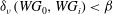


Note that the shaped models are again used in all cases. The second scenario is problematic since it is possible that our particular choice of
 $K_{\infty }$
does not stabilise
$K_{\infty }$
does not stabilise
 $WG_{i}$
. In this case, one option is to alter the system/models in order to reduce the associated uncertainty. Alternatively, the weights
$WG_{i}$
. In this case, one option is to alter the system/models in order to reduce the associated uncertainty. Alternatively, the weights
 $W$
can be changed in order to ensure
$W$
can be changed in order to ensure
 $b(WG_{0},K_{\infty })>{\it\delta}_{{\it\nu}}(WG_{0},WG_{i})$
for all
$b(WG_{0},K_{\infty })>{\it\delta}_{{\it\nu}}(WG_{0},WG_{i})$
for all
 $G_{i}$
. An important note therefore is that the
$G_{i}$
. An important note therefore is that the
 ${\it\nu}$
-gap only provides information regarding the similarity of two models in feedback given the weights
${\it\nu}$
-gap only provides information regarding the similarity of two models in feedback given the weights
 $W$
and is not a measure of the similarity between the two open-loop models in general. In other words, modifying
$W$
and is not a measure of the similarity between the two open-loop models in general. In other words, modifying
 $W$
is likely to have a significant impact on the calculated
$W$
is likely to have a significant impact on the calculated
 ${\it\nu}$
-gap.
${\it\nu}$
-gap.


 Open access