


1. Introduction
Insects take to the air and manoeuvre in three-dimensional space by generating finely tuned aerodynamic force with their flapping wings. While direct flow visualization has played an important role in the field (e.g. Grodnitsky & Morozov Reference Grodnitsky and Morozov1993; Ellington et al. Reference Ellington, van den Berg, Willmott and Thomas1996; Srygley & Thomas Reference Srygley and Thomas2002; Bomphrey et al. Reference Bomphrey, Lawson, Harding, Taylor and Thomas2005; Bomphrey Reference Bomphrey2012), the evaluation of aerodynamic performance through modelling is necessary for comprehensive parameter sweeps and a deeper understanding of flapping-wing aerodynamics.
A blade element model (BEM) with a quasi-steady assumption (that the forces on a flapping wing are equal to those in steady motion at the same instantaneous velocity and attitude of wing blades) has been used as a simple but robust tool for several decades (Weis-Fogh Reference Weis-Fogh1973; Ellington Reference Ellington1984) though it was largely based on steady fixed-wing theory. The BEM has been refined recently by using the lift and drag coefficients of revolving wings (Dickinson, Lehmann & Sane Reference Dickinson, Lehmann and Sane1999; Usherwood & Ellington Reference Usherwood and Ellington2002) and by taking into account rotational circulation and added mass (Dickinson et al. Reference Dickinson, Lehmann and Sane1999; Sane & Dickinson Reference Sane and Dickinson2002). More recently, Berman & Wang (Reference Berman and Wang2007) generalized the BEM for more complicated wing kinematics and utilized the model for optimizing flapping-wing kinematics. Whitney & Wood (Reference Whitney and Wood2010) studied the dynamics of passive wing rotation with a BEM across a range of kinematic parameters and torsional flexibilities, pointing out the importance of torque due to the rotational motion of the wing cross-section. Cheng & Deng (Reference Cheng and Deng2011) expanded the applicability of the BEM to free flight by taking into account the effect of the velocity due to rigid body motion on the local wing attitude and velocity. Nabawy & Crowther (Reference Nabawy and Crowther2014a ,Reference Nabawy and Crowther b ) combined actuator disc and lifting line theories to calculate the induced power factor, and suggested an analytical method for modelling the aerodynamic performance of insect-like flapping wings without the need for experimental data. The quasi-steady model was validated by comparison with CFD predictions by Sun & Du (Reference Sun and Du2003). Kang & Shyy (Reference Kang and Shyy2014) utilized a BEM for constructing a fluid–structure interaction model by combining it with a structural model. These attempts improved the reliability of the BEM and enabled application to various aerodynamic studies such as the dynamics and control of flapping fliers (Hedrick & Daniel Reference Hedrick and Daniel2006; Bergou, Xu & Wang Reference Bergou, Xu and Wang2007; Hedrick, Cheng & Deng Reference Hedrick, Cheng and Deng2009; Kim & Han Reference Kim and Han2014) and the optimization of wing kinematics (Berman & Wang Reference Berman and Wang2007; Zheng, Hedrick & Mittal Reference Zheng, Hedrick and Mittal2013).
However, while its simplicity gives the BEM widespread utility and robustness, its accuracy is still in question. For example, the BEM cannot take into account the three-dimensional effects of the wing tip vortex, which can shift the spanwise position of the centre of pressure. Alternatively, high-fidelity computational simulations based on solving the Navier–Stokes equations (e.g. Sun & Du Reference Sun and Du2003; Liu Reference Liu2009; Liu & Aono Reference Liu and Aono2009; Young et al. Reference Young, Walker, Bomphrey, Taylor and Thomas2009) and dynamically scaled robots (e.g. Dickinson et al. Reference Dickinson, Lehmann and Sane1999) have been used because of their ability to reveal detailed flow structures, time-dependent aerodynamic forces and power requirements with high accuracy and precision. Unfortunately, both high-fidelity modelling and robotics experiments require considerable processing time so it is not practical to directly replace a BEM with either of these approaches.
Here, we propose a novel aerodynamic model, called the CFD-informed quasi-steady model (CIQSM), based on a hybrid of high- and low-fidelity models. To construct the new quasi-steady model, we calculate a set of proportional coefficients that relate wing kinematics to instantaneous aerodynamic force, torque and power by least-squares fitting to high-fidelity CFD results. We use the case of a flapping hawkmoth as an example with which to illustrate the utility of the model.
2. Methods
In this study, a flapping wing is assumed to be rigid, flat and rotating around a pivot with respect to stroke plane as shown in figure 1, so that the wing position, and hence wing velocity and acceleration, can be determined by the given flapping angles. The flapping angles comprise feathering, elevation and positional angles (figure 1). The positional angle is the position of the wing tip in the stroke plane. The elevation angle is the deviation of the spanwise axis from the stroke plane; the wing tip traces a figure-of-eight motion if the elevation angle is appropriately introduced. The feathering angle is the angle of the wing rotation around the spanwise axis on the wing pivot, for directly adjusting the geometric angle of attack. Note that the formulations of the BEM with quasi-steady assumptions are mainly based on Sane & Dickinson (Reference Sane and Dickinson2002) and Berman & Wang (Reference Berman and Wang2007) except for the rotational drag (as detailed below).

Figure 1. (a) Definition of global coordinate system, stroke plane angle, body angle and flapping angles: positional, feathering and elevation angles. (b,c) Definition of the wing-fixed coordinate system viewed with (b) wing planform and (c) cross-section.
2.1. Blade element model of a flapping wing with quasi-steady assumption
The coordinate transformation matrix $\unicode[STIX]{x1D64F}_{w-g}$
that converts from the wing-fixed frame
$\unicode[STIX]{x1D64F}_{w-g}$
that converts from the wing-fixed frame $\left(x,y,z\right)$
to the global frame
$\left(x,y,z\right)$
to the global frame $\left(X,Y,Z\right)$
can be expressed as follows:
$\left(X,Y,Z\right)$
can be expressed as follows:
 $$\begin{eqnarray}\displaystyle & & \displaystyle \hspace{-18.0pt}\unicode[STIX]{x1D64F}_{w-g}=\left(\begin{array}{@{}ccc@{}}1 & 0 & 0\\ 0 & \cos {\it\theta}_{SP} & -\!\sin {\it\theta}_{SP}\\ 0 & \sin {\it\theta}_{SP} & \cos {\it\theta}_{SP}\\ \end{array}\right)\nonumber\\ \displaystyle & & \displaystyle \quad \times \!\left(\begin{array}{@{}ccc@{}}-\!\sin {\it\phi}\cos {\it\alpha}+\cos {\it\phi}\sin {\it\theta}\sin {\it\alpha} & \sin {\it\phi}\sin {\it\alpha}+\cos {\it\phi}\sin {\it\theta}\cos {\it\alpha} & \cos {\it\phi}\cos {\it\theta}\\ \cos {\it\phi}\cos {\it\alpha}+\sin {\it\phi}\sin {\it\theta}\sin {\it\alpha} & -\!\cos {\it\phi}\sin {\it\alpha}+\sin {\it\phi}\sin {\it\theta}\cos {\it\alpha} & \sin {\it\phi}\cos {\it\theta}\\ \cos {\it\theta}\sin {\it\alpha} & \cos {\it\theta}\cos {\it\alpha} & -\!\sin {\it\theta}\\ \end{array}\right)\!\!,\nonumber\\ \displaystyle & & \displaystyle\end{eqnarray}$$
where ${\it\theta}_{SP}$
,
${\it\theta}_{SP}$
, ${\it\phi}$
,
${\it\phi}$
, ${\it\theta}$
and
${\it\theta}$
and ${\it\alpha}$
are the stroke plane angle, the positional angle, the elevation angle and the feathering angle, respectively. The coordinate of a point on the axis of feathering
${\it\alpha}$
are the stroke plane angle, the positional angle, the elevation angle and the feathering angle, respectively. The coordinate of a point on the axis of feathering $\left(0,0,r\right)$
with respect to the global frame, and the angular velocity
$\left(0,0,r\right)$
with respect to the global frame, and the angular velocity $\left(v_{x},v_{y},v_{z}\right)$
and the acceleration
$\left(v_{x},v_{y},v_{z}\right)$
and the acceleration $\left(a_{x},a_{y},a_{z}\right)$
with respect to the wing-fixed frame can be derived as
$\left(a_{x},a_{y},a_{z}\right)$
with respect to the wing-fixed frame can be derived as
 $$\begin{eqnarray}\left(\begin{array}{@{}c@{}}X\\ Y\\ Z\end{array}\right)=\unicode[STIX]{x1D64F}_{w-g}\left(\begin{array}{@{}c@{}}0\\ 0\\ r\end{array}\right)\!,\quad \left(\begin{array}{@{}c@{}}rv_{x}\\ rv_{y}\\ rv_{z}\end{array}\right)=\unicode[STIX]{x1D64F}_{w-g}^{-1}\left(\begin{array}{@{}c@{}}{\dot{X}}\\ {\dot{Y}}\\ {\dot{Z}}\end{array}\right)\!,\quad \left(\begin{array}{@{}c@{}}ra_{x}\\ ra_{y}\\ ra_{z}\end{array}\right)=\unicode[STIX]{x1D64F}_{w-g}^{-1}\left(\begin{array}{@{}c@{}}\ddot{X}\\ \ddot{Y} \\ \ddot{Z}\end{array}\right)\!.\end{eqnarray}$$
Note that $v_{z}$
and
$v_{z}$
and $a_{z}$
are zero in this study due to the rigid wing assumption. In this study, the instantaneous aerodynamic forces
$a_{z}$
are zero in this study due to the rigid wing assumption. In this study, the instantaneous aerodynamic forces $\boldsymbol{F}_{aero}$
generated by the flapping wing are represented as the sum of five quasi-steady forces: translational circulation
$\boldsymbol{F}_{aero}$
generated by the flapping wing are represented as the sum of five quasi-steady forces: translational circulation $\boldsymbol{F}_{tc}$
, translational drag
$\boldsymbol{F}_{tc}$
, translational drag $\boldsymbol{F}_{td}$
, rotational circulation
$\boldsymbol{F}_{td}$
, rotational circulation $\boldsymbol{F}_{rc}$
, force due to added mass
$\boldsymbol{F}_{rc}$
, force due to added mass $\boldsymbol{F}_{am}$
and rotational drag
$\boldsymbol{F}_{am}$
and rotational drag $\boldsymbol{F}_{rd}$
:
$\boldsymbol{F}_{rd}$
:
 $$\begin{eqnarray}\boldsymbol{F}_{aero}=\boldsymbol{F}_{tc}+\boldsymbol{F}_{td}+\boldsymbol{F}_{rc}+\boldsymbol{F}_{am}+\boldsymbol{F}_{rd}.\end{eqnarray}$$
The rotational drag is the drag force due to wing rotation around the spanwise axis, and has been neglected in most previous studies. However, it must be taken into account in order to calculate three-dimensional forces and power accurately as discussed in the study by Whitney & Wood (Reference Whitney and Wood2010), in which they pointed out that rotational drag is crucial to accurately predicting the dynamic passive rotation of flapping wings. The quasi-steady forces based on the BEM can be given as follows (Sane & Dickinson Reference Sane and Dickinson2002; Berman & Wang Reference Berman and Wang2007; Whitney & Wood Reference Whitney and Wood2010):
 $$\begin{eqnarray}\displaystyle & \displaystyle F_{tc}=\frac{1}{2}{\it\rho}\int _{0}^{R}r^{2}c_{l}\,\text{d}r~C_{L}(\text{AoA})|\boldsymbol{v}|^{2}, & \displaystyle\end{eqnarray}$$
 $$\begin{eqnarray}\displaystyle & \displaystyle F_{td}=\frac{1}{2}{\it\rho}\int _{0}^{R}r^{2}c_{l}\,\text{d}r~C_{D}(\text{AoA})|\boldsymbol{v}|^{2}, & \displaystyle\end{eqnarray}$$
 $$\begin{eqnarray}\displaystyle & \displaystyle F_{rc}={\it\rho}\int _{0}^{R}rc_{l}^{2}\,\text{d}r~C_{RL}\dot{{\it\alpha}}|\boldsymbol{v}|, & \displaystyle\end{eqnarray}$$
 $$\begin{eqnarray}\displaystyle & \displaystyle F_{am}={\it\rho}\frac{{\rm\pi}}{4}\int _{0}^{R}rc_{l}^{2}\,\text{d}r~(a_{y}+\dot{{\it\alpha}}v_{x})+{\it\rho}\frac{{\rm\pi}}{16}\int _{0}^{R}c_{l}^{3}\,\text{d}r~\ddot{{\it\alpha}}, & \displaystyle\end{eqnarray}$$
 $$\begin{eqnarray}\displaystyle & \displaystyle F_{rd}=\frac{1}{2}{\it\rho}\int _{c_{te}}^{c_{le}}r_{l}c^{2}\,\text{d}c~C_{RD}\dot{{\it\alpha}}|\dot{{\it\alpha}}|, & \displaystyle\end{eqnarray}$$ ${\it\rho}$
is the density of air,
${\it\rho}$
is the density of air, $R$
is the wing length,
$R$
is the wing length, $c_{l}$
and
$c_{l}$
and $r_{l}$
are the local chordwise and spanwise lengths respectively,
$r_{l}$
are the local chordwise and spanwise lengths respectively, $|\boldsymbol{v}|$
is the absolute angular velocity given by
$|\boldsymbol{v}|$
is the absolute angular velocity given by $\sqrt{v_{x}^{2}+v_{y}^{2}}$
, AoA is the geometric angle of attack, and
$\sqrt{v_{x}^{2}+v_{y}^{2}}$
, AoA is the geometric angle of attack, and $C_{L}$
,
$C_{L}$
, $C_{D}$
,
$C_{D}$
, $C_{RL}$
and
$C_{RL}$
and $C_{RD}$
are the lift, drag, rotational lift and rotational drag coefficients, respectively.
$C_{RD}$
are the lift, drag, rotational lift and rotational drag coefficients, respectively. $C_{L}$
and
$C_{L}$
and $C_{D}$
are functions of AoA, and can be, for instance, expressed as follows:
$C_{D}$
are functions of AoA, and can be, for instance, expressed as follows:  $$\begin{eqnarray}\displaystyle & \displaystyle C_{L}=C_{L1}\left(\text{AoA}^{3}-\frac{{\rm\pi}}{2}\text{AoA}^{2}\right)+C_{L2}\left(\text{AoA}^{2}-\frac{{\rm\pi}}{2}\text{AoA}\right), & \displaystyle\end{eqnarray}$$
 $$\begin{eqnarray}\displaystyle & \displaystyle C_{D}=C_{Dmin}\cos ^{2}\text{AoA}+C_{Dmax}\sin ^{2}\text{AoA}. & \displaystyle\end{eqnarray}$$ $C_{L}$
has been expressed as a sinusoidal function (e.g.
$C_{L}$
has been expressed as a sinusoidal function (e.g. $C_{L}=\sin \left(2\text{AoA}\right)$
), but here we employ more complicated forms of the
$C_{L}=\sin \left(2\text{AoA}\right)$
), but here we employ more complicated forms of the $C_{L}$
–AoA curve as depicted in figure 2.
$C_{L}$
–AoA curve as depicted in figure 2.

Figure 2. Parameterized lift-force coefficients as a function of geometric angle of attack.
2.2. CFD-informed quasi-steady model
The quasi-steady forces in (2.4) can then be rewritten by breaking up each quasi-steady force into the kinematics-related terms and the terms relating to the density of fluid, the force coefficients and wing shape for translational circulation ( $I_{tc1}$
,
$I_{tc1}$
, $I_{tc2}$
), translational drag (
$I_{tc2}$
), translational drag ( $I_{td1}$
,
$I_{td1}$
, $I_{td2}$
), rotational circulation (
$I_{td2}$
), rotational circulation ( $I_{rc}$
), force due to added mass (
$I_{rc}$
), force due to added mass ( $I_{am1}$
,
$I_{am1}$
, $I_{am2}$
,
$I_{am2}$
, $I_{am3}$
) and rotational drag (
$I_{am3}$
) and rotational drag ( $I_{rd}$
) as follows:
$I_{rd}$
) as follows:
 $$\begin{eqnarray}\displaystyle & \displaystyle F_{tc}=I_{tc1}\left(\text{AoA}^{3}-\frac{{\rm\pi}}{2}\text{AoA}^{2}\right)|\boldsymbol{v}|^{2}+I_{tc2}\left(\text{AoA}^{2}-\frac{{\rm\pi}}{2}\text{AoA}\right)|\boldsymbol{v}|^{2}, & \displaystyle\end{eqnarray}$$
 $$\begin{eqnarray}\displaystyle & \displaystyle F_{td}=I_{td1}\cos ^{2}\left(\text{AoA}\right)|\boldsymbol{v}|^{2}+I_{td2}\sin ^{2}\left(\text{AoA}\right)|\boldsymbol{v}|^{2}, & \displaystyle\end{eqnarray}$$
 $$\begin{eqnarray}\displaystyle & \displaystyle F_{rc}=I_{rc}\dot{{\it\alpha}}|\boldsymbol{v}|, & \displaystyle\end{eqnarray}$$
 $$\begin{eqnarray}\displaystyle & \displaystyle F_{am}=I_{am1}a_{y}+I_{am2}\dot{{\it\alpha}}v_{x}+I_{am3}\ddot{{\it\alpha}}, & \displaystyle\end{eqnarray}$$
 $$\begin{eqnarray}\displaystyle & \displaystyle F_{rd}=I_{rd}\dot{{\it\alpha}}|\dot{{\it\alpha}}|. & \displaystyle\end{eqnarray}$$
 $$\begin{eqnarray}\left(\begin{array}{@{}c@{}}F_{X}\\ F_{Y}\\ F_{Z}\end{array}\right)=\unicode[STIX]{x1D64F}_{w-g}\left(\begin{array}{@{}c@{}}F_{x}\\ F_{y}\\ 0\end{array}\right)=\boldsymbol{k}_{f}\left({\it\phi},{\it\theta},{\it\alpha}\right)\boldsymbol{\cdot }\unicode[STIX]{x1D644}_{f},\end{eqnarray}$$
where $\boldsymbol{k}_{f}$
represents wing kinematics parameters in (2.6) with respect to the global coordinate system, and
$\boldsymbol{k}_{f}$
represents wing kinematics parameters in (2.6) with respect to the global coordinate system, and
 $$\begin{eqnarray}\begin{array}{@{}ccccccccc@{}}\unicode[STIX]{x1D644}_{f}= [I_{tc1} & I_{tc2} & I_{td1} & I_{td2} & I_{rc} & I_{am1} & I_{am2} & I_{am3} & I_{rd} ]^{\text{T}}.\end{array}\end{eqnarray}$$
This relationship suggests that, under a quasi-steady assumption, the aerodynamic force is proportional to nine variables defined by the instantaneous angular velocity and acceleration of the wing and the wing’s attitude. The proportional coefficients $\unicode[STIX]{x1D644}_{f}$
are related to fluid density, force coefficients and wing shape, and are conventionally derived by a BEM that assumes a wing to be a series of blades so that one can calculate the shape coefficients analytically or numerically as in (2.4). However, we are also able to obtain these coefficients by fitting the instantaneous aerodynamic forces from a computational, or robotic, high-fidelity model. If we assume that
$\unicode[STIX]{x1D644}_{f}$
are related to fluid density, force coefficients and wing shape, and are conventionally derived by a BEM that assumes a wing to be a series of blades so that one can calculate the shape coefficients analytically or numerically as in (2.4). However, we are also able to obtain these coefficients by fitting the instantaneous aerodynamic forces from a computational, or robotic, high-fidelity model. If we assume that $\boldsymbol{F}_{CFD}$
represents the instantaneous aerodynamic forces by some high-fidelity model, the sum of the squared residuals,
$\boldsymbol{F}_{CFD}$
represents the instantaneous aerodynamic forces by some high-fidelity model, the sum of the squared residuals,
 $$\begin{eqnarray}{\it\epsilon}_{r}=\left(\boldsymbol{F}_{CFD}-\boldsymbol{k}_{f}\boldsymbol{\cdot }\unicode[STIX]{x1D644}_{f}\right)^{\text{T}}\left(\boldsymbol{F}_{CFD}-\boldsymbol{k}_{f}\boldsymbol{\cdot }\unicode[STIX]{x1D644}_{f}\right)=\mathop{\sum }_{i}\left(F_{CFD,i}-\boldsymbol{k}_{f,i}\boldsymbol{\cdot }\unicode[STIX]{x1D644}_{f}\right)^{2},\end{eqnarray}$$
is minimized when
 $$\begin{eqnarray}\unicode[STIX]{x1D644}_{f}=\left(\boldsymbol{k}_{f}\boldsymbol{k}_{f}^{T}\right)^{-1}\boldsymbol{k}_{f}\boldsymbol{F}_{CFD}^{T}.\end{eqnarray}$$
Obviously, this model is capable of dealing with arbitrary wing kinematics once it is established. The $\boldsymbol{k}_{f,i}$
and
$\boldsymbol{k}_{f,i}$
and $F_{CFD,i}$
are both instantaneous values, and therefore even a single simulation can give a lot of data points if the wing velocity and acceleration are changed dynamically. In order to keep the amount of information from each CFD result constant, the forces and torques are interpolated so as to give 1000 points for each wing beat cycle rather than the variable number of time steps that arise as a consequence of varying the mean wing tip velocity. When multiple CFD results are used for fitting, the
$F_{CFD,i}$
are both instantaneous values, and therefore even a single simulation can give a lot of data points if the wing velocity and acceleration are changed dynamically. In order to keep the amount of information from each CFD result constant, the forces and torques are interpolated so as to give 1000 points for each wing beat cycle rather than the variable number of time steps that arise as a consequence of varying the mean wing tip velocity. When multiple CFD results are used for fitting, the $\boldsymbol{k}_{f}$
and
$\boldsymbol{k}_{f}$
and $\boldsymbol{F}_{CFD}$
for each CFD result are simply concatenated. In order to avoid overestimating the least-squares errors from a single case, the forces or torques in each case are normalized by
$\boldsymbol{F}_{CFD}$
for each CFD result are simply concatenated. In order to avoid overestimating the least-squares errors from a single case, the forces or torques in each case are normalized by ${\it\rho}U_{ref}^{2}c_{m}^{2}$
and
${\it\rho}U_{ref}^{2}c_{m}^{2}$
and ${\it\rho}U_{ref}^{2}c_{m}^{3}$
, respectively, where
${\it\rho}U_{ref}^{2}c_{m}^{3}$
, respectively, where $U_{ref}$
is the mean wing tip velocity and
$U_{ref}$
is the mean wing tip velocity and $c_{m}$
is the mean chord length.
$c_{m}$
is the mean chord length.

Figure 3. Definition of translational and rotational torque.
Aerodynamic power can be calculated as the dot product of aerodynamic torque and angular velocity. The aerodynamic torque in BEM is normally calculated by summing the products of the blade force based on the force coefficients and their distance from wing base. However, the quasi-steady assumption results in a quadratic distribution of the force per unit area, and therefore underestimates the three-dimensional effects of the wing tip vortex. In order to take into account such effects, we chose to fit the shape-dependent coefficients for aerodynamic torque separately, in a similar way to that for estimating aerodynamic force, rather than directly using $\unicode[STIX]{x1D644}_{f}$
for forces. As the forces on the wing should induce both translational and rotational torques, the number of coefficients is simply doubled. The locations where the quasi-steady forces act are uncertain at the outset but defined in figure 3. The torque with respect to the wing-fixed frame
$\unicode[STIX]{x1D644}_{f}$
for forces. As the forces on the wing should induce both translational and rotational torques, the number of coefficients is simply doubled. The locations where the quasi-steady forces act are uncertain at the outset but defined in figure 3. The torque with respect to the wing-fixed frame $\left(T_{x},T_{y},T_{z}\right)$
can be expressed as follows:
$\left(T_{x},T_{y},T_{z}\right)$
can be expressed as follows:
 $$\begin{eqnarray}\left(\begin{array}{@{}c@{}}T_{x}\\ T_{y}\\ T_{z}\end{array}\right)=\left(\begin{array}{@{}c@{}}-r_{p}F_{y}\\ r_{p}F_{x}\\ c_{p}F_{y}\end{array}\right)\!,\end{eqnarray}$$
where $r_{p}$
and
$r_{p}$
and $c_{p}$
are the spanwise and chordwise locations where the aerodynamic force acts, respectively. Accordingly, aerodynamic torques with respect to the global frame
$c_{p}$
are the spanwise and chordwise locations where the aerodynamic force acts, respectively. Accordingly, aerodynamic torques with respect to the global frame $\left(T_{X},T_{Y},T_{Z}\right)$
can be written in matrix form as follows:
$\left(T_{X},T_{Y},T_{Z}\right)$
can be written in matrix form as follows:
 $$\begin{eqnarray}\left(\begin{array}{@{}c@{}}T_{X}\\ T_{Y}\\ T_{Z}\end{array}\right)=\unicode[STIX]{x1D64F}_{w-g}\left(\begin{array}{@{}ccc@{}}0 & -1 & 0\\ 1 & 0 & 0\\ 0 & 0 & 0\\ \end{array}\right)\boldsymbol{k}_{fl}\boldsymbol{\cdot }\unicode[STIX]{x1D644}_{f}r_{p}+\unicode[STIX]{x1D64F}_{w-g}\left(\begin{array}{@{}ccc@{}}0 & 0 & 0\\ 0 & 0 & 0\\ 0 & 1 & 0\\ \end{array}\right)\boldsymbol{k}_{fl}\boldsymbol{\cdot }\unicode[STIX]{x1D644}_{f}c_{p},\end{eqnarray}$$
where $\boldsymbol{k}_{fl}$
stands for the
$\boldsymbol{k}_{fl}$
stands for the $\boldsymbol{k}_{f}$
with respect to wing-fixed frame so that
$\boldsymbol{k}_{f}$
with respect to wing-fixed frame so that $\boldsymbol{k}_{f}=\unicode[STIX]{x1D64F}_{w-g}\boldsymbol{k}_{fl}$
. By defining the kinematics parameter for torque
$\boldsymbol{k}_{f}=\unicode[STIX]{x1D64F}_{w-g}\boldsymbol{k}_{fl}$
. By defining the kinematics parameter for torque $\boldsymbol{k}_{t}$
and shape-dependent parameter
$\boldsymbol{k}_{t}$
and shape-dependent parameter $\unicode[STIX]{x1D644}_{t}$
, (2.12) can be rewritten as follows:
$\unicode[STIX]{x1D644}_{t}$
, (2.12) can be rewritten as follows:
 $$\begin{eqnarray}\displaystyle \left(\begin{array}{@{}c@{}}T_{X}\\ T_{Y}\\ T_{Z}\end{array}\right)=\boldsymbol{k}_{tt}\boldsymbol{\cdot }\unicode[STIX]{x1D644}_{tt}+\boldsymbol{k}_{rt}\boldsymbol{\cdot }\unicode[STIX]{x1D644}_{rt}=\boldsymbol{k}_{t}\boldsymbol{\cdot }\unicode[STIX]{x1D644}_{t}, & & \displaystyle\end{eqnarray}$$
where the subscripts $tt$
and
$tt$
and $rt$
represent translational torque and rotational torque, respectively. Once the instantaneous aerodynamic torques are known, we can fit
$rt$
represent translational torque and rotational torque, respectively. Once the instantaneous aerodynamic torques are known, we can fit $\unicode[STIX]{x1D644}_{t}$
in the same way as for aerodynamic force, as shown in (2.10). By using the aerodynamic torque, the aerodynamic power is calculated as the product of the torques and angular velocities as follows:
$\unicode[STIX]{x1D644}_{t}$
in the same way as for aerodynamic force, as shown in (2.10). By using the aerodynamic torque, the aerodynamic power is calculated as the product of the torques and angular velocities as follows:
 $$\begin{eqnarray}\displaystyle P & = & \displaystyle T_{x}\left(\dot{{\it\phi}}\cos {\it\theta}\sin {\it\alpha}+\dot{{\it\theta}}\cos {\it\alpha}\right)+T_{y}\left(\dot{{\it\phi}}\cos {\it\theta}\cos {\it\alpha}-\dot{{\it\theta}}\sin {\it\alpha}\right)\nonumber\\ \displaystyle & & \displaystyle +\,T_{z}\left(\dot{{\it\alpha}}-\dot{{\it\phi}}\sin {\it\theta}\right)\!.\end{eqnarray}$$
2.3. CFD model of a hovering hawkmoth
A high-fidelity simulation is essential for informing the quasi-steady model. This study employs a versatile CFD-based dynamic flight simulator (Liu Reference Liu2009) that easily integrates the modelling of realistic wing–body morphology, realistic wing–body kinematics and unsteady aerodynamics in insect flight. Details can be found in previous publications (Liu Reference Liu2009; Nakata & Liu Reference Nakata and Liu2012).
To validate the CIQSM, we have used a model of a hovering hawkmoth. The morphology and kinematic patterns are constructed based on measurements from previous studies (figure 4 a,b; Willmott & Ellington Reference Willmott and Ellington1997; Aono & Liu Reference Aono and Liu2006). Each wing is modelled separately as a single computational grid, and subsequently merged with a global body grid. The parameters regarding wing shape, wing kinematics, Reynolds number, reduced frequency (based on mean wing tip velocity) and computational conditions are summarized in table 1.

Figure 4. Computational model of a hovering hawkmoth. (a) Wing–body morphological model for CFD and wing models for BEM with chordwise and spanwise blades, and (b) kinematic models of a hovering hawkmoth. (c) Wing tip trajectories and wing attitude of a realistic (black) and a modified (purple) wing kinematics. (d–h) Modified flapping angles.
Table 1. Computational parameters.

The simulations are carried out with a range of wing kinematics that have been modified from published data for a hovering hawkmoth (figure 4 b; Willmott & Ellington Reference Willmott and Ellington1997; Aono & Liu Reference Aono and Liu2006) in order to construct the quasi-steady model and estimate its accuracy. As shown in figure 4, the range of wing kinematics is created by varying: (i) duration of the stroke reversal (or duration of constant angle of attack; figure 4 d), (ii) phase of feathering angle with respect to positional angle (10 % delayed to 10 % advanced; figure 4 e), (iii) amplitude of feathering angle (or geometric angle of attack; 80 % to 120 % of realistic; figure 4 f), (iv) wing beat amplitude (80–120 %; figure 4 g), (v) wing beat frequency (80–120 %), (vi) amplitude and waveform of elevation angle (0–200 %; figure 4 h), so that the wing tips trace a ‘parabola’ trajectory or ‘figure-of-eight’ trajectory (figure 4 c).
2.4. Validation
The error of the CIQSM is evaluated by subsampling the available CFD results so that a probability distribution of the error can be estimated. First, the quasi-steady model is constructed using a random subsample of the available CFD data. For validation, the quasi-steady model only evaluates the aerodynamic performance of kinematic patterns that are not used for its construction. Quasi-steady predictions are then compared with the CFD results for same wing kinematics so that we can estimate the accuracy of the model with various CFD-based input data for quasi-steady model construction. The performance of the model, or error, is then evaluated by using two indices: the absolute mean error ${\it\epsilon}$
and Pearson correlation coefficient (PCC)
${\it\epsilon}$
and Pearson correlation coefficient (PCC) ${\it\sigma}$
,
${\it\sigma}$
,
 $$\begin{eqnarray}{\it\epsilon}=\frac{1}{k}\mathop{\sum }_{i=1}^{k}\left|\frac{\overline{f_{i}}-\overline{f_{i}^{CFD}}}{\overline{f_{i}^{CFD}}}\right|,\quad {\it\sigma}=\frac{\text{cov}(f,f^{CFD})}{\text{std}(f)\,\text{std}(f^{CFD})},\end{eqnarray}$$
where $k$
is the number of cases for prediction,
$k$
is the number of cases for prediction, $f_{i}$
and
$f_{i}$
and $f_{i}^{CFD}$
represent the quasi-steady and CFD-based predictions, and cov and std represent the covariance and standard deviation, respectively. For the PCC,
$f_{i}^{CFD}$
represent the quasi-steady and CFD-based predictions, and cov and std represent the covariance and standard deviation, respectively. For the PCC, $f$
can be either the time series of the prediction from one case or the mean values from multiple cases.
$f$
can be either the time series of the prediction from one case or the mean values from multiple cases.
For the sake of comparison, we have also calculated the aerodynamic forces and power with BEM. The aerodynamic forces are given by (2.4), in which $C_{L}$
and
$C_{L}$
and $C_{D}$
are taken from Usherwood & Ellington (Reference Usherwood and Ellington2002). The formulation of rotational circulation and the force due to added mass are based on those by Sane & Dickinson (Reference Sane and Dickinson2002). The coefficient of rotational circulation is given as
$C_{D}$
are taken from Usherwood & Ellington (Reference Usherwood and Ellington2002). The formulation of rotational circulation and the force due to added mass are based on those by Sane & Dickinson (Reference Sane and Dickinson2002). The coefficient of rotational circulation is given as $C_{RL}=0.55$
(Zheng et al.
Reference Zheng, Hedrick and Mittal2013). The rotational drag is the drag due to rotation around the spanwise axis, and hence calculated by assuming spanwise blades rather than chordwise blades for the BEM (see figure 4
a). As the rotational drag is the drag at 90° angle of attack, the maximum value of
$C_{RL}=0.55$
(Zheng et al.
Reference Zheng, Hedrick and Mittal2013). The rotational drag is the drag due to rotation around the spanwise axis, and hence calculated by assuming spanwise blades rather than chordwise blades for the BEM (see figure 4
a). As the rotational drag is the drag at 90° angle of attack, the maximum value of $C_{D}$
measured by Usherwood & Ellington (Reference Usherwood and Ellington2002) is employed for the
$C_{D}$
measured by Usherwood & Ellington (Reference Usherwood and Ellington2002) is employed for the $C_{RD}$
. The translational torque due to the translational lift and drag, the rotational lift and the force due to added mass are calculated by summing the products of the forces on each chordwise blade and the distance between the chordwise blade and the pivot. The chordwise location of the centre of pressure that depends upon angle of attack is taken from Dickson, Straw & Dickinson (Reference Dickson, Straw and Dickinson2008). The contribution of translational lift and drag to the rotational torque is calculated by using the distance between the centre of pressure (Dickson et al.
Reference Dickson, Straw and Dickinson2008) and the feathering axis. The force due to added mass is assumed to be acting on the centre of the chordwise blade. The rotational drag is assumed to be acting on the middle of each spanwise blade, assuming
$C_{RD}$
. The translational torque due to the translational lift and drag, the rotational lift and the force due to added mass are calculated by summing the products of the forces on each chordwise blade and the distance between the chordwise blade and the pivot. The chordwise location of the centre of pressure that depends upon angle of attack is taken from Dickson, Straw & Dickinson (Reference Dickson, Straw and Dickinson2008). The contribution of translational lift and drag to the rotational torque is calculated by using the distance between the centre of pressure (Dickson et al.
Reference Dickson, Straw and Dickinson2008) and the feathering axis. The force due to added mass is assumed to be acting on the centre of the chordwise blade. The rotational drag is assumed to be acting on the middle of each spanwise blade, assuming $\text{AoA}=90^{\circ }$
, in order to calculate the translational and rotational torques.
$\text{AoA}=90^{\circ }$
, in order to calculate the translational and rotational torques.
3. Results and discussion
3.1. Comparison between conventional BEM and CFD
Time courses of simulated aerodynamic forces and power generated by a single flapping wing with realistic wing kinematics are illustrated in figure 5. These CFD results showed that considerable three-dimensional forces are produced during the translational phase of both downstroke and upstroke due to the attached leading edge vortex (LEV; Maxworthy Reference Maxworthy1979; Ellington et al.
Reference Ellington, van den Berg, Willmott and Thomas1996; Bomphrey et al.
Reference Bomphrey, Lawson, Harding, Taylor and Thomas2005; Aono & Liu Reference Aono and Liu2006). A large aerodynamic power is required to generate such high aerodynamic forces (figure 5
c). More details on the force generation, the power requirement and the corresponding flow structure are discussed in Aono & Liu (Reference Aono and Liu2006) and Lua et al. (Reference Lua, Lai, Lim and Yep2010). When considering the wing-fixed frame of reference, the chordwise and spanwise aerodynamic forces ( $F_{x}$
and
$F_{x}$
and $F_{z}$
) are negligibly small in comparison with the normal force,
$F_{z}$
) are negligibly small in comparison with the normal force, $F_{y}$
(figure 5
b). In fact, the absolute means of the chordwise and spanwise forces are 1.3 % and 0.3 % of the normal force, respectively. This is favourable for the BEM because it cannot predict spanwise forces.
$F_{y}$
(figure 5
b). In fact, the absolute means of the chordwise and spanwise forces are 1.3 % and 0.3 % of the normal force, respectively. This is favourable for the BEM because it cannot predict spanwise forces.

Figure 5. Aerodynamic forces and power predicted by CFD with realistic wing kinematics. (a–c) Time courses of aerodynamic force with respect to (a) the global coordinate system and (b) the wing-fixed coordinate system, and (c) aerodynamic power. The shaded area corresponds to the downstroke.
The mean vertical aerodynamic force and aerodynamic power results from the CFD and BEM methods are summarized in figure 6 for the realistic as well as modified wing kinematic patterns. By tuning the wing kinematics, both force and power range over an order of magnitude from 3.4 to 18.6 mN and 9.3 to 120 mW, respectively. The BEM predictions are in reasonable agreement with those from CFD. The PCC of the mean force and power are 0.962 and 0.955, respectively, which means good correlation between the predictions by the BEM and the CFD. The mean errors are about 10.1 % and 9.04 %, respectively. As mentioned above, the error in the conventional BEM is thought to be because the BEM inherently overlooks the effect of downwash on the angle of attack and the effect of the wing tip vortex, which affects the spanwise position of the centre of the pressure.

Figure 6. Comparisons of (a) mean vertical forces and (b) mean aerodynamic powers predicted by CFD (horizontal axis) and the BEM (vertical axis).
3.2. Construction and general applicability of the CFD-informed quasi-steady model
Once the aerodynamic force and power for varying wing kinematics have been used to parameterize the quasi-steady model, the CIQSM can be validated by appraising the error of the mean values and the PCC of instantaneous values compared with the CFD result that is used for constructing the quasi-steady model. With these comparisons, the general applicability of the quasi-steady model to flapping-wing aerodynamics can be discussed because this is the best fit of the quasi-steady model to high-fidelity simulation. At this point, we can get an upper limit on the performance of the quasi-steady model. The time series of high-fidelity CFD and CIQSM aerodynamic forces and power are shown in figure 7. Unsurprisingly, the quasi-steady force and power are in close agreement with the CFD model in this case, which suggests that the aerodynamic force generation and power consumption by the standard wing shape and the realistic kinematics can be explained in a quasi-steady manner. The PCCs of instantaneous vertical force and power are 0.97 and 0.98, and the errors of mean force and power are 0.38 % and 1.98 %, respectively.

Figure 7. Comparison of (a) aerodynamic vertical force and (b) aerodynamic power simulated by CFD (dashed black) and CIQSM (solid black). Coloured components sum to solid black lines.

Figure 8. Time courses of (a,d) aerodynamic forces and (b,c) flow structure at several time instants A–E by (a,b) realistic kinematics and (c,d) 10 % delayed rotation. While the LEV highlighted by the red line is kept attached on the wing with realistic wing kinematics through the downstroke, the LEV is detached at early downstroke (B) by 10 % delayed rotation. Vortex wake is identified by iso-surfaces at $Q=0.5$
, coloured by spanwise vorticity.
$Q=0.5$
, coloured by spanwise vorticity.
Once the quasi-steady model is constructed, the vertical force and power can be decomposed into the contributions of the translational circulation, the translational drag, the rotational circulation, the rotational drag and the force due to added mass as shown in figure 7. Downstroke and upstroke asymmetry in vertical force is principally due to the increase in translational drag during downstroke because of the inclined stroke plane. The contribution of translational drag to the vertical force is reduced during the upstroke because of the lower angle of attack. High acceleration and rapid rotation during stroke reversal lead to a sharp rise in rotational drag and also the force due to added mass. Hence, there is a second peak in vertical forces during both upstroke and downstroke. The power due to translational drag accounts for the majority of the power consumption but other components, such as rotational drag, also have a notable effect. Note that the remaining discrepancy between the results can be attributed to wing–wake interaction such as wake capture (Dickinson et al. Reference Dickinson, Lehmann and Sane1999). Wake capture changes the angle of attack and can shift the phase of the force or skew it.
The CIQSMs from the modified wing kinematics also compare satisfactorily with the CFD results. The mean errors of vertical force and power are 0.78 % and 1.56 % while the mean PCCs of instantaneous vertical forces and powers are 0.97 and 0.99. The kinematic conditions under which the model performs least well occur when there is a 10 % delay in wing rotation when the error and the PCC of the vertical force were 2.84 % and 0.93, respectively. The time series of vertical forces by CFD and quasi-steady fitting with the realistic wing kinematics (upper) and 10 % delayed rotation (lower) are given in figure 8(a,d). As can be seen, while the CIQSM force closely matches the CFD simulation under realistic wing kinematics, the two methods deviate from one another when wing rotation is delayed; the deviation is particularly prominent during the downstroke. In order to understand the flow physics that causes this error, the vortex structure is visualized at several intervals during the downstroke (A–E in figure 8
a,d). For clarity, we have used the $Q$
-criterion for vortex identification in figure 8(b,c) (
$Q$
-criterion for vortex identification in figure 8(b,c) ( $Q=0.5$
; Jeong & Hussain Reference Jeong and Hussain1995). With the realistic wing kinematics, at early downstroke and as the wing completes pronation, the LEV (red line) and the trailing edge vortex (TEV, blue line) grow in size from wing base towards the wing tip (A). The TEV subsequently detaches from the wing, forming a starting vortex that connects to the LEV through the wing tip vortex (B–C). Even though the LEV becomes unstable near the wing tip at late downstroke, the LEV remains attached through the downstroke. In contrast, when rotation is delayed, the high angle of attack at early downstroke causes the LEV to detach much earlier, which in turn causes a reduction in the peak forces of 60 % (B). The TEV is subsequently detached and a second LEV grows rapidly, which increases the vertical force as the wing approaches time step D in the CFD results, but the force decreases again after time step E due to the wing’s deceleration. This complex vortex shedding with delayed rotation is also observed in the previous study by Zheng et al. (Reference Zheng, Hedrick and Mittal2013), in which they suggested that phenomena associated with the timing of rotation limit the BEM accuracy. In this study, it is found that, even if the coefficients are fully calculated by the fitting to the CFD results, the change in aerodynamic force and power caused by vortex breakdown and detachment cannot be modelled accurately because the quasi-steady model implicitly assumes that the variation in aerodynamic force is caused by the instantaneous wing velocity and acceleration. However, it should be emphasized that the effect of such vortex detachment can be incorporated into the quasi-steady model by fitting high-fidelity simulations or robotic model data. This implies that the accuracy of the quasi-steady model can be higher if the number of input cases, or, in other words, the amount of information regarding the relationship between wing velocity and aerodynamic force, is increased.
$Q=0.5$
; Jeong & Hussain Reference Jeong and Hussain1995). With the realistic wing kinematics, at early downstroke and as the wing completes pronation, the LEV (red line) and the trailing edge vortex (TEV, blue line) grow in size from wing base towards the wing tip (A). The TEV subsequently detaches from the wing, forming a starting vortex that connects to the LEV through the wing tip vortex (B–C). Even though the LEV becomes unstable near the wing tip at late downstroke, the LEV remains attached through the downstroke. In contrast, when rotation is delayed, the high angle of attack at early downstroke causes the LEV to detach much earlier, which in turn causes a reduction in the peak forces of 60 % (B). The TEV is subsequently detached and a second LEV grows rapidly, which increases the vertical force as the wing approaches time step D in the CFD results, but the force decreases again after time step E due to the wing’s deceleration. This complex vortex shedding with delayed rotation is also observed in the previous study by Zheng et al. (Reference Zheng, Hedrick and Mittal2013), in which they suggested that phenomena associated with the timing of rotation limit the BEM accuracy. In this study, it is found that, even if the coefficients are fully calculated by the fitting to the CFD results, the change in aerodynamic force and power caused by vortex breakdown and detachment cannot be modelled accurately because the quasi-steady model implicitly assumes that the variation in aerodynamic force is caused by the instantaneous wing velocity and acceleration. However, it should be emphasized that the effect of such vortex detachment can be incorporated into the quasi-steady model by fitting high-fidelity simulations or robotic model data. This implies that the accuracy of the quasi-steady model can be higher if the number of input cases, or, in other words, the amount of information regarding the relationship between wing velocity and aerodynamic force, is increased.

Figure 9. Error estimation of the quasi-steady predictions illustrated by the probability distributions of the estimated error and PCC of (a,b) mean vertical aerodynamic force and (c,d) mean aerodynamic power by the CIQSM. (a,c) Mean error of the CIQSM predictions compared with high-fidelity CFD simulations. (b,d) PCC of mean aerodynamic vertical forces or power between CFD and quasi-steady predictions. Vertical black lines show the prediction of a BEM, which is significantly less accurate in all cases.
3.3. Accuracy of force and power predictions by the CFD-informed quasi-steady model
To validate the CIQSM, we used between 5 and 23 of the high-fidelity CFD test cases (out of a total of 29 cases; figure 4) as the number of input cases for informing the quasi-steady model. For each number of input cases, $10^{5}$
combinations of input cases are randomly sampled for the test. The histograms in figure 9 show the probability distribution of the mean errors and PCCs between CFD and CIQSM predictions of the mean vertical force and power. The errors and PCCs of predictions from a conventional BEM are also shown for comparison (vertical lines). As the number of input cases becomes larger, there is a clear trend showing a decreasing median of errors and an increasing median of PCCs. As mentioned above, this is due to the increase in information for the construction of the quasi-steady model. The mean vertical forces and power predicted by the CIQSM with 23 input cases and CFD are summarized in figure 10. The predictions are quite consistent and the standard deviations are smaller than the size of the plotted data points in figure 10. Most of the predictions of CIQSM are very close to the values obtained using CFD. The highest errors in vertical force and power predictions occur when there is 10 % delay and an advance in rotation (triangle and square plots in figure 10). The slight increase in the probability of high error and low PCC when using a large number of input cases occurs when the test cases include such extreme kinematic cases, i.e. 10 % delayed rotation for force, and 5 and 10 % delayed and 10 % advanced rotation for power. The quasi-steady prediction of 10 % delayed rotation is less accurate because of the vortex detachment in early downstroke as shown above. The quasi-steady model also fails to predict well the performance of kinematic patterns exhibiting advanced rotation because of a strong wake capture effect (Dickinson et al.
Reference Dickinson, Lehmann and Sane1999). However, the mean errors of lift and power are likely to be less than that of a BEM even if such risky cases are included.
$10^{5}$
combinations of input cases are randomly sampled for the test. The histograms in figure 9 show the probability distribution of the mean errors and PCCs between CFD and CIQSM predictions of the mean vertical force and power. The errors and PCCs of predictions from a conventional BEM are also shown for comparison (vertical lines). As the number of input cases becomes larger, there is a clear trend showing a decreasing median of errors and an increasing median of PCCs. As mentioned above, this is due to the increase in information for the construction of the quasi-steady model. The mean vertical forces and power predicted by the CIQSM with 23 input cases and CFD are summarized in figure 10. The predictions are quite consistent and the standard deviations are smaller than the size of the plotted data points in figure 10. Most of the predictions of CIQSM are very close to the values obtained using CFD. The highest errors in vertical force and power predictions occur when there is 10 % delay and an advance in rotation (triangle and square plots in figure 10). The slight increase in the probability of high error and low PCC when using a large number of input cases occurs when the test cases include such extreme kinematic cases, i.e. 10 % delayed rotation for force, and 5 and 10 % delayed and 10 % advanced rotation for power. The quasi-steady prediction of 10 % delayed rotation is less accurate because of the vortex detachment in early downstroke as shown above. The quasi-steady model also fails to predict well the performance of kinematic patterns exhibiting advanced rotation because of a strong wake capture effect (Dickinson et al.
Reference Dickinson, Lehmann and Sane1999). However, the mean errors of lift and power are likely to be less than that of a BEM even if such risky cases are included.

Figure 10. Comparisons of (a) mean vertical forces and (b) mean aerodynamic powers predicted by CFD (horizontal axis) and CIQSM (vertical axis) constructed using 23 input cases. The mean standard deviations of mean vertical forces and powers are 0.0769 mN and 0.28 mW, respectively, which are smaller than the size of the plotted points. A grey circle, a triangle and a square show the predictions from realistic, 10 % delayed and 10 % advanced rotation, respectively.
While the model is broadly applicable, the coefficients we have derived by fitting are specialized for the current hawkmoth model, and reflect the flow physics of the input kinematics. The mean translational lift and drag coefficients for forces and torques calculated by using 23 CFD results are presented in figure 11(a,b). Experimental results from a revolving wing model (Usherwood & Ellington Reference Usherwood and Ellington2002) are also presented for comparison. The lift-force coefficients for force and translational torque in figure 11(a) are in good agreement with the coefficients from physical modelling. The curve is skewed right in the graph compared with the experiment, which may be due to the effect of the downwash by the previous half-stroke. Even though there are morphological and kinematic differences between the current model and the model of Usherwood & Ellington (Reference Usherwood and Ellington2002), the $C_{D}$
for the translational torque matches with experimental results much better than the
$C_{D}$
for the translational torque matches with experimental results much better than the $C_{D}$
for force. This is because the
$C_{D}$
for force. This is because the $C_{D}$
measured by Usherwood & Ellington (Reference Usherwood and Ellington2002) was obtained by normalizing the torque around a spinning axis. The coefficients for torques
$C_{D}$
measured by Usherwood & Ellington (Reference Usherwood and Ellington2002) was obtained by normalizing the torque around a spinning axis. The coefficients for torques $I_{tt}$
and
$I_{tt}$
and $I_{rt}$
take into account the effect of the position where the quasi-steady forces apply. For example, the maximum lift and drag coefficients for translational torque are smaller than the force coefficients because the centre of the pressure is shifted inboard by the wing tip vortex.
$I_{rt}$
take into account the effect of the position where the quasi-steady forces apply. For example, the maximum lift and drag coefficients for translational torque are smaller than the force coefficients because the centre of the pressure is shifted inboard by the wing tip vortex.
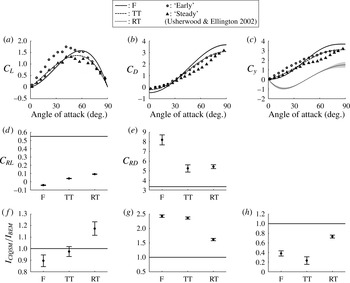
Figure 11. Coefficients for CIQSM calculated using 23 input cases. (a–c) The lift, drag and normal force coefficients for CIQSM. The experimental values of Usherwood & Ellington (Reference Usherwood and Ellington2002) are shown for comparisons. (d–e) Rotational lift and drag coefficients. The $C_{RL}$
by Zheng et al. (Reference Zheng, Hedrick and Mittal2013) and maximum drag coefficients by Usherwood & Ellington (Reference Usherwood and Ellington2002) are shown for comparison. (f–h) Ratio of the shape-dependent coefficients for added mass forces (f)
$C_{RL}$
by Zheng et al. (Reference Zheng, Hedrick and Mittal2013) and maximum drag coefficients by Usherwood & Ellington (Reference Usherwood and Ellington2002) are shown for comparison. (f–h) Ratio of the shape-dependent coefficients for added mass forces (f) $I_{am1}$
, (g)
$I_{am1}$
, (g) $I_{am2}$
and (h)
$I_{am2}$
and (h) $I_{am3}$
by CIQSM and BEM. The shaded region around lines and error bars display the standard deviation.
$I_{am3}$
by CIQSM and BEM. The shaded region around lines and error bars display the standard deviation.
The coefficients of the normal force $C_{y}$
by translational circulation and drag, which is used for calculating the rotational torque, are shown in figure 11(c). The
$C_{y}$
by translational circulation and drag, which is used for calculating the rotational torque, are shown in figure 11(c). The $C_{y}$
for force and translational torque are also shown for comparison. As the chordwise location of the centre of the pressure shifts from leading to trailing edge with increasing angle of attack (Dickson et al.
Reference Dickson, Straw and Dickinson2008), the
$C_{y}$
for force and translational torque are also shown for comparison. As the chordwise location of the centre of the pressure shifts from leading to trailing edge with increasing angle of attack (Dickson et al.
Reference Dickson, Straw and Dickinson2008), the $C_{y}$
for rotational torque is significantly lower than the
$C_{y}$
for rotational torque is significantly lower than the $C_{y}$
for force and translational torque. The
$C_{y}$
for force and translational torque. The $C_{y}$
can be negative when the angle of attack is lower than approximately 40°, because, with this wing shape, the centre of pressure moves towards the leading edge beyond the wing pivot axis. The standard deviation in
$C_{y}$
can be negative when the angle of attack is lower than approximately 40°, because, with this wing shape, the centre of pressure moves towards the leading edge beyond the wing pivot axis. The standard deviation in $C_{y}$
is slightly higher than that in
$C_{y}$
is slightly higher than that in $C_{L}$
,
$C_{L}$
, $C_{D}$
or
$C_{D}$
or $C_{y}$
for force and translational torque, which may suggest that the chordwise location of the LEV, and hence the rotational torque, is quite sensitive to the wing kinematics, and the effect of factors other than the angle of attack which may be missing from the model.
$C_{y}$
for force and translational torque, which may suggest that the chordwise location of the LEV, and hence the rotational torque, is quite sensitive to the wing kinematics, and the effect of factors other than the angle of attack which may be missing from the model.
The coefficients of rotational circulation $C_{RL}$
and drag
$C_{RL}$
and drag $C_{RD}$
for force, translational torque and rotational torque are presented in figure 11(d,e). The
$C_{RD}$
for force, translational torque and rotational torque are presented in figure 11(d,e). The $C_{RL}$
becomes significantly lower than experimental or fitted values (Sane & Dickinson Reference Sane and Dickinson2002; Zheng et al.
Reference Zheng, Hedrick and Mittal2013), while the rotational drag is higher than the maximum value of the coefficient for translational drag of Usherwood & Ellington (Reference Usherwood and Ellington2002). These differences are likely to be because rotational drag is newly taken into account in this study and the force associated with the rotational velocity is dominated by the drag in our morphological and kinematic models.
$C_{RL}$
becomes significantly lower than experimental or fitted values (Sane & Dickinson Reference Sane and Dickinson2002; Zheng et al.
Reference Zheng, Hedrick and Mittal2013), while the rotational drag is higher than the maximum value of the coefficient for translational drag of Usherwood & Ellington (Reference Usherwood and Ellington2002). These differences are likely to be because rotational drag is newly taken into account in this study and the force associated with the rotational velocity is dominated by the drag in our morphological and kinematic models.
Figure 11(f–h) illustrates the ratio of shape-dependent coefficients for the force due to added mass for the CIQSM and the BEM. While $I_{am1}$
for CIQSM is close to that for BEM,
$I_{am1}$
for CIQSM is close to that for BEM, $I_{am2}$
and
$I_{am2}$
and $I_{am3}$
, which are associated with the velocity and rotational acceleration, are much lower or higher than those from the BEM. Because the force due to added mass in the BEM is based on a two-dimensional wing in inviscid fluid (Sane & Dickinson Reference Sane and Dickinson2002), our coefficients are tuned for a more realistic, three-dimensional case.
$I_{am3}$
, which are associated with the velocity and rotational acceleration, are much lower or higher than those from the BEM. Because the force due to added mass in the BEM is based on a two-dimensional wing in inviscid fluid (Sane & Dickinson Reference Sane and Dickinson2002), our coefficients are tuned for a more realistic, three-dimensional case.
4. Demonstration of the CIQSM: aerodynamic power minimization
The results in the previous section showed that the CIQSM is an effective tool for tuning the wing kinematics in terms of its accuracy. In order to clearly demonstrate the concept and to give an impression of the parameter ranges that this particular model can cover, an optimization of wing kinematics for a morphological model of a hawkmoth is performed. The wing kinematics for the optimization are expressed by positional and feathering angles on a horizontal stroke plane with the form of Fourier series as follows:
 $$\begin{eqnarray}\displaystyle & \displaystyle {\it\phi}=a_{p}\cos \left(2{\rm\pi}ft\right)\!, & \displaystyle\end{eqnarray}$$
 $$\begin{eqnarray}\displaystyle & \displaystyle {\it\alpha}=a_{f0}+\mathop{\sum }_{i}^{3}\left(a_{fi}\cos \left(2{\rm\pi}\text{i}ft\right)+b_{fi}\sin \left(2{\rm\pi}\text{i}ft\right)\right)\!. & \displaystyle\end{eqnarray}$$ $a_{p}$
,
$a_{p}$
, $a_{f0-3}$
,
$a_{f0-3}$
, $b_{f1-3}$
and frequency,
$b_{f1-3}$
and frequency, $f$
) are tuned by using the hybrid of a genetic algorithm and the simplex algorithm, following the method by Berman & Wang (Reference Berman and Wang2007). In this study, the algorithm is designed to run under three constraints: (1) weight support (cycle-averaged vertical force divided by mass) must be higher than 1, while the mass is assumed to be 1579 mg (Willmott & Ellington Reference Willmott and Ellington1997), (2) cycle-averaged horizontal force must be lower than 10 % of weight, and (3) the wing beat amplitude must be less than 120° (based on hawkmoth wing kinematics). The first and second constraints are required for hovering, while the last constraint is added because wing beat amplitude tends to reach the maximum allowed values for power minimization (Berman & Wang Reference Berman and Wang2007). The initial parameters for the procedure are chosen randomly from the possible range of each parameter (
$f$
) are tuned by using the hybrid of a genetic algorithm and the simplex algorithm, following the method by Berman & Wang (Reference Berman and Wang2007). In this study, the algorithm is designed to run under three constraints: (1) weight support (cycle-averaged vertical force divided by mass) must be higher than 1, while the mass is assumed to be 1579 mg (Willmott & Ellington Reference Willmott and Ellington1997), (2) cycle-averaged horizontal force must be lower than 10 % of weight, and (3) the wing beat amplitude must be less than 120° (based on hawkmoth wing kinematics). The first and second constraints are required for hovering, while the last constraint is added because wing beat amplitude tends to reach the maximum allowed values for power minimization (Berman & Wang Reference Berman and Wang2007). The initial parameters for the procedure are chosen randomly from the possible range of each parameter ( $a_{p}$
: 0 to 60°,
$a_{p}$
: 0 to 60°, $a_{f0}$
:
$a_{f0}$
: $-45$
to 45°,
$-45$
to 45°, $a_{f1-3}$
,
$a_{f1-3}$
, $b_{f1-3}$
:
$b_{f1-3}$
: $-90$
to 90°,
$-90$
to 90°, $f$
: 1–100 Hz). Note that the range of
$f$
: 1–100 Hz). Note that the range of $a_{f0}$
is set to be smaller than the other parameters in order to avoid kinematics with alternating leading edges (Berman & Wang Reference Berman and Wang2007). The CIQSM is constructed with all of the kinematics shown in figure 4.
$a_{f0}$
is set to be smaller than the other parameters in order to avoid kinematics with alternating leading edges (Berman & Wang Reference Berman and Wang2007). The CIQSM is constructed with all of the kinematics shown in figure 4.
The results of the power minimization are summarized in figure 12 and table 2. Wing beat amplitude is equal to 120° ( $=$
2.0944 rad) as expected. The wing motion is nearly symmetric because the offset (
$=$
2.0944 rad) as expected. The wing motion is nearly symmetric because the offset ( $a_{f0}$
) and second terms (
$a_{f0}$
) and second terms ( $a_{f2}$
and
$a_{f2}$
and $b_{f2}$
) of the Fourier series of feathering angle are close to zero. Unlike hawkmoth kinematics that generates two peaks in force and power during each half-stroke, one distinct peak at late downstroke is generated by the optimized kinematics. We have also evaluated the optimized kinematics with CFD in order to test the accuracy of the prediction by CIQSM. As shown in figure 12(c,d), the dynamic force and power by CIQSM closely match with the CFD. The discrepancy between the models is higher early in the half-stroke, most likely because of wing–wake interactions. Also, the CIQSM slightly underestimates the peak force and power. As a result, the errors in the mean vertical force and power are
$b_{f2}$
) of the Fourier series of feathering angle are close to zero. Unlike hawkmoth kinematics that generates two peaks in force and power during each half-stroke, one distinct peak at late downstroke is generated by the optimized kinematics. We have also evaluated the optimized kinematics with CFD in order to test the accuracy of the prediction by CIQSM. As shown in figure 12(c,d), the dynamic force and power by CIQSM closely match with the CFD. The discrepancy between the models is higher early in the half-stroke, most likely because of wing–wake interactions. Also, the CIQSM slightly underestimates the peak force and power. As a result, the errors in the mean vertical force and power are $-6.8$
% and
$-6.8$
% and $-12.6$
% of CFD predictions. These errors are slightly higher than the estimate in the previous section, probably because the optimized kinematics sit outside the input parameter space for the CIQSM and are therefore an extrapolation. However, it should be emphasized that the accuracy of the optimization is significantly improved compared with the BEM-based optimization.
$-12.6$
% of CFD predictions. These errors are slightly higher than the estimate in the previous section, probably because the optimized kinematics sit outside the input parameter space for the CIQSM and are therefore an extrapolation. However, it should be emphasized that the accuracy of the optimization is significantly improved compared with the BEM-based optimization.
Zheng et al. (Reference Zheng, Hedrick and Mittal2013) optimized the wing kinematics by using a BEM in order to maximize the power loading. Interestingly, even though various conditions are different, the optimization resulted in a horizontal wing stroke, which is similar to the current study. The optimized force and power by the BEM matched the CFD result qualitatively, but the BEM substantially overestimated both vertical force and power consumption. The tuning of the quasi-steady model based on high-fidelity modelling accounts for the improvement in the accuracy, and therefore can greatly expand the applicability of quasi-steady models.

Figure 12. Optimized wing kinematics and its aerodynamic performances. (a) Angular motion of the cross-section during downstroke and upstroke. Circles show the leading edges of the cross-sections. (b) Time courses of the optimized flapping angles. (c,d) Time courses of the aerodynamic vertical force and aerodynamic power with optimized wing kinematics calculated by the CIQSM and CFD. The mean values are shown by the horizontal lines in each panel.
Table 2. Optimized kinematic parameters. Angles are given in radians.

5. Further remarks and conclusion
The demonstration with power minimization and the probability distributions of the errors and PCCs in figure 9 indicate that the CIQSM outperforms the conventional BEM in terms of its accuracy. In fact, previous studies could not achieve such low errors and high PCCs between BEM and CFD. For example, Berman & Wang (Reference Berman and Wang2007) compared the prediction by BEM and CFD models of fruitflies, bumblebees and hawkmoths by Sun & Du (Reference Sun and Du2003), and their quasi-steady model agrees with their CFD predictions to within approximately 15 %, which is higher than the error we present here. Zheng et al. (Reference Zheng, Hedrick and Mittal2013) performed 22 BEM and CFD analyses with different wing kinematics, and the PCCs of mean vertical force and power were 0.79 and 0.91, respectively. However, it should be noted that it is difficult to rigorously compare the accuracy of the current model with previous quasi-steady models due to the absence of a standard test case.
The improvement in performance is achieved by taking into account the effect of wake interaction and three-dimensional effects by fitting coefficients from a high-fidelity model. The flapping wing in hover travels through the distributed downwash created by the previous strokes, and hence the angle of attack can be reduced. The wing tip vortex can reduce the pressure difference between upper and lower surfaces around the wing tip. Lift and drag coefficients that have been measured on physical models of continuously spinning wings (e.g. Dickinson et al. Reference Dickinson, Lehmann and Sane1999; Usherwood & Ellington Reference Usherwood and Ellington2002) include these effects reasonably well, while the coefficients in our CIQSM are the results of a more realistic, reciprocating motion. Moreover, it is not accurate to use coefficients from a BEM for estimating torques and power because of error in the position of the centre of pressure. The aerodynamic power is separately modelled in this study, rather than being based on the assumption that the aerodynamic force coefficients are the same at all points on the wing, so, uniquely, the power predictions from our CIQSM are independent of the force coefficients. Therefore, both the force and power predictions from our model inherently include the effects of downwash and the wing tip vortex.
The accuracy of the CIQSM is wholely dependent on the accuracy of the CFD model that is used for tuning the quasi-steady model. Therefore, it is possible that the coefficients shown in figure 11 are modified if another simulator is used to construct the CIQSM. However, because the current simulator is well validated (Liu Reference Liu2009; Nakata & Liu Reference Nakata and Liu2012) through comparison with experimental results (Dickinson et al. Reference Dickinson, Lehmann and Sane1999; Heathcote & Gursul Reference Heathcote and Gursul2007; Heathcote, Wang & Gursul Reference Heathcote, Wang and Gursul2008; Lua et al. Reference Lua, Lai, Lim and Yep2010) and those have been compared with CFD simulations from other groups extensively (e.g. Ramamuti & Sandberg Reference Ramamuti and Sandberg2002; Sun & Tang Reference Sun and Tang2002; Chimakurthi et al. Reference Chimakurthi, Tang, Palacios, Cesnik and Shyy2009; Dai, Luo & Doyle Reference Dai, Luo and Doyle2012; Grodnier et al. Reference Grodnier, Chimakurthi, Cesnik and Attar2013; Le et al. Reference Le, Truong, Park, Truong, Ko, Park and Byun2013; Wan, Dong & Gai Reference Wan, Dong and Gai2015), we can be confident that the CIQSM will be effective even if the model is constructed using data from other high-fidelity models.
The discussion in § 3.2 with figure 8 shows that, while utilizing the simplicity of the quasi-steady model, the current CIQSM cannot predict large changes in aerodynamic performance due to the transitions between regimes in the flow structure because it is based on the quasi-steady assumption. For example, the effect of Reynolds number on lift and drag coefficients (Lentink & Dickinson Reference Lentink and Dickinson2009) needs to be modelled in order to apply the CIQSM across a wide range of Reynolds numbers. More generally, since the CIQSM is an interpolation of high-fidelity results similar to surrogate modelling (Queipo et al. Reference Queipo, Haftka, Shyy, Goel, Vaidyanathan and Tucker2005), the model will be less accurate in predicting aerodynamic performance if the wing shape, kinematics, Reynolds number or flight mode is extrapolated very far from the input models. This does not limit its utility but serves as a useful guideline when choosing the number and extent of input cases. In its present form, one of the possible ways to use the CIQSM is for finely tuning wing kinematics to minimize power consumption or for trimming hovering flight after performing several high-fidelity simulations. Such issues present a significant challenge for high-fidelity models, even if searching a parameter space close to the input baseline cases, because of the complexity of flapping-wing motions. However, this becomes feasible using the CIQSM.
In summary, we present a new model of flapping-wing aerodynamics, called a CIQSM, based on combining CFD data with quasi-steady modelling. By comparing the model’s predictions with those of high-fidelity CFD and a BEM, it was found that the mean vertical force and aerodynamic power predicted by the CIQSM match the CFD results more accurately than the BEM over a range of Reynolds numbers from 80 % to 120 %, varied by wing beat amplitude or frequency. The conclusion is based on the model of a hovering hawkmoth that is a well known example of a flapping-wing flyer. Good matches between the predictions by quasi-steady and high-fidelity models shown by previous reports (Berman & Wang Reference Berman and Wang2007; Nabawy & Crowther Reference Nabawy and Crowther2014b ) promise the widespread applicability of the current methodology. The CIQSM is particularly useful for studies that require the exploration of a parameter space – for example, the optimization of wing kinematics, wing shape or flight control strategies – because it is computationally cheap once it has been parameterized by a relatively small set of high-fidelity analyses.
Acknowledgements
This work was supported by EPSRC grant (EP/H004025/1), BBSRC grant (BB/J001244/1) and an EPSRC Career Acceleration Fellowship to R.J.B., and by a Grant-in-Aid for Scientific Research on Innovative Areas (24120007, JSPS) to H.L. The authors would like to acknowledge the use of the University of Oxford Advanced Research Computing (ARC) facility in carrying out this work (http://dx.doi.org/10.5281/zenodo.22558).


 Open access