


1. Introduction
It is well known that small heavy particles with large Stokes number dampen turbulence (Tsuji, Morikawa & Shiomi Reference Tsuji, Morikawa and Shiomi1984; Gore & Crowe Reference Gore and Crowe1989; Hetseroni Reference Hetseroni1989; Elghobashi & Truesdell Reference Elghobashi and Truesdell1993; Kulick, Fessler & Eaton Reference Kulick, Fessler and Eaton1994; Li et al.
Reference Li, McLaughlin, Kontomaris and Portela2001; Yamamoto et al.
Reference Yamamoto, Potthoff, Tanaka, Kajishima and Tsuji2001; Ferrante & Elghobashi Reference Ferrante and Elghobashi2003; Mito & Hanratty Reference Mito and Hanratty2006; Vreman Reference Vreman2007). In their experiments on particle-laden plane channel flow, Kulick et al. (Reference Kulick, Fessler and Eaton1994) reported a strong attenuation of the air turbulence intensity at low solid volume fraction but significant solid mass loading. Particularly strong turbulence attenuation, 75 % reduction of the streamwise gas velocity fluctuation at the centreline, was observed for copper particles of
 $70~{\rm\mu}\text{m}$
at a mass loading ratio of 0.8. The Reynolds number of the unladen case based on friction velocity and channel half-width was
$70~{\rm\mu}\text{m}$
at a mass loading ratio of 0.8. The Reynolds number of the unladen case based on friction velocity and channel half-width was
 $Re_{{\it\tau}}=644$
. Compared with the scale of the turbulence, the copper particle diameter was small (
$Re_{{\it\tau}}=644$
. Compared with the scale of the turbulence, the copper particle diameter was small (
 $d_{p}^{+}\approx 2.3$
, where
$d_{p}^{+}\approx 2.3$
, where
 $d_{p}^{+}$
denotes the particle diameter
$d_{p}^{+}$
denotes the particle diameter
 $d_{p}$
in wall units). An understanding of the mechanisms of the turbulence modification by particles is far from trivial, because there are so many different interactions and mechanisms involved: physical instabilities, turbulence, particle–fluid interactions, particle–particle interactions and particle–wall interactions. Particle–wall interactions are influenced by complicated factors like electrostatic effects and wall roughness.
$d_{p}$
in wall units). An understanding of the mechanisms of the turbulence modification by particles is far from trivial, because there are so many different interactions and mechanisms involved: physical instabilities, turbulence, particle–fluid interactions, particle–particle interactions and particle–wall interactions. Particle–wall interactions are influenced by complicated factors like electrostatic effects and wall roughness.
The experimental work of Kulick et al. (Reference Kulick, Fessler and Eaton1994), hereafter referred to as KFE1994, has frequently been used for comparison with results of numerical simulations of vertical (downward) particle-laden channel flows (Wang & Squires Reference Wang and Squires1996; Li et al. Reference Li, McLaughlin, Kontomaris and Portela2001; Rouson & Eaton Reference Rouson and Eaton2001; Yamamoto et al. Reference Yamamoto, Potthoff, Tanaka, Kajishima and Tsuji2001; Segura Reference Segura2004; Kubik & Kleiser Reference Kubik and Kleiser2006). In all these simulations the Eulerian–Lagrangian method was used. Simulations of this type solve the (incompressible) Navier–Stokes equations in the Eulerian frame for the continuous phase and solve Lagrangian equations for the dispersed phase. The particles are treated as point particles, and a correlation for the force of the fluid on the particle is applied. This means that the boundary layers on the particle surfaces are not resolved. Dependent on whether the equations of the continuous phase are solved with large-eddy simulation (LES) or with direct numerical simulation (DNS), we call the Euler–Lagrangian method point-particle LES (PP-LES) or point-particle DNS (PP-DNS). Thus, in PP-LES only the large-scale turbulence is resolved, while in PP-DNS, apart from particle boundary layers and wakes, all scales of the flow are resolved. This name has been chosen to contrast the method with particle-resolved DNS, in which also the boundary layers on the particle surfaces are fully resolved.
An important difference between the experiments of KFE1994 and simulations of these experiments reported in the literature is that the mean particle velocity in the experiments was much lower than in the simulations. Experiments of Benson, Tanaka & Eaton (Reference Benson, Tanaka and Eaton2005) showed that the relatively low mean particle velocities in the experiments of KFE1994 were most probably due to rough walls in the development section of the flow, approximately 30 cm upstream of the measurement location. In addition, Benson et al. (Reference Benson, Tanaka and Eaton2005) performed measurements for fully rough walls, i.e. a case in which the measurement location had been moved very close to the rough development section. In the fully rough case, the streamwise turbulence intensity of the gas phase was not attenuated but amplified. The mass loading ratio was 0.15, and the roughness height was
 $250~{\rm\mu}\text{m}$
, approximately eight times the viscous length scale. The effects of much smaller roughness heights were investigated by Kussin & Sommerfeld (Reference Kussin and Sommerfeld2002); however, not for vertical but for horizontal particle-laden channel flow. In these experiments, the turbulence was not amplified by the rough walls; in contrast, turbulence attenuation became stronger with increasing wall roughness. The smallest particle diameter for which this effect was observed was
$250~{\rm\mu}\text{m}$
, approximately eight times the viscous length scale. The effects of much smaller roughness heights were investigated by Kussin & Sommerfeld (Reference Kussin and Sommerfeld2002); however, not for vertical but for horizontal particle-laden channel flow. In these experiments, the turbulence was not amplified by the rough walls; in contrast, turbulence attenuation became stronger with increasing wall roughness. The smallest particle diameter for which this effect was observed was
 $100~{\rm\mu}\text{m}$
(
$100~{\rm\mu}\text{m}$
(
 $d_{p}^{+}\approx 5.4$
) and the corresponding turbulence attenuation of the streamwise gas velocity fluctuation at the centreline was approximately 30 % for the highest wall roughness at a mass loading ratio of 0.7. In view of this literature, our first research question is then whether turbulence attenuation in vertical particle-laden channel flow can be enhanced by rough walls.
$d_{p}^{+}\approx 5.4$
) and the corresponding turbulence attenuation of the streamwise gas velocity fluctuation at the centreline was approximately 30 % for the highest wall roughness at a mass loading ratio of 0.7. In view of this literature, our first research question is then whether turbulence attenuation in vertical particle-laden channel flow can be enhanced by rough walls.
The effect of wall roughness on particle-laden turbulence has also been addressed in various simulation studies, see for example Sommerfeld (Reference Sommerfeld1992), Squires & Simonin (Reference Squires and Simonin2006), Vreman (Reference Vreman2007), Konan, Simonin & Squires (Reference Konan, Simonin and Squires2011), Breuer, Alletto & Langfeldt (Reference Breuer, Alletto and Langfeldt2012) and Alletto & Breuer (Reference Alletto and Breuer2013). In these works stochastic models for the particle–wall collisions were used. The stochastic wall roughness model of Breuer et al. (Reference Breuer, Alletto and Langfeldt2012) is based on model-inherent geometric relations which are theoretically implied if the wall roughness has the geometry of a layer of fixed spheres. An important geometric relation that is taken into account is the so-called shadow effect (Sommerfeld & Huber Reference Sommerfeld and Huber1999), which means that particles that approach the wall with a given angle cannot reach particular regions of the rough wall (shadowed regions). However, no simulation study, in particular no PP-DNS study, could be found in which the effects of smooth and rough walls on the particle-induced turbulence attenuation were compared.
Turbulence attenuation has also been simulated for downward particle-laden pipe flow, with use of PP-DNS up to a mass loading ratio of 1.1 (Vreman Reference Vreman2007). These simulations were inspired by the experiments of Caraman, Borée & Simonin (Reference Caraman, Borée and Simonin2003) and Borée & Caraman (Reference Borée and Caraman2005). The Reynolds number based on friction velocity and pipe radius was
 $Re_{{\it\tau}}=140$
, lower than the Reynolds number in KFE1994. In addition to PP-DNS, a simplified simulation was performed by Vreman (Reference Vreman2007): DNS of a pipe flow forced by a linear term, proportional to the relative velocity between the phases. No explicit particles were included; instead, the particle velocity was prescribed, such that the streamwise component was constant in space and time and the other components were zero. Strong turbulence attenuation was observed, even if the linear forcing term was just proportional to the mean relative velocity between the phases. The key feature of the simple forcing term was its non-uniformity in the wall-normal direction; the force was positive near the wall and negative at the centre.
$Re_{{\it\tau}}=140$
, lower than the Reynolds number in KFE1994. In addition to PP-DNS, a simplified simulation was performed by Vreman (Reference Vreman2007): DNS of a pipe flow forced by a linear term, proportional to the relative velocity between the phases. No explicit particles were included; instead, the particle velocity was prescribed, such that the streamwise component was constant in space and time and the other components were zero. Strong turbulence attenuation was observed, even if the linear forcing term was just proportional to the mean relative velocity between the phases. The key feature of the simple forcing term was its non-uniformity in the wall-normal direction; the force was positive near the wall and negative at the centre.
Indeed, in wall-bounded gas–solid flow, the mean profile of the relative velocity of the phases is usually not constant in the wall-normal direction. Since the density of the particles is much larger than the density of the gas, a particle that moves from the bulk region to the wall will in general not have lost all its streamwise momentum when it arrives at the wall. As a result, the mean particle velocity profile is usually flatter than the mean fluid velocity profile, such that the mean relative velocity is non-uniform in the wall-normal direction. Consequently, the feedback force, the mean force exerted by the particles on the gas, is also non-uniform in the wall-normal direction (at least if the particle concentration is uniform). The non-uniformity is relatively strong in channels with rough walls; experiments indicate that the particle velocity profile is flatter for rough than for smooth walls (Benson et al. Reference Benson, Tanaka and Eaton2005). Is a change of turbulence attenuation with increased wall roughness perhaps related to increased non-uniformity of the mean feedback force? It is not evident that the non-uniformity of the mean feedback force is relevant for turbulence attenuation, since the turbulence kinetic energy equation for particle-laden flow does not contain a term with the mean feedback force. This leads to the second research question of the present paper: what role does the non-uniform part of the mean feedback force play in particle-laden channel flows at conditions comparable to the KFE1994 experiments? Is the finding that the non-uniform mean feedback force is one of the mechanisms that leads to turbulence attenuation in particle-laden pipe flow at low Reynolds number (Vreman Reference Vreman2007) also valid for particle-laden channel flow at at least four times larger Reynolds number?
To answer the two research questions formulated above, we perform PP-DNS of downward particle-laden flow in smooth and rough vertical channels. For reasons mentioned in the next section, inter-particle collisions are included in the simulations. The Reynolds number
 $Re_{{\it\tau}}$
is 642 and the mass loading ratio is 0.8, such that the simulations correspond to the case with the strongest turbulence attenuation in KFE1994. To investigate the effect of the mean feedback force on turbulence attenuation, PP-DNS results will be compared with DNS results of single-phase channel flow with non-uniform streamwise forcing. The non-uniform forcing in each of the latter simulations is a function of the wall-normal coordinate only and is prescribed by the mean feedback force extracted from a PP-DNS. The experiments of Kussin & Sommerfeld (Reference Kussin and Sommerfeld2002) have not been selected as reference cases for the simulations, because of the first research question, but also because the turbulence attenuation observed in these experiments was less strong than in KFE1994. In addition, PP-DNS of the most relevant case for turbulence attenuation from Kussin & Sommerfeld (Reference Kussin and Sommerfeld2002) has to deal with the complications of even higher Reynolds number (
$Re_{{\it\tau}}$
is 642 and the mass loading ratio is 0.8, such that the simulations correspond to the case with the strongest turbulence attenuation in KFE1994. To investigate the effect of the mean feedback force on turbulence attenuation, PP-DNS results will be compared with DNS results of single-phase channel flow with non-uniform streamwise forcing. The non-uniform forcing in each of the latter simulations is a function of the wall-normal coordinate only and is prescribed by the mean feedback force extracted from a PP-DNS. The experiments of Kussin & Sommerfeld (Reference Kussin and Sommerfeld2002) have not been selected as reference cases for the simulations, because of the first research question, but also because the turbulence attenuation observed in these experiments was less strong than in KFE1994. In addition, PP-DNS of the most relevant case for turbulence attenuation from Kussin & Sommerfeld (Reference Kussin and Sommerfeld2002) has to deal with the complications of even higher Reynolds number (
 $Re_{{\it\tau}}=950$
) and larger
$Re_{{\it\tau}}=950$
) and larger
 $d_{p}^{+}$
(the errors in the particle drag force correlation increase with
$d_{p}^{+}$
(the errors in the particle drag force correlation increase with
 $d_{p}^{+}$
).
$d_{p}^{+}$
).
Unlike in the references mentioned above, no stochastic wall roughness model is used in the simulations. Instead, the walls in the rough cases are covered with tiny fixed spherical ‘wall particles’ of diameter
 $d_{p,w}$
, and all collisions between free particles and wall particles are taken into account. A similar type of roughness has been used in experiments (Ligrani & Moffat Reference Ligrani and Moffat1986). In single-phase flow, the effect of wall roughness on turbulence can usually be ignored if the roughness size is less than five wall units (Jimenez Reference Jimenez2004). Indeed, experiments on single-phase boundary layers have shown that the effects of roughness on single-phase turbulence are negligible, if
$d_{p,w}$
, and all collisions between free particles and wall particles are taken into account. A similar type of roughness has been used in experiments (Ligrani & Moffat Reference Ligrani and Moffat1986). In single-phase flow, the effect of wall roughness on turbulence can usually be ignored if the roughness size is less than five wall units (Jimenez Reference Jimenez2004). Indeed, experiments on single-phase boundary layers have shown that the effects of roughness on single-phase turbulence are negligible, if
 $k_{rms}^{+}<0.5$
and
$k_{rms}^{+}<0.5$
and
 $k_{l}^{+}<10$
(Flack & Schultz Reference Flack and Schultz2014), where
$k_{l}^{+}<10$
(Flack & Schultz Reference Flack and Schultz2014), where
 $k_{rms}$
is the root-mean-square fluctuation of the surface elevation and
$k_{rms}$
is the root-mean-square fluctuation of the surface elevation and
 $k_{l}$
is the peak-to-trough roughness height. In this regime, surface elements do not modify the skin friction in single-phase flow, since viscosity damps out eddies created by the surface roughness elements (Flack & Schultz Reference Flack and Schultz2014). The wall roughness in the present simulations satisfies
$k_{l}$
is the peak-to-trough roughness height. In this regime, surface elements do not modify the skin friction in single-phase flow, since viscosity damps out eddies created by the surface roughness elements (Flack & Schultz Reference Flack and Schultz2014). The wall roughness in the present simulations satisfies
 $k_{rms}^{+}\leqslant 0.11$
and
$k_{rms}^{+}\leqslant 0.11$
and
 $k_{l}^{+}\leqslant 0.32$
and is therefore sufficiently small to allow smooth boundary conditions for the gas phase. Thus, in the simulations the wall roughness can modify the gas turbulence only via the particles.
$k_{l}^{+}\leqslant 0.32$
and is therefore sufficiently small to allow smooth boundary conditions for the gas phase. Thus, in the simulations the wall roughness can modify the gas turbulence only via the particles.
The structure of the paper is as follows. In § 2, we introduce the flow cases, describe the PP-DNS method and discuss the modelling assumptions. In § 3, we present the results of the PP-DNS, for smooth and rough channels, to show the effect of wall roughness on turbulence attenuation. Results are shown for the decomposition of the feedback force in a mean uniform, a mean non-uniform and a fluctuating part. The streamwise mean momentum equation is analysed. In addition, the turbulence kinetic energy budgets are compared. In § 4, we present results of non-uniformly forced DNS of single-phase channel flow to demonstrate the isolated effect of a non-uniform mean feedback force. In addition, we perform a linear stability analysis of the effect of a linear feedback force on the instability of laminar particle-laden channel flow, also for a case in which the mean feedback force is non-uniform. Finally, the conclusions are summarized in § 5.
2. Flow cases and method
2.1. Simulation cases
To investigate the topics mentioned in the introduction, numerical simulations are performed. The configuration and parameters of the simulation cases are based on two experimental cases in KFE1994: the unladen case and the particle-laden case for which the strongest reduction of turbulence was measured. Although the basic presentation will be in dimensional variables, to retain the advantage of dimensional checking, the relevant non-dimensional numbers will be specified. Table 1 shows an overview of four simulations, A0–A3. The unladen flow (A0) is a turbulent channel flow at Reynolds number
 $Re_{{\it\tau}}=642$
, based on channel half-width
$Re_{{\it\tau}}=642$
, based on channel half-width
 $H=0.02~\text{m}$
, wall friction velocity
$H=0.02~\text{m}$
, wall friction velocity
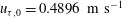 $u_{{\it\tau},0}=0.4896~\text{m}~\text{s}^{-1}$
and kinematic viscosity
$u_{{\it\tau},0}=0.4896~\text{m}~\text{s}^{-1}$
and kinematic viscosity
 ${\it\nu}=1.525\times 10^{-5}~\text{m}^{2}~\text{s}^{-1}$
. Thus, the viscous length scale of the reference flow is equal to
${\it\nu}=1.525\times 10^{-5}~\text{m}^{2}~\text{s}^{-1}$
. Thus, the viscous length scale of the reference flow is equal to
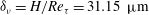 ${\it\delta}_{{\it\nu}}=H/Re_{{\it\tau}}=31.15~{\rm\mu}\text{m}$
. The centreline velocity equals
${\it\delta}_{{\it\nu}}=H/Re_{{\it\tau}}=31.15~{\rm\mu}\text{m}$
. The centreline velocity equals
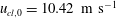 $u_{cl,0}=10.42~\text{m}~\text{s}^{-1}$
and the bulk velocity is
$u_{cl,0}=10.42~\text{m}~\text{s}^{-1}$
and the bulk velocity is
 $9.212~\text{m}~\text{s}^{-1}$
. In addition, the gas is air with a constant density of
$9.212~\text{m}~\text{s}^{-1}$
. In addition, the gas is air with a constant density of
 ${\it\rho}=1.2~\text{kg}~\text{m}^{-3}$
, and the flow in the vertically positioned channel is downward (gravity acceleration
${\it\rho}=1.2~\text{kg}~\text{m}^{-3}$
, and the flow in the vertically positioned channel is downward (gravity acceleration
 $g=9.8~\text{m}~\text{s}^{-2}$
). The diameter of the (free) particles in the laden cases is
$g=9.8~\text{m}~\text{s}^{-2}$
). The diameter of the (free) particles in the laden cases is
 $d_{p}=70~{\rm\mu}\text{m}$
, and the density of the particles is the density of copper,
$d_{p}=70~{\rm\mu}\text{m}$
, and the density of the particles is the density of copper,
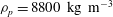 ${\it\rho}_{p}=8800~\text{kg}~\text{m}^{-3}$
. The Stokes response time,
${\it\rho}_{p}=8800~\text{kg}~\text{m}^{-3}$
. The Stokes response time,
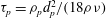 ${\it\tau}_{p}={\it\rho}_{p}d_{p}^{2}/(18{\it\rho}{\it\nu})$
, is equal to 0.131 s, which corresponds to a Stokes number
${\it\tau}_{p}={\it\rho}_{p}d_{p}^{2}/(18{\it\rho}{\it\nu})$
, is equal to 0.131 s, which corresponds to a Stokes number
 ${\it\tau}_{p}u_{{\it\tau},0}/{\it\delta}_{{\it\nu}}\approx 2060$
. The particle diameter is small compared with the length scale of most turbulent eddies,
${\it\tau}_{p}u_{{\it\tau},0}/{\it\delta}_{{\it\nu}}\approx 2060$
. The particle diameter is small compared with the length scale of most turbulent eddies,
 $d_{p}\approx 0.45{\it\eta}$
at the centre and
$d_{p}\approx 0.45{\it\eta}$
at the centre and
 $d_{p}\approx 1.55{\it\eta}$
at the wall, where
$d_{p}\approx 1.55{\it\eta}$
at the wall, where
 ${\it\eta}=({\it\nu}^{3}/{\it\epsilon})^{1/4}$
is the Kolmogorov length scale, based on the unladen turbulence dissipation rate (
${\it\eta}=({\it\nu}^{3}/{\it\epsilon})^{1/4}$
is the Kolmogorov length scale, based on the unladen turbulence dissipation rate (
 ${\it\epsilon}$
), which is a function of the distance to the nearest wall. The domain-averaged solid volume fraction of the particles is the same in the three laden cases, namely
${\it\epsilon}$
), which is a function of the distance to the nearest wall. The domain-averaged solid volume fraction of the particles is the same in the three laden cases, namely
 $1.092\times 10^{-4}$
. By definition, the mass loading ratio parameter
$1.092\times 10^{-4}$
. By definition, the mass loading ratio parameter
 ${\it\phi}$
is equal to the overall solid volume fraction multiplied by
${\it\phi}$
is equal to the overall solid volume fraction multiplied by
 ${\it\rho}_{p}/{\it\rho}$
, thus
${\it\rho}_{p}/{\it\rho}$
, thus
 ${\it\phi}=0.801$
(80 %). The walls are smooth in case A1 and rough in cases A2 and A3. The wall in case A3 is rougher than in case A2. The wall roughness will be defined in a separate section.
${\it\phi}=0.801$
(80 %). The walls are smooth in case A1 and rough in cases A2 and A3. The wall in case A3 is rougher than in case A2. The wall roughness will be defined in a separate section.
Table 1. The four simulation cases A0–A3.

2.2. The Eulerian–Lagrangian approach
The unladen case (A0) is simulated with DNS, while the laden cases (A1–A3) are simulated with an Eulerian–Lagrangian method, PP-DNS with two-way coupling and inter-particle collisions. For an introduction to the Eulerian–Lagrangian method, the reader is referred to Crowe, Sommerfeld & Tsuji (Reference Crowe, Sommerfeld and Tsuji1998), Deen et al. (Reference Deen, van Sint Annaland, van der Hoef and Kuipers2007) and van der Hoef et al. (Reference van der Hoef, van Sint Annaland, Deen and Kuipers2008). The method can be one-way coupled (the particle–fluid interaction appears in the particle equations only), two-way coupled (the particle–fluid interaction appears in the fluid and particle equations) or two-way coupled with inter-particle collisions included. In PP-LES studies of dilute vertical downward particle-laden channel flow at
 $Re_{{\it\tau}}\approx 640$
in the literature, all three types have been used: one-way coupling (Wang & Squires Reference Wang and Squires1996), two-way coupling (Segura Reference Segura2004) and two-way coupling with inter-particle collisions (Yamamoto et al.
Reference Yamamoto, Potthoff, Tanaka, Kajishima and Tsuji2001).
$Re_{{\it\tau}}\approx 640$
in the literature, all three types have been used: one-way coupling (Wang & Squires Reference Wang and Squires1996), two-way coupling (Segura Reference Segura2004) and two-way coupling with inter-particle collisions (Yamamoto et al.
Reference Yamamoto, Potthoff, Tanaka, Kajishima and Tsuji2001).
PP-DNS studies of vertical downward particle-laden plane channel flow in the literature were hitherto limited to lower Reynolds number:
 $Re_{{\it\tau}}=180$
with one-way coupling (Rouson & Eaton Reference Rouson and Eaton2001),
$Re_{{\it\tau}}=180$
with one-way coupling (Rouson & Eaton Reference Rouson and Eaton2001),
 $Re_{{\it\tau}}=210$
with two-way coupling (Kubik & Kleiser Reference Kubik and Kleiser2006), and
$Re_{{\it\tau}}=210$
with two-way coupling (Kubik & Kleiser Reference Kubik and Kleiser2006), and
 $Re_{{\it\tau}}=125$
(Li et al.
Reference Li, McLaughlin, Kontomaris and Portela2001) and
$Re_{{\it\tau}}=125$
(Li et al.
Reference Li, McLaughlin, Kontomaris and Portela2001) and
 $Re_{{\it\tau}}=150$
(Mito & Hanratty Reference Mito and Hanratty2006) with two-way coupling and inter-particle collisions. If we include PP-DNS of horizontal or non-gravitational particle-laden plane channel flows in our discussion, one-way coupled simulations of such flows were (for example) performed at
$Re_{{\it\tau}}=150$
(Mito & Hanratty Reference Mito and Hanratty2006) with two-way coupling and inter-particle collisions. If we include PP-DNS of horizontal or non-gravitational particle-laden plane channel flows in our discussion, one-way coupled simulations of such flows were (for example) performed at
 $Re_{{\it\tau}}=150$
(Pedinotti, Mariotti & Banerjee Reference Pedinotti, Mariotti and Banerjee1992; Marchioli & Soldati Reference Marchioli and Soldati2002),
$Re_{{\it\tau}}=150$
(Pedinotti, Mariotti & Banerjee Reference Pedinotti, Mariotti and Banerjee1992; Marchioli & Soldati Reference Marchioli and Soldati2002),
 $Re_{{\it\tau}}=300$
(Lavezzo et al.
Reference Lavezzo, Soldati, Gerashchenko, Warhaft and Collins2010) and
$Re_{{\it\tau}}=300$
(Lavezzo et al.
Reference Lavezzo, Soldati, Gerashchenko, Warhaft and Collins2010) and
 $Re_{{\it\tau}}=950$
(Geurts & Kuerten Reference Geurts and Kuerten2012; Kuerten & Brouwers Reference Kuerten and Brouwers2013), two-way coupled simulations up to
$Re_{{\it\tau}}=950$
(Geurts & Kuerten Reference Geurts and Kuerten2012; Kuerten & Brouwers Reference Kuerten and Brouwers2013), two-way coupled simulations up to
 $Re_{{\it\tau}}=395$
(Kuerten, van der Geld & Geurts Reference Kuerten, van der Geld and Geurts2011; Zhao, Andersson & Gillissen Reference Zhao, Andersson and Gillissen2013) and two-way coupled simulations with inter-particle collisions at
$Re_{{\it\tau}}=395$
(Kuerten, van der Geld & Geurts Reference Kuerten, van der Geld and Geurts2011; Zhao, Andersson & Gillissen Reference Zhao, Andersson and Gillissen2013) and two-way coupled simulations with inter-particle collisions at
 $Re_{{\it\tau}}=125$
(Nasr, Ahmadi & McLaughlin Reference Nasr, Ahmadi and McLaughlin2009).
$Re_{{\it\tau}}=125$
(Nasr, Ahmadi & McLaughlin Reference Nasr, Ahmadi and McLaughlin2009).
In view of the above review of the literature, PP-DNS with two-way coupling and inter-particle collisions is a state-of-the-art method to simulate particle-laden channel flow at
 $Re_{{\it\tau}}=642$
. For most particle-laden flows, including the present flow, it is not yet feasible to perform a DNS that resolves the boundary layers around the particles. In the class of feasible methods, two-way coupled PP-DNS with inter-particle collisions is probably the most advanced one. In addition, the present PP-DNS cases have several new features. First, although
$Re_{{\it\tau}}=642$
. For most particle-laden flows, including the present flow, it is not yet feasible to perform a DNS that resolves the boundary layers around the particles. In the class of feasible methods, two-way coupled PP-DNS with inter-particle collisions is probably the most advanced one. In addition, the present PP-DNS cases have several new features. First, although
 $Re_{{\it\tau}}=642$
is not high, the Reynolds number is approximately four times higher than in previous studies of turbulent channel flows using the same method (PP-DNS with two-way coupling and inter-particle collisions). Although a detailed study of the effect of Reynolds number falls outside the scope of this paper, the effect will be briefly addressed at the end of § 3.3. Second, it is the first time that wall roughness effects have been included in PP-DNS plane channel flow. It is not expected that the results would be very different if PP-LES at the same Reynolds number were used. Point-particle DNS has been chosen because it is feasible for this Reynolds number and it does reduce uncertainties caused by the simulation method to some extent, simply because the range of scales taken into account is larger than in PP-LES. Without correction, the turbulence intensity and turbulence kinetic energy in LES are generally lower than in DNS (how much lower depends on the resolution of the LES). Third, it is the first time that all interactions between the particles and the rough walls have been simulated with a fully deterministic approach. A comparison between the deterministic model and existing stochastic models falls outside the scope of this paper.
$Re_{{\it\tau}}=642$
is not high, the Reynolds number is approximately four times higher than in previous studies of turbulent channel flows using the same method (PP-DNS with two-way coupling and inter-particle collisions). Although a detailed study of the effect of Reynolds number falls outside the scope of this paper, the effect will be briefly addressed at the end of § 3.3. Second, it is the first time that wall roughness effects have been included in PP-DNS plane channel flow. It is not expected that the results would be very different if PP-LES at the same Reynolds number were used. Point-particle DNS has been chosen because it is feasible for this Reynolds number and it does reduce uncertainties caused by the simulation method to some extent, simply because the range of scales taken into account is larger than in PP-LES. Without correction, the turbulence intensity and turbulence kinetic energy in LES are generally lower than in DNS (how much lower depends on the resolution of the LES). Third, it is the first time that all interactions between the particles and the rough walls have been simulated with a fully deterministic approach. A comparison between the deterministic model and existing stochastic models falls outside the scope of this paper.
2.3. Governing equations
The governing equations of the gas phase are
 $\boldsymbol{{\rm\nabla}}\boldsymbol{\cdot }\boldsymbol{u}=0$
and
$\boldsymbol{{\rm\nabla}}\boldsymbol{\cdot }\boldsymbol{u}=0$
and
 $$\begin{eqnarray}\frac{\partial \boldsymbol{u}}{\partial t}=-\boldsymbol{u}\boldsymbol{\cdot }\boldsymbol{{\rm\nabla}}\boldsymbol{u}-\frac{1}{{\it\rho}}\boldsymbol{{\rm\nabla}}P+{\it\nu}{\rm\nabla}^{2}\boldsymbol{u}+\boldsymbol{f}+g\boldsymbol{e}_{\boldsymbol{ 1}}+a\boldsymbol{e}_{\mathbf{1}},\end{eqnarray}$$
where
 $\boldsymbol{u}$
is the gas velocity,
$\boldsymbol{u}$
is the gas velocity,
 $P$
is the part of the pressure that is periodic in the streamwise direction and
$P$
is the part of the pressure that is periodic in the streamwise direction and
 $\boldsymbol{f}$
the feedback force, the force exerted by the particles on the gas per unit mass of gas. The gravity term points in the direction of the mean flow; the unit vector in the streamwise direction is denoted with
$\boldsymbol{f}$
the feedback force, the force exerted by the particles on the gas per unit mass of gas. The gravity term points in the direction of the mean flow; the unit vector in the streamwise direction is denoted with
 $\boldsymbol{e}_{\mathbf{1}}$
. In addition,
$\boldsymbol{e}_{\mathbf{1}}$
. In addition,
 ${\it\rho}a(t)$
is the (time-dependent) domain-averaged streamwise component of the pressure gradient, discussed in a later section. Time is indicated by
${\it\rho}a(t)$
is the (time-dependent) domain-averaged streamwise component of the pressure gradient, discussed in a later section. Time is indicated by
 $t$
, and the streamwise, normal and spanwise directions are indicated by
$t$
, and the streamwise, normal and spanwise directions are indicated by
 $x_{1}$
,
$x_{1}$
,
 $x_{2}$
and
$x_{2}$
and
 $x_{3}$
respectively. The computational domain is given by
$x_{3}$
respectively. The computational domain is given by
 $[0,L_{1}]\times [0,L_{2}]\times [0,L_{3}]$
, with
$[0,L_{1}]\times [0,L_{2}]\times [0,L_{3}]$
, with
 $L_{1}=6H$
and
$L_{1}=6H$
and
 $L_{2}=L_{3}=2H$
. Periodic boundary conditions are imposed in the streamwise and spanwise directions, while in the normal direction no-slip boundary conditions are applied to the gas at the walls.
$L_{2}=L_{3}=2H$
. Periodic boundary conditions are imposed in the streamwise and spanwise directions, while in the normal direction no-slip boundary conditions are applied to the gas at the walls.
For the discretization of these equations a staggered central differencing method is used, second order in the normal and fourth order in the homogeneous directions (Vreman & Kuerten Reference Vreman and Kuerten2014a
). The implementation of the no-slip boundary conditions of the tangential velocities at the wall involves third-order extrapolations of these velocities to ghost cells, based on the boundary condition and the velocities in the first three grid cells off the wall (see Vreman (Reference Vreman2014) for a discussion of different implementations of the no-slip condition on a staggered grid). The pressure Poisson equation is solved by a direct method (fast Fourier transforms in the homogeneous directions). The temporal discretization is an explicit compact storage Runge–Kutta method with Runge–Kutta coefficients
 $1/3$
,
$1/3$
,
 $1/2$
and 1, in fact the three-stage variant of the four-stage method of Jameson & Baker (Reference Jameson and Baker1983), see also Vreman (Reference Vreman2014). The time step
$1/2$
and 1, in fact the three-stage variant of the four-stage method of Jameson & Baker (Reference Jameson and Baker1983), see also Vreman (Reference Vreman2014). The time step
 ${\rm\Delta}t$
is equal to
${\rm\Delta}t$
is equal to
 $10^{-5}~\text{s}$
. The spatial grid contains
$10^{-5}~\text{s}$
. The spatial grid contains
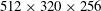 $512\times 320\times 256$
cells and is stretched in the normal direction by the tangent hyperbolical function (Vreman Reference Vreman2014). The grid points
$512\times 320\times 256$
cells and is stretched in the normal direction by the tangent hyperbolical function (Vreman Reference Vreman2014). The grid points
 $x_{2,j}$
of the cell centres are located at
$x_{2,j}$
of the cell centres are located at
 $$\begin{eqnarray}x_{2,j}=H\left(1+\frac{\text{tanh}(1.65(-1+2(j-{\textstyle \frac{1}{2}})/320))}{\text{tanh}(1.65)}\right),\quad j=1,2,\dots ,320.\end{eqnarray}$$
The uniform streamwise and spanwise grid spacings are equal to
 $7.5{\it\delta}_{{\it\nu}}$
and
$7.5{\it\delta}_{{\it\nu}}$
and
 $5.0{\it\delta}_{{\it\nu}}$
respectively. The grid spacing in the normal direction varies from
$5.0{\it\delta}_{{\it\nu}}$
respectively. The grid spacing in the normal direction varies from
 $0.99{\it\delta}_{{\it\nu}}$
at the wall to
$0.99{\it\delta}_{{\it\nu}}$
at the wall to
 $7{\it\delta}_{{\it\nu}}$
at the centre of the channel. These are standard grid sizes for DNS of single-phase channel flow (Moser, Kim & Mansour Reference Moser, Kim and Mansour1999) and are sufficiently small to compute mean velocity and Reynolds stress profiles accurately (Vreman & Kuerten Reference Vreman and Kuerten2014a
,Reference Vreman and Kuerten
b
).
$7{\it\delta}_{{\it\nu}}$
at the centre of the channel. These are standard grid sizes for DNS of single-phase channel flow (Moser, Kim & Mansour Reference Moser, Kim and Mansour1999) and are sufficiently small to compute mean velocity and Reynolds stress profiles accurately (Vreman & Kuerten Reference Vreman and Kuerten2014a
,Reference Vreman and Kuerten
b
).
The particles are tracked in a Lagrangian framework. The following equations are solved for each particle
 $p$
:
$p$
:
 $$\begin{eqnarray}\displaystyle & \displaystyle \frac{\text{d}\boldsymbol{x}^{p}}{\text{d}t}=\boldsymbol{v}^{p}, & \displaystyle\end{eqnarray}$$
 $$\begin{eqnarray}\displaystyle & \displaystyle m_{p}\frac{\text{d}\boldsymbol{v}^{p}}{\text{d}t}=\boldsymbol{F}_{coll}^{p}+\boldsymbol{F}^{p}+m_{p}g\boldsymbol{e}_{\mathbf{1}}, & \displaystyle\end{eqnarray}$$
 $$\begin{eqnarray}\displaystyle & \displaystyle I_{p}\frac{\text{d}{\bf\omega}^{p}}{\text{d}t}=\boldsymbol{T}_{coll}^{p}+\boldsymbol{T}^{p}. & \displaystyle\end{eqnarray}$$
 $p$
is written as a subscript, while in vector particle variables
$p$
is written as a subscript, while in vector particle variables
 $p$
is written as superscript.
$p$
is written as superscript.
The particle position, velocity and angular velocity are respectively denoted by
 $\boldsymbol{x}^{p}$
,
$\boldsymbol{x}^{p}$
,
 $\boldsymbol{v}^{p}$
and
$\boldsymbol{v}^{p}$
and
 ${\bf\omega}^{p}$
, while
${\bf\omega}^{p}$
, while
 $m_{p}={\rm\pi}{\it\rho}_{p}d_{p}^{3}/6$
is the mass of the particle and
$m_{p}={\rm\pi}{\it\rho}_{p}d_{p}^{3}/6$
is the mass of the particle and
 $I_{p}=(m_{p}d_{p}^{2})/10$
is the moment of inertia of the particle. The force and torque caused by the inter-particle collisions and particle–wall collisions on particle
$I_{p}=(m_{p}d_{p}^{2})/10$
is the moment of inertia of the particle. The force and torque caused by the inter-particle collisions and particle–wall collisions on particle
 $p$
at time
$p$
at time
 $t$
are represented by
$t$
are represented by
 $\boldsymbol{F}_{coll}^{p}$
and
$\boldsymbol{F}_{coll}^{p}$
and
 $\boldsymbol{T}_{coll}^{p}$
, while the force and torque exerted by the gas on the particle are represented by
$\boldsymbol{T}_{coll}^{p}$
, while the force and torque exerted by the gas on the particle are represented by
 $\boldsymbol{F}^{p}$
and
$\boldsymbol{F}^{p}$
and
 $\boldsymbol{T}^{p}$
. These forces and torques will be defined in later subsections.
$\boldsymbol{T}^{p}$
. These forces and torques will be defined in later subsections.
The time integration of the particle position and velocity is performed with forward Euler with (at least) three time steps per time step
 ${\rm\Delta}t$
of the Runge–Kutta method used for the gas phase. The forward Euler method has been selected because the time step is not the same for each particle, due to collisions. Since there are many collisions per time step, it is not efficient to update all particles after each collision. The time levels after stages 1, 2 and 3 of the Runge–Kutta method are
${\rm\Delta}t$
of the Runge–Kutta method used for the gas phase. The forward Euler method has been selected because the time step is not the same for each particle, due to collisions. Since there are many collisions per time step, it is not efficient to update all particles after each collision. The time levels after stages 1, 2 and 3 of the Runge–Kutta method are
 $t+{\rm\Delta}t/3$
,
$t+{\rm\Delta}t/3$
,
 $t+{\rm\Delta}t/2$
and
$t+{\rm\Delta}t/2$
and
 $t+{\rm\Delta}t$
respectively. The basic particle time step,
$t+{\rm\Delta}t$
respectively. The basic particle time step,
 ${\rm\Delta}t_{p}$
, is set to
${\rm\Delta}t_{p}$
, is set to
 ${\rm\Delta}t/3$
in stage 1,
${\rm\Delta}t/3$
in stage 1,
 ${\rm\Delta}t/6$
in stage 2 and
${\rm\Delta}t/6$
in stage 2 and
 ${\rm\Delta}t/2$
in stage 3. For particles that experience one or more collisions within
${\rm\Delta}t/2$
in stage 3. For particles that experience one or more collisions within
 ${\rm\Delta}t_{p}$
, the time integration over
${\rm\Delta}t_{p}$
, the time integration over
 ${\rm\Delta}t_{p}$
is divided into two or more substeps.
${\rm\Delta}t_{p}$
is divided into two or more substeps.
The feedback force at location
 $\boldsymbol{x}$
and time
$\boldsymbol{x}$
and time
 $t$
is defined by
$t$
is defined by
 $$\begin{eqnarray}\boldsymbol{f}(\boldsymbol{x},t)=\frac{1}{{\it\rho}}\mathop{\sum }_{p}\boldsymbol{F}^{p}(t){\it\delta}_{x}(\boldsymbol{x}-\boldsymbol{x}^{p}),\end{eqnarray}$$
where the
 ${\it\delta}_{x}$
is the delta function with unit
${\it\delta}_{x}$
is the delta function with unit
 $\text{m}^{-3}$
. The discretization of this equation is
$\text{m}^{-3}$
. The discretization of this equation is
 $$\begin{eqnarray}\boldsymbol{f}(\boldsymbol{x},t)=\frac{1}{{\it\rho}|V_{\boldsymbol{x}}|}\mathop{\sum }_{p}w_{p}(\boldsymbol{x},t)\boldsymbol{F}^{p}(t),\end{eqnarray}$$
where
 $|V_{\boldsymbol{x}}|$
is the volume of the Eulerian (gas phase) grid cell
$|V_{\boldsymbol{x}}|$
is the volume of the Eulerian (gas phase) grid cell
 $V_{\boldsymbol{x}}$
around
$V_{\boldsymbol{x}}$
around
 $\boldsymbol{x}$
, and the coefficients
$\boldsymbol{x}$
, and the coefficients
 $w_{p}(\boldsymbol{x},t)$
represent the force distribution coefficients. The simplest way is to define
$w_{p}(\boldsymbol{x},t)$
represent the force distribution coefficients. The simplest way is to define
 $w_{p}(\boldsymbol{x},t)=1$
if the particle location
$w_{p}(\boldsymbol{x},t)=1$
if the particle location
 $\boldsymbol{x}^{p}(t)$
is inside
$\boldsymbol{x}^{p}(t)$
is inside
 $V_{\boldsymbol{x}}$
and
$V_{\boldsymbol{x}}$
and
 $w_{p}(\boldsymbol{x},t)=0$
otherwise. However, we use a slightly different approach, which is more accurate and also more convenient on a staggered grid. In this approach the three gas velocity components are transferred from staggered to cell-centre positions (the cell centre is the position where also the pressure and the velocity divergence of the grid are defined). Then the gas velocity in
$w_{p}(\boldsymbol{x},t)=0$
otherwise. However, we use a slightly different approach, which is more accurate and also more convenient on a staggered grid. In this approach the three gas velocity components are transferred from staggered to cell-centre positions (the cell centre is the position where also the pressure and the velocity divergence of the grid are defined). Then the gas velocity in
 $\boldsymbol{x}^{p}$
is defined by linear interpolation of the cell-centre gas velocity to particle locations (particle centres). Then the particle forces
$\boldsymbol{x}^{p}$
is defined by linear interpolation of the cell-centre gas velocity to particle locations (particle centres). Then the particle forces
 $\boldsymbol{F}^{p}$
are computed. The weights of the linear interpolation just mentioned are reused to distribute the particle force, which is defined at the particle centre, to the eight surrounding cell-centre positions. Finally, the force
$\boldsymbol{F}^{p}$
are computed. The weights of the linear interpolation just mentioned are reused to distribute the particle force, which is defined at the particle centre, to the eight surrounding cell-centre positions. Finally, the force
 $\boldsymbol{f}$
is transferred to the staggered positions at cell faces by taking the average over the appropriate two cells for each component. No special treatment is used in the wall proximity. There, the cell size spacing in the normal direction is approximately two times smaller than the particle size, but the effective volume of fluid over which a particle force is distributed is still considerably larger than the particle volume. At the wall, the Eulerian cell volume
$\boldsymbol{f}$
is transferred to the staggered positions at cell faces by taking the average over the appropriate two cells for each component. No special treatment is used in the wall proximity. There, the cell size spacing in the normal direction is approximately two times smaller than the particle size, but the effective volume of fluid over which a particle force is distributed is still considerably larger than the particle volume. At the wall, the Eulerian cell volume
 $|V_{x}|$
is equal to 6.3 particle volumes. Due to the averaging of
$|V_{x}|$
is equal to 6.3 particle volumes. Due to the averaging of
 $\boldsymbol{f}$
to the staggered positions, the particle force is distributed over at least
$\boldsymbol{f}$
to the staggered positions, the particle force is distributed over at least
 $2|V_{x}|$
. At least, because due to the use of weight coefficients
$2|V_{x}|$
. At least, because due to the use of weight coefficients
 $w_{p}$
in (2.7), the effective fluid volume over which each particle force is distributed is generally larger than
$w_{p}$
in (2.7), the effective fluid volume over which each particle force is distributed is generally larger than
 $2|V_{x}|$
.
$2|V_{x}|$
.
The unladen case A0 is initialized by a parabolic mean profile with a suitable divergence-free perturbation. The particle-laden cases A1–A3 are initialized by a snapshot of the turbulent velocity field of case A0. Statistical averaging is started only after transient effects have disappeared. In each case the statistical averaging time is at least 0.5 s, which corresponds to 38 flow-through times, with the flow-through time defined by the streamwise channel length divided by the gas bulk velocity. Each particle-laden case contains 116 756 particles.
2.4. Particle–gas forces
The force
 $\boldsymbol{F}^{p}$
, exerted by the gas on a single free particle, is parametrized by the well-known Schiller–Naumann standard drag correlation:
$\boldsymbol{F}^{p}$
, exerted by the gas on a single free particle, is parametrized by the well-known Schiller–Naumann standard drag correlation:
 $$\begin{eqnarray}\boldsymbol{F}^{p}=\frac{m_{p}}{{\it\tau}_{p}}(1+0.15Re_{p}^{0.687})(\boldsymbol{u}-\boldsymbol{v}^{p}),\end{eqnarray}$$
where
 $Re_{p}$
is the Reynolds number of the particle, defined by
$Re_{p}$
is the Reynolds number of the particle, defined by
 $d_{p}|\boldsymbol{u}-\boldsymbol{v}^{p}|/{\it\nu}$
. Based upon recent literature on the relevance of the lift force (Zeng et al.
Reference Zeng, Balachandar, Fischer and Najjar2008), the inertial, added mass and history force (Armenio & Fiorotto Reference Armenio and Fiorotto2001; Bagchi & Balachandar Reference Bagchi and Balachandar2003; Burton & Eaton Reference Burton and Eaton2005), and hydrodynamic particle–particle interactions (Vreman Reference Vreman2007; Nasr et al.
Reference Nasr, Ahmadi and McLaughlin2009), explicit models for these forces are not included. In one-way coupled simulations of similar case, Rouson & Eaton (Reference Rouson and Eaton2001) tested the lift force expression derived by McLaughlin (Reference McLaughlin1993) and found that the term is negligible compared with the particle drag in the same direction. Fully resolved simulations of a single small particle in isotropic turbulence (Bagchi & Balachandar Reference Bagchi and Balachandar2003; Burton & Eaton Reference Burton and Eaton2005) and in wall-bounded turbulence (Zeng et al.
Reference Zeng, Balachandar, Fischer and Najjar2008) indicate that the standard drag law provides a good description for the mean force on the particle. However, these references also show that the error in the fluctuating force may be large and that incorporation of other terms of the Maxey Riley equation is no remedy for this limitation. A simulation method that fully resolves the boundary layers around the particles would of course be a more accurate method to simulate the turbulence modification. However, such a simulation is not possible yet for the present case, in which the flow domain contains more than
$d_{p}|\boldsymbol{u}-\boldsymbol{v}^{p}|/{\it\nu}$
. Based upon recent literature on the relevance of the lift force (Zeng et al.
Reference Zeng, Balachandar, Fischer and Najjar2008), the inertial, added mass and history force (Armenio & Fiorotto Reference Armenio and Fiorotto2001; Bagchi & Balachandar Reference Bagchi and Balachandar2003; Burton & Eaton Reference Burton and Eaton2005), and hydrodynamic particle–particle interactions (Vreman Reference Vreman2007; Nasr et al.
Reference Nasr, Ahmadi and McLaughlin2009), explicit models for these forces are not included. In one-way coupled simulations of similar case, Rouson & Eaton (Reference Rouson and Eaton2001) tested the lift force expression derived by McLaughlin (Reference McLaughlin1993) and found that the term is negligible compared with the particle drag in the same direction. Fully resolved simulations of a single small particle in isotropic turbulence (Bagchi & Balachandar Reference Bagchi and Balachandar2003; Burton & Eaton Reference Burton and Eaton2005) and in wall-bounded turbulence (Zeng et al.
Reference Zeng, Balachandar, Fischer and Najjar2008) indicate that the standard drag law provides a good description for the mean force on the particle. However, these references also show that the error in the fluctuating force may be large and that incorporation of other terms of the Maxey Riley equation is no remedy for this limitation. A simulation method that fully resolves the boundary layers around the particles would of course be a more accurate method to simulate the turbulence modification. However, such a simulation is not possible yet for the present case, in which the flow domain contains more than
 $10^{5}$
small moving particles.
$10^{5}$
small moving particles.
The particle angular velocity
 ${\bf\omega}^{p}$
is included in the PP-DNS, since it is required to describe non-ideal collisions, in particular collisions with non-zero tangential friction. The particle angular velocity is both generated and dissipated by non-ideal collisions via
${\bf\omega}^{p}$
is included in the PP-DNS, since it is required to describe non-ideal collisions, in particular collisions with non-zero tangential friction. The particle angular velocity is both generated and dissipated by non-ideal collisions via
 $\boldsymbol{T}^{p,c}$
. In addition, the particle angular velocity is influenced by the particle drag torque
$\boldsymbol{T}^{p,c}$
. In addition, the particle angular velocity is influenced by the particle drag torque
 $\boldsymbol{T}^{p}$
. The drag torque is included, because it was found to dampen the particle angular velocity fluctuation considerably. The drag torque is modelled by (Takagi Reference Takagi1977; Dennis, Singh & Ingham Reference Dennis, Singh and Ingham1980; Yamamoto et al.
Reference Yamamoto, Potthoff, Tanaka, Kajishima and Tsuji2001)
$\boldsymbol{T}^{p}$
. The drag torque is included, because it was found to dampen the particle angular velocity fluctuation considerably. The drag torque is modelled by (Takagi Reference Takagi1977; Dennis, Singh & Ingham Reference Dennis, Singh and Ingham1980; Yamamoto et al.
Reference Yamamoto, Potthoff, Tanaka, Kajishima and Tsuji2001)
 $$\begin{eqnarray}\boldsymbol{T}^{p}=-{\textstyle \frac{1}{2}}{\it\rho}(C_{1}Re_{p,a}^{-1/2}+C_{2}Re_{p,a}^{-1}+C_{3}Re_{p,a})({\textstyle \frac{1}{2}}d_{p})^{5}|{\bf\zeta}^{p}|{\bf\zeta}^{p}.\end{eqnarray}$$
In this equation
 ${\bf\zeta}^{p}={\bf\omega}^{p}-(\boldsymbol{{\rm\nabla}}\times \boldsymbol{u})/2$
and
${\bf\zeta}^{p}={\bf\omega}^{p}-(\boldsymbol{{\rm\nabla}}\times \boldsymbol{u})/2$
and
 $Re_{p,a}=d_{p}^{2}|{\bf\zeta}^{p}|/4{\it\nu}$
is the particle Reynolds number based on the angular velocity difference. The torque coefficients
$Re_{p,a}=d_{p}^{2}|{\bf\zeta}^{p}|/4{\it\nu}$
is the particle Reynolds number based on the angular velocity difference. The torque coefficients
 $(C_{1},C_{2},C_{3})$
are given by (0, 50.27, 0) if
$(C_{1},C_{2},C_{3})$
are given by (0, 50.27, 0) if
 $Re_{p,a}<1$
, (0, 50.27, 0.0418) if
$Re_{p,a}<1$
, (0, 50.27, 0.0418) if
 $1<Re_{p,a}<10$
, (5.32, 37.2, 5.32) if
$1<Re_{p,a}<10$
, (5.32, 37.2, 5.32) if
 $10<Re_{p,a}<20$
, (6.44, 32.2, 6.44) if
$10<Re_{p,a}<20$
, (6.44, 32.2, 6.44) if
 $20<Re_{p,a}<50$
and (6.45, 32.1, 6.45) if
$20<Re_{p,a}<50$
and (6.45, 32.1, 6.45) if
 $Re_{p,a}>50$
.
$Re_{p,a}>50$
.
2.5. Particle collisions
Although the volume fraction of the particle-laden simulations is only of the order of
 $10^{-4}$
, all collisions between particles are taken into account. It is often mentioned that inter-particle collisions are negligible if the volume fraction is smaller than
$10^{-4}$
, all collisions between particles are taken into account. It is often mentioned that inter-particle collisions are negligible if the volume fraction is smaller than
 $10^{-3}$
. This may be the case in isotropic turbulence; for wall-bounded turbulence it has repeatedly been shown that collisions do significantly influence the results if the volume fraction is of the order of
$10^{-3}$
. This may be the case in isotropic turbulence; for wall-bounded turbulence it has repeatedly been shown that collisions do significantly influence the results if the volume fraction is of the order of
 $10^{-4}$
or even lower (Li et al.
Reference Li, McLaughlin, Kontomaris and Portela2001; Yamamoto et al.
Reference Yamamoto, Potthoff, Tanaka, Kajishima and Tsuji2001; Vreman Reference Vreman2007; Nasr et al.
Reference Nasr, Ahmadi and McLaughlin2009). These references show that collisions reduce the tendency of preferential concentration of particles. Without collisions all particles slowly accumulate either at the walls or at the centre (Rouson & Eaton Reference Rouson and Eaton2001), while with collisions a statistically stationary steady state can be achieved.
$10^{-4}$
or even lower (Li et al.
Reference Li, McLaughlin, Kontomaris and Portela2001; Yamamoto et al.
Reference Yamamoto, Potthoff, Tanaka, Kajishima and Tsuji2001; Vreman Reference Vreman2007; Nasr et al.
Reference Nasr, Ahmadi and McLaughlin2009). These references show that collisions reduce the tendency of preferential concentration of particles. Without collisions all particles slowly accumulate either at the walls or at the centre (Rouson & Eaton Reference Rouson and Eaton2001), while with collisions a statistically stationary steady state can be achieved.
The particle collisions are modelled with a hard-sphere collision model. The normal restitution coefficient is given by
 $e_{r}=0.95$
and the tangential friction coefficient by
$e_{r}=0.95$
and the tangential friction coefficient by
 ${\it\mu}=0.3$
, which are the same values as in Yamamoto et al. (Reference Yamamoto, Potthoff, Tanaka, Kajishima and Tsuji2001). The tangential restitution coefficient is given by
${\it\mu}=0.3$
, which are the same values as in Yamamoto et al. (Reference Yamamoto, Potthoff, Tanaka, Kajishima and Tsuji2001). The tangential restitution coefficient is given by
 ${\it\beta}_{0}=0.33$
(Hoomans Reference Hoomans1999). Two particles
${\it\beta}_{0}=0.33$
(Hoomans Reference Hoomans1999). Two particles
 $p$
and
$p$
and
 $q$
collide when the distance between their point-particle locations is equal to
$q$
collide when the distance between their point-particle locations is equal to
 $(d_{p}+d_{q})/2$
. Conservation of momentum and angular momentum during collision between two particles
$(d_{p}+d_{q})/2$
. Conservation of momentum and angular momentum during collision between two particles
 $p$
and
$p$
and
 $q$
implies the following modification of the particle velocity and angular velocity (Hoomans et al.
Reference Hoomans, Kuipers, Briels and van Swaaij1996; Hoomans Reference Hoomans1999):
$q$
implies the following modification of the particle velocity and angular velocity (Hoomans et al.
Reference Hoomans, Kuipers, Briels and van Swaaij1996; Hoomans Reference Hoomans1999):
 $$\begin{eqnarray}\displaystyle & \boldsymbol{v}^{p}=\boldsymbol{v}^{p,0}+\boldsymbol{J}/m_{p}, & \displaystyle\end{eqnarray}$$
 $$\begin{eqnarray}\displaystyle & \boldsymbol{v}^{q}=\boldsymbol{v}^{q,0}-\boldsymbol{J}/m_{q}, & \displaystyle\end{eqnarray}$$
 $$\begin{eqnarray}\displaystyle & \displaystyle {\bf\omega}^{p}={\bf\omega}^{p,0}-\frac{d_{p}}{2I_{p}}\boldsymbol{n}\times \boldsymbol{J}, & \displaystyle\end{eqnarray}$$
 $$\begin{eqnarray}\displaystyle & \displaystyle {\bf\omega}^{q}={\bf\omega}^{q,0}-\frac{d_{q}}{2I_{q}}\boldsymbol{n}\times \boldsymbol{J}, & \displaystyle\end{eqnarray}$$
 $\boldsymbol{n}$
is defined by
$\boldsymbol{n}$
is defined by
 $(\boldsymbol{x}^{p}-\boldsymbol{x}^{q})/|\boldsymbol{x}^{p}-\boldsymbol{x}^{q}|$
. The relative velocity vector before collision is defined by
$(\boldsymbol{x}^{p}-\boldsymbol{x}^{q})/|\boldsymbol{x}^{p}-\boldsymbol{x}^{q}|$
. The relative velocity vector before collision is defined by  $$\begin{eqnarray}\boldsymbol{v}^{pq,0}=(\boldsymbol{v}^{p,0}-{\textstyle \frac{1}{2}}d_{p}{\bf\omega}^{p,0}\times \boldsymbol{n})-(\boldsymbol{v}^{q,0}+{\textstyle \frac{1}{2}}d_{q}{\bf\omega}^{q,0}\times \boldsymbol{n}),\end{eqnarray}$$
with normal component
 $v_{n}=\boldsymbol{v}^{pq,0}\boldsymbol{\cdot }\boldsymbol{n}$
. The tangential unit vector
$v_{n}=\boldsymbol{v}^{pq,0}\boldsymbol{\cdot }\boldsymbol{n}$
. The tangential unit vector
 $\boldsymbol{t}$
is defined by
$\boldsymbol{t}$
is defined by
 $(\boldsymbol{v}^{pq,0}-v_{n}\boldsymbol{n})/|\boldsymbol{v}^{pq,0}-v_{n}\boldsymbol{n}|$
. The impulse vector
$(\boldsymbol{v}^{pq,0}-v_{n}\boldsymbol{n})/|\boldsymbol{v}^{pq,0}-v_{n}\boldsymbol{n}|$
. The impulse vector
 $\boldsymbol{J}$
is then defined as
$\boldsymbol{J}$
is then defined as
 $\boldsymbol{J}=J_{n}\boldsymbol{n}+J_{t}\boldsymbol{t}$
, where the normal component
$\boldsymbol{J}=J_{n}\boldsymbol{n}+J_{t}\boldsymbol{t}$
, where the normal component
 $J_{n}$
is given by
$J_{n}$
is given by
 $-(1+e_{r})v_{n}/B_{2}$
and
$-(1+e_{r})v_{n}/B_{2}$
and
 $B_{2}=1/m_{p}+1/m_{q}$
. The tangential component
$B_{2}=1/m_{p}+1/m_{q}$
. The tangential component
 $J_{t}$
depends on the maximum Coulomb friction
$J_{t}$
depends on the maximum Coulomb friction
 ${\it\mu}J_{n}$
and
${\it\mu}J_{n}$
and
 $J_{{\it\beta}}=(1+{\it\beta}_{0})(\boldsymbol{v}^{pq,0}\boldsymbol{\cdot }\boldsymbol{t})/B_{1}$
with
$J_{{\it\beta}}=(1+{\it\beta}_{0})(\boldsymbol{v}^{pq,0}\boldsymbol{\cdot }\boldsymbol{t})/B_{1}$
with
 $B_{1}=7B_{2}/2$
. It can be proven that at contact
$B_{1}=7B_{2}/2$
. It can be proven that at contact
 ${\it\mu}J_{n}\geqslant 0$
and
${\it\mu}J_{n}\geqslant 0$
and
 $J_{{\it\beta}}\geqslant 0$
. If
$J_{{\it\beta}}\geqslant 0$
. If
 $J_{{\it\beta}}\leqslant {\it\mu}J_{n}$
, the collision is of the sticking type and
$J_{{\it\beta}}\leqslant {\it\mu}J_{n}$
, the collision is of the sticking type and
 $J_{t}=-J_{{\it\beta}}$
. However, if
$J_{t}=-J_{{\it\beta}}$
. However, if
 $J_{{\it\beta}}>{\it\mu}J_{n}$
, the collision is of the sliding type and
$J_{{\it\beta}}>{\it\mu}J_{n}$
, the collision is of the sliding type and
 $J_{t}=-{\it\mu}J_{n}$
(Hoomans et al.
Reference Hoomans, Kuipers, Briels and van Swaaij1996; Hoomans Reference Hoomans1999). Since (2.13) with a plus instead of a minus sign was also encountered in the literature, it is stressed that both minus signs in (2.12) and (2.13) are correct. This directly follows from the conservation of angular momentum about the centre of mass of the two particles during a collision.
$J_{t}=-{\it\mu}J_{n}$
(Hoomans et al.
Reference Hoomans, Kuipers, Briels and van Swaaij1996; Hoomans Reference Hoomans1999). Since (2.13) with a plus instead of a minus sign was also encountered in the literature, it is stressed that both minus signs in (2.12) and (2.13) are correct. This directly follows from the conservation of angular momentum about the centre of mass of the two particles during a collision.
If particle
 $p$
is involved in collision
$p$
is involved in collision
 $k$
, we define
$k$
, we define
 $\boldsymbol{J}^{p,k}=m_{p}(\boldsymbol{v}^{p}-\boldsymbol{v}^{p,0})$
, where
$\boldsymbol{J}^{p,k}=m_{p}(\boldsymbol{v}^{p}-\boldsymbol{v}^{p,0})$
, where
 $\boldsymbol{v}^{p}$
is the post- and
$\boldsymbol{v}^{p}$
is the post- and
 $\boldsymbol{v}^{p,0}$
the pre-collision velocity of particle
$\boldsymbol{v}^{p,0}$
the pre-collision velocity of particle
 $p$
at collision
$p$
at collision
 $k$
. Thus, for the particles
$k$
. Thus, for the particles
 $p$
and
$p$
and
 $q$
involved in collision
$q$
involved in collision
 $k$
, we have
$k$
, we have
 $\boldsymbol{J}^{q,k}=-\boldsymbol{J}^{p,k}=-\boldsymbol{J}$
. For any particle
$\boldsymbol{J}^{q,k}=-\boldsymbol{J}^{p,k}=-\boldsymbol{J}$
. For any particle
 $p$
not involved in collision
$p$
not involved in collision
 $k$
,
$k$
,
 $\boldsymbol{J}^{p,k}=0$
. If particle
$\boldsymbol{J}^{p,k}=0$
. If particle
 $p$
collides with a plane wall in the
$p$
collides with a plane wall in the
 $x_{2}$
direction, then the relative velocity vector is aligned with the
$x_{2}$
direction, then the relative velocity vector is aligned with the
 $x_{2}$
direction. The equations for a particle–wall collision can be derived from those of a particle–particle collision in the limit
$x_{2}$
direction. The equations for a particle–wall collision can be derived from those of a particle–particle collision in the limit
 $d_{q}\rightarrow \infty$
and
$d_{q}\rightarrow \infty$
and
 $m_{q}\rightarrow \infty$
.
$m_{q}\rightarrow \infty$
.
The collision force and torque vectors,
 $\boldsymbol{F}_{coll}^{p}$
and
$\boldsymbol{F}_{coll}^{p}$
and
 $\boldsymbol{T}_{coll}^{p}$
, can be expressed as a sum of temporal delta functions, one delta function for each collision,
$\boldsymbol{T}_{coll}^{p}$
, can be expressed as a sum of temporal delta functions, one delta function for each collision,
 $$\begin{eqnarray}\displaystyle & \boldsymbol{F}_{coll}^{p}=\displaystyle \mathop{\sum }_{k}\boldsymbol{J}^{p,k}{\it\delta}_{t}(t-t_{coll,k}), & \displaystyle\end{eqnarray}$$
 $$\begin{eqnarray}\displaystyle & \boldsymbol{T}_{coll}^{p}=\displaystyle -\frac{1}{2}d_{p}\mathop{\sum }_{k}(\boldsymbol{n}^{k}\times \boldsymbol{J}^{k}){\it\delta}_{t}(t-t_{coll,k}), & \displaystyle\end{eqnarray}$$
 $k$
is the index that runs over all collisions (note that
$k$
is the index that runs over all collisions (note that
 $\boldsymbol{J}^{p,k}=0$
for any particle
$\boldsymbol{J}^{p,k}=0$
for any particle
 $p$
not involved in collision
$p$
not involved in collision
 $k$
). The time of collision
$k$
). The time of collision
 $k$
is denoted by
$k$
is denoted by
 $t_{coll,k}$
. The unit of the delta function
$t_{coll,k}$
. The unit of the delta function
 ${\it\delta}_{t}$
is
${\it\delta}_{t}$
is
 $\text{s}^{-1}$
. If the collisions were ideal,
$\text{s}^{-1}$
. If the collisions were ideal,
 $e_{r}$
would be 1 and
$e_{r}$
would be 1 and
 ${\it\beta}_{0}$
would be
${\it\beta}_{0}$
would be
 $-1$
, then
$-1$
, then
 $J_{t}$
,
$J_{t}$
,
 $\boldsymbol{n}\times \boldsymbol{J}$
and
$\boldsymbol{n}\times \boldsymbol{J}$
and
 $\boldsymbol{T}_{coll}^{p}$
would be zero. If in addition the rotational drag force were neglected, the angular particle velocities would remain constant in time and there would be no need to include them in the simulation.
$\boldsymbol{T}_{coll}^{p}$
would be zero. If in addition the rotational drag force were neglected, the angular particle velocities would remain constant in time and there would be no need to include them in the simulation.
An efficient search for collision partners is facilitated by a uniform secondary grid (
 $120\times 40\times 40$
cells). Each cell of this secondary grid has a list attached that contains the particle indices for the particles located in that cell. Collisions that involve a free particle in a certain cell of the particle grid are detected by checking all particles in the neighbouring cells. The lists are set up before each particle time step and updated after each collision. To ensure that no collision is missed, the absolute velocity of each particle is verified to remain smaller than the size of the particle grid cells divided by twice the basic particle time step. In addition, for each collision it is verified that the particle involved touches the other particle (or the wall) without any overlap.
$120\times 40\times 40$
cells). Each cell of this secondary grid has a list attached that contains the particle indices for the particles located in that cell. Collisions that involve a free particle in a certain cell of the particle grid are detected by checking all particles in the neighbouring cells. The lists are set up before each particle time step and updated after each collision. To ensure that no collision is missed, the absolute velocity of each particle is verified to remain smaller than the size of the particle grid cells divided by twice the basic particle time step. In addition, for each collision it is verified that the particle involved touches the other particle (or the wall) without any overlap.
2.6. Forcing of the flow
Before we describe the forcing technique, the two averaging operators used in this paper are defined. The statistical mean of a quantity
 $Q$
is defined by
$Q$
is defined by
 $$\begin{eqnarray}\overline{Q}(x_{2})=\frac{1}{2(t_{2}-t_{1})}\int _{t_{1}}^{t_{2}}\int _{0}^{L_{1}}\int _{0}^{L_{3}}(Q(x_{1},x_{2},x_{3},t)+c_{Q}Q(x_{1},L_{2}-x_{2},x_{3},t))\,\text{d}x_{3}\,\text{d}x_{1}\,\text{d}t,\end{eqnarray}$$
where
 $t_{1}$
and
$t_{1}$
and
 $t_{2}$
are two times, such that (theoretically)
$t_{2}$
are two times, such that (theoretically)
 $t_{2}-t_{1}\rightarrow \infty$
. To increase the statistical sample size in practice, both halves of the channel are included in the average, using a parity coefficient
$t_{2}-t_{1}\rightarrow \infty$
. To increase the statistical sample size in practice, both halves of the channel are included in the average, using a parity coefficient
 $c_{Q}$
, equal to 1 for even and
$c_{Q}$
, equal to 1 for even and
 $-1$
for odd statistical quantities. Thus,
$-1$
for odd statistical quantities. Thus,
 $c_{Q}=1$
in the computation of, for example,
$c_{Q}=1$
in the computation of, for example,
 $\overline{u}_{1}$
,
$\overline{u}_{1}$
,
 $\overline{u}_{3}$
,
$\overline{u}_{3}$
,
 $\overline{u_{1}^{2}}$
,
$\overline{u_{1}^{2}}$
,
 $\overline{u_{2}^{2}}$
,
$\overline{u_{2}^{2}}$
,
 $\overline{u_{3}^{2}}$
,
$\overline{u_{3}^{2}}$
,
 $\overline{\partial u_{2}/\partial x_{2}}$
,
$\overline{\partial u_{2}/\partial x_{2}}$
,
 $\overline{f_{1}}$
,
$\overline{f_{1}}$
,
 $\overline{u_{2}f_{2}}$
, while
$\overline{u_{2}f_{2}}$
, while
 $c_{Q}=-1$
in the computation of, for example,
$c_{Q}=-1$
in the computation of, for example,
 $\overline{u}_{2}$
,
$\overline{u}_{2}$
,
 $\overline{u_{1}u_{2}}$
,
$\overline{u_{1}u_{2}}$
,
 $\overline{\partial u_{1}/\partial x_{2}}$
,
$\overline{\partial u_{1}/\partial x_{2}}$
,
 $\overline{f_{2}}$
. The ensemble average of particle properties, also denoted with an overbar, is similarly defined, except that the integrals over the
$\overline{f_{2}}$
. The ensemble average of particle properties, also denoted with an overbar, is similarly defined, except that the integrals over the
 $x_{1}{-}x_{3}$
planes are replaced by averages over all particles in (or near) these planes. The fluctuation of a quantity is defined by
$x_{1}{-}x_{3}$
planes are replaced by averages over all particles in (or near) these planes. The fluctuation of a quantity is defined by
 $Q^{\prime }=Q-\overline{Q}$
. In addition, we introduce the domain average of a quantity
$Q^{\prime }=Q-\overline{Q}$
. In addition, we introduce the domain average of a quantity
 $Q$
:
$Q$
:
 $$\begin{eqnarray}\langle Q\rangle (t)=\frac{1}{L_{1}L_{2}L_{3}}\int _{0}^{L_{1}}\int _{0}^{L_{2}}\int _{0}^{L_{3}}Q(x_{1},x_{2},x_{3},t)\,\text{d}x_{3}\,\text{d}x_{2}\,\text{d}x_{1}.\end{eqnarray}$$
The domain average applied to a mean quantity,
 $\langle \overline{Q}\rangle$
, is the same as the mean quantity averaged over the
$\langle \overline{Q}\rangle$
, is the same as the mean quantity averaged over the
 $x_{2}$
direction and does not depend on
$x_{2}$
direction and does not depend on
 $t$
,
$t$
,
 $x_{1}$
,
$x_{1}$
,
 $x_{2}$
,
$x_{2}$
,
 $x_{3}$
.
$x_{3}$
.
The overall force balance of the flow is given by the sum of the domain-averaged mean gas and domain-averaged mean particle momentum equation in the streamwise direction:
 $$\begin{eqnarray}{\it\rho}(1+{\it\phi})g+{\it\rho}\overline{a}-{\it\rho}u_{{\it\tau}}^{2}/H+F_{wall}=0,\end{eqnarray}$$
where
 $u_{{\it\tau}}=({\it\nu}\,\text{d}\overline{u}/\text{d}x_{2})^{1/2}$
is the friction velocity. The term
$u_{{\it\tau}}=({\it\nu}\,\text{d}\overline{u}/\text{d}x_{2})^{1/2}$
is the friction velocity. The term
 $F_{wall}$
represents the streamwise force exerted by the walls on the particles per unit of volume,
$F_{wall}$
represents the streamwise force exerted by the walls on the particles per unit of volume,
 $$\begin{eqnarray}F_{wall}=\frac{1}{(t_{2}-t_{1})L_{1}L_{2}L_{3}}\int _{t_{1}}^{t_{2}}\mathop{\sum }_{p}F_{coll,1}^{p}\,\text{d}t,\end{eqnarray}$$
where the index
 $p$
runs over all free particles. If this index ran over the free particles that collide with the wall (or collide with fixed wall particles), then the force would be equal and opposite, since the sum over the forces of all collisions between free particles is zero (
$p$
runs over all free particles. If this index ran over the free particles that collide with the wall (or collide with fixed wall particles), then the force would be equal and opposite, since the sum over the forces of all collisions between free particles is zero (
 $\boldsymbol{J}^{q,k}=-\boldsymbol{J}^{p,k}$
).
$\boldsymbol{J}^{q,k}=-\boldsymbol{J}^{p,k}$
).
The overall balance, (2.19), shows that it is not easy to decide what should remain constant in a study where laden cases are compared with an unladen case. Suppose that the streamwise pressure gradient,
 ${\it\rho}\overline{a}$
, is held constant. Then an increase of
${\it\rho}\overline{a}$
, is held constant. Then an increase of
 ${\it\phi}$
necessarily implies an increase of the wall friction forces,
${\it\phi}$
necessarily implies an increase of the wall friction forces,
 ${\it\rho}u_{{\it\tau}}^{2}/H-F_{wall}$
, which means that the fluid friction velocity,
${\it\rho}u_{{\it\tau}}^{2}/H-F_{wall}$
, which means that the fluid friction velocity,
 $u_{{\it\tau}}$
, or the particle–wall friction force,
$u_{{\it\tau}}$
, or the particle–wall friction force,
 $-F_{wall}$
, increases. If the latter were negligible,
$-F_{wall}$
, increases. If the latter were negligible,
 $u_{{\it\tau}}$
at
$u_{{\it\tau}}$
at
 ${\it\phi}=0.8$
would become
${\it\phi}=0.8$
would become
 $1.8^{1/2}=1.34$
times larger than in the unladen case, i.e. the friction Reynolds number and probably also the bulk Reynolds number would become much larger, such that the grid would have to be finer than in the unladen case.
$1.8^{1/2}=1.34$
times larger than in the unladen case, i.e. the friction Reynolds number and probably also the bulk Reynolds number would become much larger, such that the grid would have to be finer than in the unladen case.
The literature on vertical particle-laden channel or pipe flows shows that, instead of the streamwise pressure gradient, another quantity is usually fixed in a comparison between laden and unladen cases. In the experiments of KFE1994, the mean centreline velocity of the gas was fixed, since the authors state on pp. 116–117: ‘for each set of particle conditions, the tunnel speed was adjusted so that the laden-flow velocity matched the unladen-flow velocity at the centreline’. In the simulations of Yamamoto et al. (Reference Yamamoto, Potthoff, Tanaka, Kajishima and Tsuji2001) the quantity
 $(1+{\it\phi})g+\overline{a}$
was fixed. In the simulations of Segura (Reference Segura2004) the bulk flow was apparently fixed, since the authors mention that the simulations were run at the same bulk Reynolds number. Mito & Hanratty (Reference Mito and Hanratty2006) explicitly mention that the bulk velocity was fixed. In the pipe flow experiments of Caraman et al. (Reference Caraman, Borée and Simonin2003) and Borée & Caraman (Reference Borée and Caraman2005) and corresponding simulations of Vreman (Reference Vreman2007), the bulk flow was fixed as well.
$(1+{\it\phi})g+\overline{a}$
was fixed. In the simulations of Segura (Reference Segura2004) the bulk flow was apparently fixed, since the authors mention that the simulations were run at the same bulk Reynolds number. Mito & Hanratty (Reference Mito and Hanratty2006) explicitly mention that the bulk velocity was fixed. In the pipe flow experiments of Caraman et al. (Reference Caraman, Borée and Simonin2003) and Borée & Caraman (Reference Borée and Caraman2005) and corresponding simulations of Vreman (Reference Vreman2007), the bulk flow was fixed as well.
In view of the above discussion of the literature, the present simulations are performed for a prescribed bulk velocity, which means that
 $a(t)$
is adapted at each time step to keep the domain-average velocity constant. The same bulk velocity is prescribed in each simulation case. Since the numerical scheme is fully explicit and conserves momentum, there is no need for a control algorithm;
$a(t)$
is adapted at each time step to keep the domain-average velocity constant. The same bulk velocity is prescribed in each simulation case. Since the numerical scheme is fully explicit and conserves momentum, there is no need for a control algorithm;
 $L_{1}L_{2}L_{3}(g+a(t))$
is set equal to the instantaneous viscous shear stress integrated over the walls minus the instantaneous streamwise feedback force integrated over the spatial domain. Forcing to maintain a constant volumetric flow rate is also a standard approach in DNS of unladen turbulent channel flows. Since the effects of the particles on the mean gas velocity are relatively small (see the next section), a comparison for constant bulk velocity can be expected to lead to the same conclusions as a comparison for constant centreline velocity.
$L_{1}L_{2}L_{3}(g+a(t))$
is set equal to the instantaneous viscous shear stress integrated over the walls minus the instantaneous streamwise feedback force integrated over the spatial domain. Forcing to maintain a constant volumetric flow rate is also a standard approach in DNS of unladen turbulent channel flows. Since the effects of the particles on the mean gas velocity are relatively small (see the next section), a comparison for constant bulk velocity can be expected to lead to the same conclusions as a comparison for constant centreline velocity.
2.7. Wall roughness
A rough wall is defined as a plane coated with tiny wall particles, half-spheres of diameter
 $d_{p,w}$
, with the circular side of each half-sphere fixed on the plane. The wall particles are arranged in square pitch of size
$d_{p,w}$
, with the circular side of each half-sphere fixed on the plane. The wall particles are arranged in square pitch of size
 $d_{p,w}$
; each wall particle touches four neighbouring wall particles, two of these neighbours are aligned in the
$d_{p,w}$
; each wall particle touches four neighbouring wall particles, two of these neighbours are aligned in the
 $x_{1}$
direction, the other two are aligned in the
$x_{1}$
direction, the other two are aligned in the
 $x_{3}$
direction. For this pattern, the standard deviation of the wall roughness
$x_{3}$
direction. For this pattern, the standard deviation of the wall roughness
 $k_{rms}$
is approximated by
$k_{rms}$
is approximated by
 $0.172d_{p,w}$
, while the peak-to-trough wall roughness
$0.172d_{p,w}$
, while the peak-to-trough wall roughness
 $k_{l}$
is equal to
$k_{l}$
is equal to
 $0.5d_{p,w}$
. The diameter
$0.5d_{p,w}$
. The diameter
 $d_{p,w}$
of the wall particles is smaller than the wall unit
$d_{p,w}$
of the wall particles is smaller than the wall unit
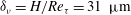 ${\it\delta}_{{\it\nu}}=H/Re_{{\it\tau}}=31~{\rm\mu}\text{m}$
:
${\it\delta}_{{\it\nu}}=H/Re_{{\it\tau}}=31~{\rm\mu}\text{m}$
:
 $d_{p,w}=10~{\rm\mu}\text{m}$
in case A2 and
$d_{p,w}=10~{\rm\mu}\text{m}$
in case A2 and
 $d_{p,w}=20~{\rm\mu}\text{m}$
in case A3. Thus,
$d_{p,w}=20~{\rm\mu}\text{m}$
in case A3. Thus,
 $k_{rms}^{+}=0.055$
and
$k_{rms}^{+}=0.055$
and
 $k_{l}^{+}=0.16$
in case A2, while
$k_{l}^{+}=0.16$
in case A2, while
 $k_{rms}^{+}=0.11$
and
$k_{rms}^{+}=0.11$
and
 $k_{l}^{+}=0.32$
in case A3. As discussed in the introduction, these values are sufficiently small to justify the application of smooth boundary conditions for the gas phase.
$k_{l}^{+}=0.32$
in case A3. As discussed in the introduction, these values are sufficiently small to justify the application of smooth boundary conditions for the gas phase.
The equations for a collision between a free particle
 $p$
and a wall particle
$p$
and a wall particle
 $q$
can be derived from the equations for a collision between two free particles by taking the limit
$q$
can be derived from the equations for a collision between two free particles by taking the limit
 $m_{q}\rightarrow \infty$
, such that
$m_{q}\rightarrow \infty$
, such that
 $\boldsymbol{v}^{q}$
and
$\boldsymbol{v}^{q}$
and
 ${\bf\omega}^{q}$
remain zero. There are a large number of wall particles in the rough cases (96 million in case A2, 24 million in case A3). Fortunately, due to the regular structure of the locations of these particles, it is not necessary to store the positions of all wall particles. In the simulations, wall-particle positions were stored for a square of
${\bf\omega}^{q}$
remain zero. There are a large number of wall particles in the rough cases (96 million in case A2, 24 million in case A3). Fortunately, due to the regular structure of the locations of these particles, it is not necessary to store the positions of all wall particles. In the simulations, wall-particle positions were stored for a square of
 $9~\text{mm}^{2}$
; from these positions the positions of the other wall particles were recomputed whenever they were required.
$9~\text{mm}^{2}$
; from these positions the positions of the other wall particles were recomputed whenever they were required.
In the present paper, a rough wall denotes a wall with a bumpy surface, while a smooth wall denotes a wall with a flat surface. In both the smooth and rough cases, the coefficient of friction
 ${\it\mu}$
is 0.3 for particle–particle and particle–wall collisions. Thus, the smooth wall is in fact a flat frictional wall (Jenkins & Louge Reference Jenkins and Louge1997). In addition, it is remarked that bumpiness in the form of spheres fixed to a plane is a well-known concept in granular flow experiments (Pouliquen Reference Pouliquen1999). In the granular flow literature, a so-called specularity coefficient has been used to describe phenomenologically the diffusive scatter of particles caused by bumpiness of the surface of the boundary (Johnson & Jackson Reference Johnson and Jackson1987).
${\it\mu}$
is 0.3 for particle–particle and particle–wall collisions. Thus, the smooth wall is in fact a flat frictional wall (Jenkins & Louge Reference Jenkins and Louge1997). In addition, it is remarked that bumpiness in the form of spheres fixed to a plane is a well-known concept in granular flow experiments (Pouliquen Reference Pouliquen1999). In the granular flow literature, a so-called specularity coefficient has been used to describe phenomenologically the diffusive scatter of particles caused by bumpiness of the surface of the boundary (Johnson & Jackson Reference Johnson and Jackson1987).
3. Point-particle DNS results
3.1. Velocity and volume fraction statistics
The basic characteristics of the mean velocity profiles and particle collision frequencies are shown in table 2. Columns two to six contain the gas friction velocity
 $u_{{\it\tau}}$
, gas bulk velocity
$u_{{\it\tau}}$
, gas bulk velocity
 $u_{b}=\langle \overline{u}_{1}\rangle$
, gas mean centreline velocity
$u_{b}=\langle \overline{u}_{1}\rangle$
, gas mean centreline velocity
 $u_{cl}$
, particle bulk velocity
$u_{cl}$
, particle bulk velocity
 $v_{b}=\langle \overline{v}_{1}\rangle$
and particle mean centreline velocity
$v_{b}=\langle \overline{v}_{1}\rangle$
and particle mean centreline velocity
 $v_{cl}$
. The last two columns contain the overall collision frequencies. A p–p collision is a collision between two free particles somewhere in the domain. A p–w collision is a collision between a free particle and a wall or, in the rough-wall cases, a particle fixed on a wall. We will refer to the values in the table during the discussion of figures 1–4. Like in KFE1994 and in the work of Benson et al. (Reference Benson, Tanaka and Eaton2005), the mean and fluctuation velocity profiles in the figures in this section have been normalized with the mean centreline velocity of the unladen case,
$v_{cl}$
. The last two columns contain the overall collision frequencies. A p–p collision is a collision between two free particles somewhere in the domain. A p–w collision is a collision between a free particle and a wall or, in the rough-wall cases, a particle fixed on a wall. We will refer to the values in the table during the discussion of figures 1–4. Like in KFE1994 and in the work of Benson et al. (Reference Benson, Tanaka and Eaton2005), the mean and fluctuation velocity profiles in the figures in this section have been normalized with the mean centreline velocity of the unladen case,
 $u_{cl,0}=10.42~\text{m}~\text{s}^{-1}$
. A typical run of a particle-laden case with rough walls, which was performed on an eight-core (16-thread) processor of a Linux cluster, took approximately two weeks (wall-clock time); roughly 50 % of that time was used by the particle collision module.
$u_{cl,0}=10.42~\text{m}~\text{s}^{-1}$
. A typical run of a particle-laden case with rough walls, which was performed on an eight-core (16-thread) processor of a Linux cluster, took approximately two weeks (wall-clock time); roughly 50 % of that time was used by the particle collision module.

Figure 1. Mean gas (a) and mean particle streamwise velocity profile (b), normalized with the unladen centreline velocity
 $u_{cl,0}$
. Unladen DNS A0 (dashed) and the laden simulations A1 (solid, no markers), A2 (solid, circles) and A3 (solid, triangles). The filled circles and filled triangles represent experiments of Kulick et al. (Reference Kulick, Fessler and Eaton1994) for copper particles at
$u_{cl,0}$
. Unladen DNS A0 (dashed) and the laden simulations A1 (solid, no markers), A2 (solid, circles) and A3 (solid, triangles). The filled circles and filled triangles represent experiments of Kulick et al. (Reference Kulick, Fessler and Eaton1994) for copper particles at
 ${\it\phi}=0.4$
and
${\it\phi}=0.4$
and
 ${\it\phi}=0.2$
respectively; the stars represent a fully rough experiment of Benson et al. (Reference Benson, Tanaka and Eaton2005) at
${\it\phi}=0.2$
respectively; the stars represent a fully rough experiment of Benson et al. (Reference Benson, Tanaka and Eaton2005) at
 ${\it\phi}=0.15$
. The unladen mean velocity profile is shown in both (a) and (b).
${\it\phi}=0.15$
. The unladen mean velocity profile is shown in both (a) and (b).
Table 2. Dimensional mean streamwise velocity and collision frequency characteristics in the unladen case, A0, and the three laden cases, A1 (smooth wall), A2 (rough wall,
 $d_{p,w}=10~{\rm\mu}\text{m}$
) and A3 (rough wall,
$d_{p,w}=10~{\rm\mu}\text{m}$
) and A3 (rough wall,
 $d_{p,w}=20~{\rm\mu}\text{m}$
).
$d_{p,w}=20~{\rm\mu}\text{m}$
).

The mean velocity profiles of the two phases are shown in figure 1. According to KFE1994 the mean gas velocity profile in the experiments was not significantly modified in the laden cases up to a mass loading ratio of 0.4. The experimental uncertainty in the mean gas-phase velocity profiles was reported to be approximately 2 %. The near-wall flow, including
 $u_{{\it\tau}}$
, could not be measured in the laden cases. In the present simulations, the effect of the particles on the mean gas velocity profile appears also to be small, in particular in case A2 (rough wall,
$u_{{\it\tau}}$
, could not be measured in the laden cases. In the present simulations, the effect of the particles on the mean gas velocity profile appears also to be small, in particular in case A2 (rough wall,
 $10~{\rm\mu}\text{m}$
); the mean gas velocity profiles of case A2 and the unladen case apparently coincide in figure 1(a). Quantitatively, the difference between the mean gas velocity profiles of A2 and A0 is less than 1 % for
$10~{\rm\mu}\text{m}$
); the mean gas velocity profiles of case A2 and the unladen case apparently coincide in figure 1(a). Quantitatively, the difference between the mean gas velocity profiles of A2 and A0 is less than 1 % for
 $u_{{\it\tau}}$
and
$u_{{\it\tau}}$
and
 $u_{cl}$
, while the maximum deviation, 2.6 %, is attained in the near-wall region (at
$u_{cl}$
, while the maximum deviation, 2.6 %, is attained in the near-wall region (at
 $y^{+}\approx 7$
). Figure 1(a) indicates that, compared with case A2, the particles in cases A1 and A3 have a slightly larger effect on the mean gas velocity profile, but quantitatively the effects are also small in these cases (see table 2).
$y^{+}\approx 7$
). Figure 1(a) indicates that, compared with case A2, the particles in cases A1 and A3 have a slightly larger effect on the mean gas velocity profile, but quantitatively the effects are also small in these cases (see table 2).
The mean particle velocity profile is flatter than the mean gas velocity profile in simulations A1–A3. An explanation of this feature of wall-bounded flows laden with heavy particles was already given in the introduction. The wall roughness is observed to lower and to flatten the mean particle velocity, like in experiments (Benson et al.
Reference Benson, Tanaka and Eaton2005). The mean particle velocity becomes lower because the rough wall causes more friction. The particle centreline velocity
 $v_{cl}$
is
$v_{cl}$
is
 $0.86u_{cl,0}$
in case A2 and
$0.86u_{cl,0}$
in case A2 and
 $0.70u_{cl,0}$
in case A3. The mean particle velocity becomes flatter due to stronger transverse mixing; the interaction of the particles with the rough wall enhances the wall-normal (transverse) particle velocity fluctuation in particular (Kussin & Sommerfeld Reference Kussin and Sommerfeld2002; Benson et al.
Reference Benson, Tanaka and Eaton2005; Squires & Simonin Reference Squires and Simonin2006; Vreman Reference Vreman2007; Breuer et al.
Reference Breuer, Alletto and Langfeldt2012), as will be shown in figure 3. The mean particle profiles in cases A2 and A3 are nearly horizontal, like the mean particle velocity profile measured in a fully rough channel (Benson et al.
Reference Benson, Tanaka and Eaton2005), shown in figure 1(b). In addition, two mean particle velocity profiles from Kulick et al. (Reference Kulick, Fessler and Eaton1994) are shown in figure 1(b). Since no particle velocity statistics for
$0.70u_{cl,0}$
in case A3. The mean particle velocity becomes flatter due to stronger transverse mixing; the interaction of the particles with the rough wall enhances the wall-normal (transverse) particle velocity fluctuation in particular (Kussin & Sommerfeld Reference Kussin and Sommerfeld2002; Benson et al.
Reference Benson, Tanaka and Eaton2005; Squires & Simonin Reference Squires and Simonin2006; Vreman Reference Vreman2007; Breuer et al.
Reference Breuer, Alletto and Langfeldt2012), as will be shown in figure 3. The mean particle profiles in cases A2 and A3 are nearly horizontal, like the mean particle velocity profile measured in a fully rough channel (Benson et al.
Reference Benson, Tanaka and Eaton2005), shown in figure 1(b). In addition, two mean particle velocity profiles from Kulick et al. (Reference Kulick, Fessler and Eaton1994) are shown in figure 1(b). Since no particle velocity statistics for
 ${\it\phi}=0.8$
are shown in KFE1994, we include experimental data for
${\it\phi}=0.8$
are shown in KFE1994, we include experimental data for
 ${\it\phi}=0.4$
and
${\it\phi}=0.4$
and
 ${\it\phi}=0.2$
. These data probably give indications for the behaviour at
${\it\phi}=0.2$
. These data probably give indications for the behaviour at
 ${\it\phi}=0.8$
, since the data in KFE1994 indicate that particle velocity statistics are not as sensitive to the mass loading ratio as the gas velocity fluctuations. The KFE1994 mean particle velocity profile for
${\it\phi}=0.8$
, since the data in KFE1994 indicate that particle velocity statistics are not as sensitive to the mass loading ratio as the gas velocity fluctuations. The KFE1994 mean particle velocity profile for
 ${\it\phi}=0.4$
is almost as low as the one of simulation A3, but apparently not as flat. According to Benson et al. (Reference Benson, Tanaka and Eaton2005), the mean particle velocity profiles in the experiments of KFE1994 were lowered due to (poorly defined) wall roughness in the development section of the flow. The flow had 0.30 m to recover from these effects, which corresponds to approximately 0.04 s (based on a particle bulk velocity of approximately
${\it\phi}=0.4$
is almost as low as the one of simulation A3, but apparently not as flat. According to Benson et al. (Reference Benson, Tanaka and Eaton2005), the mean particle velocity profiles in the experiments of KFE1994 were lowered due to (poorly defined) wall roughness in the development section of the flow. The flow had 0.30 m to recover from these effects, which corresponds to approximately 0.04 s (based on a particle bulk velocity of approximately
 $7.5~\text{m}~\text{s}^{-1}$
). The time for recovery was significantly smaller than the Stokes response time (
$7.5~\text{m}~\text{s}^{-1}$
). The time for recovery was significantly smaller than the Stokes response time (
 ${\it\tau}_{p}=0.131~\text{s}$
).
${\it\tau}_{p}=0.131~\text{s}$
).
Figure 2 shows that wall roughness of sufficiently small size is able to enhance particle-induced turbulence attenuation in vertical channels. The root-mean-square gas velocity fluctuations,
 $\text{RMS}(u_{i})$
, and the Reynolds shear stress,
$\text{RMS}(u_{i})$
, and the Reynolds shear stress,
 $R_{12}$
, are shown; by definition
$R_{12}$
, are shown; by definition
 $\text{RMS}(u_{i})=R_{ii}^{1/2}$
, where
$\text{RMS}(u_{i})=R_{ii}^{1/2}$
, where
 $R_{ij}=\overline{u_{i}^{\prime }u_{j}^{\prime }}$
is the Reynolds stress tensor. Figure 2 clearly shows attenuation of the turbulence in all three laden cases. In each of the laden cases, the three fluctuations and the Reynolds shear stress are attenuated compared with the unladen counterparts. The attenuation in the rough cases (A2 and A3) is clearly stronger than in the smooth case (A1). The strongest turbulence attenuation is found at the channel centre, where the root mean square of the streamwise velocity fluctuation in the rough cases is reduced by approximately 75 % of the unladen value. As indicated in the introduction, enhancement of turbulence attenuation by wall roughness has been observed in experiments on horizontal particle-laden channel flow (Kussin & Sommerfeld Reference Kussin and Sommerfeld2002). In these experiments the size of the wall roughness was also smaller than the viscous length scale, the maximum peak-to-trough roughness was
$R_{ij}=\overline{u_{i}^{\prime }u_{j}^{\prime }}$
is the Reynolds stress tensor. Figure 2 clearly shows attenuation of the turbulence in all three laden cases. In each of the laden cases, the three fluctuations and the Reynolds shear stress are attenuated compared with the unladen counterparts. The attenuation in the rough cases (A2 and A3) is clearly stronger than in the smooth case (A1). The strongest turbulence attenuation is found at the channel centre, where the root mean square of the streamwise velocity fluctuation in the rough cases is reduced by approximately 75 % of the unladen value. As indicated in the introduction, enhancement of turbulence attenuation by wall roughness has been observed in experiments on horizontal particle-laden channel flow (Kussin & Sommerfeld Reference Kussin and Sommerfeld2002). In these experiments the size of the wall roughness was also smaller than the viscous length scale, the maximum peak-to-trough roughness was
 $k_{l}^{+}\approx 0.5$
. In the experiments on vertical particle-laden channel flow by Benson et al. (Reference Benson, Tanaka and Eaton2005), however, the turbulence was amplified in the fully rough case. The mass loading ratio in this experiment was relatively low (0.15), while the walls were roughened by a wire mesh with
$k_{l}^{+}\approx 0.5$
. In the experiments on vertical particle-laden channel flow by Benson et al. (Reference Benson, Tanaka and Eaton2005), however, the turbulence was amplified in the fully rough case. The mass loading ratio in this experiment was relatively low (0.15), while the walls were roughened by a wire mesh with
 $250~{\rm\mu}\text{m}$
thick wires in a square pattern with squares of
$250~{\rm\mu}\text{m}$
thick wires in a square pattern with squares of
 $1~\text{mm}^{2}$
. This corresponds to a peak-to-trough roughness of
$1~\text{mm}^{2}$
. This corresponds to a peak-to-trough roughness of
 $k_{l}^{+}\approx 8$
and a roughness standard deviation of
$k_{l}^{+}\approx 8$
and a roughness standard deviation of
 $k_{rms}^{+}\approx 3$
. Roughness of this size might have modified the turbulence in the unladen-flow experiment, see the criteria of Flack & Schultz (Reference Flack and Schultz2014), discussed in the introduction.
$k_{rms}^{+}\approx 3$
. Roughness of this size might have modified the turbulence in the unladen-flow experiment, see the criteria of Flack & Schultz (Reference Flack and Schultz2014), discussed in the introduction.

Figure 2. Root mean square of gas velocity fluctuations (a–c) and gas Reynolds shear stress (d), normalized with the unladen centreline velocity
 $u_{cl,0}$
. Unladen DNS A0 (dashed) and the laden simulations A1 (solid, no markers), A2 (solid, circles) and A3 (solid, triangles). The filled triangles represent the experiment of Kulick et al. (Reference Kulick, Fessler and Eaton1994) for copper particles at
$u_{cl,0}$
. Unladen DNS A0 (dashed) and the laden simulations A1 (solid, no markers), A2 (solid, circles) and A3 (solid, triangles). The filled triangles represent the experiment of Kulick et al. (Reference Kulick, Fessler and Eaton1994) for copper particles at
 ${\it\phi}=0.8$
.
${\it\phi}=0.8$
.

Figure 3. Root mean square of particle velocity fluctuations (normalized with the unladen centreline velocity
 $u_{cl,0}$
) (a–c) and mean particle volume fraction (d). Laden simulations A1 (solid, no markers), A2 (solid, circles) and A3 (solid, triangles). The filled circles represent the experiment of Kulick et al. (Reference Kulick, Fessler and Eaton1994) for copper particles at
$u_{cl,0}$
) (a–c) and mean particle volume fraction (d). Laden simulations A1 (solid, no markers), A2 (solid, circles) and A3 (solid, triangles). The filled circles represent the experiment of Kulick et al. (Reference Kulick, Fessler and Eaton1994) for copper particles at
 ${\it\phi}=0.4$
; the stars represent a fully rough experiment of Benson et al. (Reference Benson, Tanaka and Eaton2005) at
${\it\phi}=0.4$
; the stars represent a fully rough experiment of Benson et al. (Reference Benson, Tanaka and Eaton2005) at
 ${\it\phi}=0.15$
. The filled squares denote representative values of the very flat particle fluctuation profiles in the high-roughness experiment of Kussin & Sommerfeld (Reference Kussin and Sommerfeld2002) for
${\it\phi}=0.15$
. The filled squares denote representative values of the very flat particle fluctuation profiles in the high-roughness experiment of Kussin & Sommerfeld (Reference Kussin and Sommerfeld2002) for
 $d_{p}=100~{\rm\mu}\text{m}$
and
$d_{p}=100~{\rm\mu}\text{m}$
and
 ${\it\phi}=0.5$
.
${\it\phi}=0.5$
.

Figure 4. Mean (a) and RMS (b) of
 ${\it\omega}_{3}$
, the spanwise component of the particle angular velocity, normalized with
${\it\omega}_{3}$
, the spanwise component of the particle angular velocity, normalized with
 $u_{cl,0}/(0.316d_{p})$
. Laden simulations A1 (solid, no markers), A2 (solid, circles) and A3 (solid, triangles).
$u_{cl,0}/(0.316d_{p})$
. Laden simulations A1 (solid, no markers), A2 (solid, circles) and A3 (solid, triangles).
Compared with the unladen simulation, the centreline value of the streamwise (wall-normal) gas velocity fluctuation in case A1 is reduced by 34 % (44 %). The turbulence attenuation in this case is stronger than predicted by the two-way coupled LES (Segura Reference Segura2004), which did not include inter-particle collisions. In that work the centreline streamwise (wall-normal) velocity fluctuation was reduced by 15 % (25 %) at
 ${\it\phi}=0.8$
. Thus, two-way coupled PP-DNS with inter-particle collisions predicts stronger turbulence attenuation than two-way coupled PP-LES without inter-particle collisions. Nevertheless, the discrepancy between the simulation data for smooth channels and the available experimental data for turbulence attenuation in vertical particle-laden channel flow remains large. It is stressed that we do not conclude that the turbulence attenuation found in KFE1994 was enhanced by wall roughness. In these experiments, only the development section was probably rough. For a mass loading ratio of
${\it\phi}=0.8$
. Thus, two-way coupled PP-DNS with inter-particle collisions predicts stronger turbulence attenuation than two-way coupled PP-LES without inter-particle collisions. Nevertheless, the discrepancy between the simulation data for smooth channels and the available experimental data for turbulence attenuation in vertical particle-laden channel flow remains large. It is stressed that we do not conclude that the turbulence attenuation found in KFE1994 was enhanced by wall roughness. In these experiments, only the development section was probably rough. For a mass loading ratio of
 ${\it\phi}=0.15$
, Benson et al. (Reference Benson, Tanaka and Eaton2005) showed that, unlike the mean particle velocity, the gas-phase statistics measured in a relatively smooth measurement section were hardly influenced by a rough development section. In addition, the roughness size of the walls of the development section in the experiments of Benson et al. (Reference Benson, Tanaka and Eaton2005), and probably in the experiments of KFE1994, was in a different regime from the roughness size used in the present simulations. However, we can conclude, after detailed reading of Benson et al. (Reference Benson, Tanaka and Eaton2005), that there is probably a lack of experimental data on turbulence attenuation in particle-laden flows in vertical channels for which both the development and measurement section are known to be smooth or have the same specified wall roughness. The only experiments on such vertical particle-laden channel flows seem to be the experiments at
${\it\phi}=0.15$
, Benson et al. (Reference Benson, Tanaka and Eaton2005) showed that, unlike the mean particle velocity, the gas-phase statistics measured in a relatively smooth measurement section were hardly influenced by a rough development section. In addition, the roughness size of the walls of the development section in the experiments of Benson et al. (Reference Benson, Tanaka and Eaton2005), and probably in the experiments of KFE1994, was in a different regime from the roughness size used in the present simulations. However, we can conclude, after detailed reading of Benson et al. (Reference Benson, Tanaka and Eaton2005), that there is probably a lack of experimental data on turbulence attenuation in particle-laden flows in vertical channels for which both the development and measurement section are known to be smooth or have the same specified wall roughness. The only experiments on such vertical particle-laden channel flows seem to be the experiments at
 ${\it\phi}=0.15$
of Benson et al. (Reference Benson, Tanaka and Eaton2005). However, attenuation of turbulence is not reported there; no (clear) attenuation of turbulence is observed when the centreline streamwise velocity fluctuations of the laden smooth case and the unladen smooth case are compared (the filled right-pointing triangles in figures 3 and 7 in the reference).
${\it\phi}=0.15$
of Benson et al. (Reference Benson, Tanaka and Eaton2005). However, attenuation of turbulence is not reported there; no (clear) attenuation of turbulence is observed when the centreline streamwise velocity fluctuations of the laden smooth case and the unladen smooth case are compared (the filled right-pointing triangles in figures 3 and 7 in the reference).
It is possible that the quantitative discrepancy between the turbulence attenuation in simulation and experiment is caused by a limitation of the simulation method: PP-DNS does not resolve the boundary layers around the particles. As the wall is approached, the ratio of particle diameter and Kolmogorov length scale
 $d_{p}/{\it\eta}$
, which is approximately 0.45 at the centre, increases. It equals 1 at
$d_{p}/{\it\eta}$
, which is approximately 0.45 at the centre, increases. It equals 1 at
 $x_{2}\approx 0.09H$
and attains a maximum of approximately 1.55 at the wall. This applies to the unladen case; the ratio is slightly reduced in the laden cases. With increasing
$x_{2}\approx 0.09H$
and attains a maximum of approximately 1.55 at the wall. This applies to the unladen case; the ratio is slightly reduced in the laden cases. With increasing
 $d_{p}/{\it\eta}$
, the error in the fluctuating part of the particle drag force model increases. This error was shown to be between 15 % and 30 % at
$d_{p}/{\it\eta}$
, the error in the fluctuating part of the particle drag force model increases. This error was shown to be between 15 % and 30 % at
 $d_{p}/{\it\eta}=2$
(Burton & Eaton Reference Burton and Eaton2005). Due to this error, the dissipation via the particle-induced source term in the turbulence kinetic energy equation, introduced in § 3.3, is often underpredicted in point-particle simulations (Hwang & Eaton Reference Hwang and Eaton2006; Balachandar & Eaton Reference Balachandar and Eaton2010). However, as mentioned in § 2, PP-DNS is the most advanced method to date applicable to a simulation at this Reynolds number and particle size; a particle-resolved DNS of the statistically stationary state of a channel flow at
$d_{p}/{\it\eta}=2$
(Burton & Eaton Reference Burton and Eaton2005). Due to this error, the dissipation via the particle-induced source term in the turbulence kinetic energy equation, introduced in § 3.3, is often underpredicted in point-particle simulations (Hwang & Eaton Reference Hwang and Eaton2006; Balachandar & Eaton Reference Balachandar and Eaton2010). However, as mentioned in § 2, PP-DNS is the most advanced method to date applicable to a simulation at this Reynolds number and particle size; a particle-resolved DNS of the statistically stationary state of a channel flow at
 $Re_{{\it\tau}}\approx 640$
with more than
$Re_{{\it\tau}}\approx 640$
with more than
 $10^{5}$
particles sized around the Kolmogorov scale is not feasible yet. In addition, a particle-resolved DNS will still have to deal with the issue of how an inelastic collision between two solid particles in a gas or between a (rough) wall and a solid particle in gas should be modelled.
$10^{5}$
particles sized around the Kolmogorov scale is not feasible yet. In addition, a particle-resolved DNS will still have to deal with the issue of how an inelastic collision between two solid particles in a gas or between a (rough) wall and a solid particle in gas should be modelled.
The discussion above shows that more research is needed to draw definitive conclusions about the reason for the large quantitative discrepancy between simulation results for smooth vertical channels and available experimental results. On the one hand, it cannot be ruled out that the rough development section in KFE1994 had an effect on the turbulence attenuation statistics. On the other hand, the simulated turbulence attenuation probably underpredicts the turbulence attenuation by an unknown amount. It is not within the scope of the present paper to settle this issue. The purpose of this paper is to show the qualitative effect of wall roughness of relatively small size on turbulence attenuation in vertical particle-laden channel flow and to show that uniformity of the mean feedback force can contribute to turbulence attenuation. Since at least the qualitative effect of particles on the turbulence is reproduced by the simulations, the fundamental limitation of PP-DNS is not expected to alter the conclusions of the present paper.
Before we proceed to analyse the simulated turbulence attenuation in more detail in the next sections, we discuss a few more statistics of the particles. Experiments have shown that the streamwise and wall-normal spanwise particle velocity fluctuations are strongly increased by wall roughness (Kussin & Sommerfeld Reference Kussin and Sommerfeld2002; Benson et al.
Reference Benson, Tanaka and Eaton2005). The same trend is found in the simulations, see figure 3(a–c), in which experimental results are included for comparison. It is observed that the spanwise particle velocity fluctuation, for which no experimental results could be found, is only approximately 50 % of the wall-normal particle velocity fluctuation, in the cases with rough walls. Figure 3(b) shows that the wall-normal fluctuation in the experiment of KFE1994 quickly recovered from the wall roughness of the development section that, according to Benson et al. (Reference Benson, Tanaka and Eaton2005), caused the low mean particle velocity profile. An explanation could be that if particles entered the measurement section with a wall-normal velocity of approximately
 $1~\text{m}~\text{s}^{-1}$
(the level of the fluctuation in the fully rough experiment), they had a high probability to collide with the smooth wall of the measurement section before the velocity was measured (the channel width was 0.04 m and the residence time in the measurement section before measurement was approximately 0.04 s).
$1~\text{m}~\text{s}^{-1}$
(the level of the fluctuation in the fully rough experiment), they had a high probability to collide with the smooth wall of the measurement section before the velocity was measured (the channel width was 0.04 m and the residence time in the measurement section before measurement was approximately 0.04 s).
The simulated mean particle volume fraction profiles, shown in figure 3(d), are fairly uniform. A weak tendency of particles to concentrate at the channel centre is observed, most clearly in the case with smooth walls (A1).
The increase of the kinetic energy in the particle velocity fluctuations with increasing wall roughness is accompanied by an increase of the overall collision frequencies, which are shown in the last columns of table 2. The first observation is that the collision frequencies strongly increase with increasing wall roughness. The second observation is that a significant proportion of all particle collisions are p–p collisions, 58 %, 34 % and 33 % in cases A1, A2 and A3 respectively. Thus, if p–w collisions are included, it seems appropriate to include also p–p collisions in simulations of this type, although the overall particle volume fraction is low. Others have shown that p–p collisions significantly flatten the mean particle velocity profile and the mean particle volume fraction velocity profile at low volume fractions (Li et al. Reference Li, McLaughlin, Kontomaris and Portela2001; Yamamoto et al. Reference Yamamoto, Potthoff, Tanaka, Kajishima and Tsuji2001; Vreman Reference Vreman2007; Nasr et al. Reference Nasr, Ahmadi and McLaughlin2009). At larger volume fractions p–p collisions were shown to enhance the transfer from the kinetic energy in the streamwise particle velocity fluctuations to the kinetic energy in both the normal and spanwise particle velocity fluctuations (Vreman et al. Reference Vreman, Geurts, Deen, Kuipers and Kuerten2009).
The mean and fluctuation of the spanwise component of the angular velocity of the particles are shown in figure 4. The mean streamwise and mean normal components are zero, while the fluctuation of each of these components is roughly 50 % of the spanwise fluctuation. The magnitude of the angular velocity increases with wall roughness. This observation and the observation that the angular velocity profiles peak at the wall indicate that particle–wall collisions play an important role in the production of angular velocity. It is remarked that the total kinetic energy of a spherical particle is given by
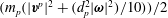 $(m_{p}(|\boldsymbol{v}^{p}|^{2}+(d_{p}^{2}|{\bf\omega}|^{2})/10))/2$
. For this reason the particular angular velocity profiles were multiplied by
$(m_{p}(|\boldsymbol{v}^{p}|^{2}+(d_{p}^{2}|{\bf\omega}|^{2})/10))/2$
. For this reason the particular angular velocity profiles were multiplied by
 $(1/10)^{1/2}d_{p}/u_{cl,0}$
to allow comparison with the particle translative velocity fluctuations shown in figure 3. The angular kinetic energy appears to be roughly 10 % of the kinetic energy in the translative velocity fluctuations.
$(1/10)^{1/2}d_{p}/u_{cl,0}$
to allow comparison with the particle translative velocity fluctuations shown in figure 3. The angular kinetic energy appears to be roughly 10 % of the kinetic energy in the translative velocity fluctuations.
3.2. The feedback force and the streamwise mean momentum equation
The attenuation of the gas-phase turbulence observed in the simulations must be caused by the feedback force, the term
 $\boldsymbol{f}$
in the equations that govern the continuous phase. To investigate this term in more detail, it is decomposed into three parts,
$\boldsymbol{f}$
in the equations that govern the continuous phase. To investigate this term in more detail, it is decomposed into three parts,
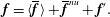 $$\begin{eqnarray}\boldsymbol{f}=\langle \overline{\boldsymbol{f}}\rangle +\overline{\boldsymbol{f}}^{nu}+\boldsymbol{f}^{\prime }.\end{eqnarray}$$
The three parts are the uniform part of the mean feedback force, the non-uniform part of the mean feedback force,
 $$\begin{eqnarray}\overline{\boldsymbol{f}}^{nu}=\overline{\boldsymbol{f}}-\langle \overline{\boldsymbol{f}}\rangle ,\end{eqnarray}$$
and the fluctuating part of the feedback force,
 $\boldsymbol{f}^{\prime }$
. The normal and spanwise components of the first two parts are negligible. The decomposition of the streamwise component of the feedback force is shown in the second column of table 3 (the uniform part of the mean force), in figure 5(a) (the non-uniform part of the mean) and in figure 5(b) (the root-mean-square profile of the fluctuation).
$\boldsymbol{f}^{\prime }$
. The normal and spanwise components of the first two parts are negligible. The decomposition of the streamwise component of the feedback force is shown in the second column of table 3 (the uniform part of the mean force), in figure 5(a) (the non-uniform part of the mean) and in figure 5(b) (the root-mean-square profile of the fluctuation).

Figure 5. Non-uniform part (a) and RMS (b) of the particle drag force in the streamwise component of the gas momentum equation,
 $\overline{f}_{1}^{nu}$
and
$\overline{f}_{1}^{nu}$
and
 $\text{RMS}(f_{1})$
, normalized with
$\text{RMS}(f_{1})$
, normalized with
 ${\it\rho}u_{{\it\tau},0}^{2}/H$
. Laden simulations A1 (solid, no markers), A2 (solid, circles) and A3 (solid, triangles). In (a) an estimate based on experimental results (KFE1994) is also shown, as described in the text.
${\it\rho}u_{{\it\tau},0}^{2}/H$
. Laden simulations A1 (solid, no markers), A2 (solid, circles) and A3 (solid, triangles). In (a) an estimate based on experimental results (KFE1994) is also shown, as described in the text.
Table 3. Domain-averaged streamwise forces (terms in the streamwise momentum equations), normalized with
 ${\it\rho}{u_{{\it\tau},0}}^{2}/H$
. The forces on the gas are listed in columns two to five. The forces on the particles are listed in columns six to eight. The quantity
${\it\rho}{u_{{\it\tau},0}}^{2}/H$
. The forces on the gas are listed in columns two to five. The forces on the particles are listed in columns six to eight. The quantity
 $\tilde{F}_{1}$
denotes
$\tilde{F}_{1}$
denotes
 $F_{1}^{p}$
summed over all particles and averaged over time. Unladen case (A0) and the three laden cases (A1 with smooth wall, A2 with rough wall, A3 with rougher wall).
$F_{1}^{p}$
summed over all particles and averaged over time. Unladen case (A0) and the three laden cases (A1 with smooth wall, A2 with rough wall, A3 with rougher wall).

Table 3 shows an overview of all terms in the domain-averaged streamwise momentum equations. The sum of the terms is zero in each case, for both the gas and particle momentum equations. The force exerted by the wall on the gas strongly increases with wall roughness. As a result the mean particle velocity profile becomes lower, and the particles exert a negative domain-averaged feedback force on the gas in the rough cases. Therefore, the streamwise pressure gradient
 ${\it\rho}\overline{a}$
needs to increase to maintain the constant gas bulk velocity in the rough cases. The effect of a larger forcing term
${\it\rho}\overline{a}$
needs to increase to maintain the constant gas bulk velocity in the rough cases. The effect of a larger forcing term
 $\overline{a}$
in single-phase flow is a larger friction velocity
$\overline{a}$
in single-phase flow is a larger friction velocity
 $u_{{\it\tau}}$
and also a larger bulk velocity
$u_{{\it\tau}}$
and also a larger bulk velocity
 $u_{b}$
and a larger mean centreline velocity
$u_{b}$
and a larger mean centreline velocity
 $u_{cl}$
or, in other words, a larger Reynolds number of the flow.
$u_{cl}$
or, in other words, a larger Reynolds number of the flow.
By definition, the uniform part of the mean feedback force does not depend on time and space, therefore it affects the flow in a similar way to
 $\overline{a}$
; in fact
$\overline{a}$
; in fact
 $g+\overline{a}+\langle \,\overline{f}_{1}\rangle$
could be lumped into a single term. The magnitude of that single term sets
$g+\overline{a}+\langle \,\overline{f}_{1}\rangle$
could be lumped into a single term. The magnitude of that single term sets
 $u_{{\it\tau}}$
and thereby the Reynolds number
$u_{{\it\tau}}$
and thereby the Reynolds number
 $Re_{{\it\tau}}$
of the flow. Thus, the effect of the mean feedback force is a change of the Reynolds number if the mean streamwise pressure gradient (
$Re_{{\it\tau}}$
of the flow. Thus, the effect of the mean feedback force is a change of the Reynolds number if the mean streamwise pressure gradient (
 ${\it\rho}\overline{a}$
) is not changed. As discussed in § 2.6,
${\it\rho}\overline{a}$
) is not changed. As discussed in § 2.6,
 $a$
is modified to maintain a constant volume flow and to have the same bulk velocity in each case. In this way the mean feedback force is not able to change the bulk Reynolds number, while the variation of
$a$
is modified to maintain a constant volume flow and to have the same bulk velocity in each case. In this way the mean feedback force is not able to change the bulk Reynolds number, while the variation of
 $u_{{\it\tau}}$
(and
$u_{{\it\tau}}$
(and
 $Re_{{\it\tau}}$
) among the different cases remains small (table 2). Comparison of the values of
$Re_{{\it\tau}}$
) among the different cases remains small (table 2). Comparison of the values of
 $\overline{a}$
in table 3 with the unladen value indicates that if we had fixed the pressure gradient, the (bulk) Reynolds number would have increased in the smooth laden case but decreased in the rough laden cases.
$\overline{a}$
in table 3 with the unladen value indicates that if we had fixed the pressure gradient, the (bulk) Reynolds number would have increased in the smooth laden case but decreased in the rough laden cases.
The non-uniform part of the feedback force, shown in figure 5(a), appears to be a monotonically decreasing function in the channel half
 $(0,H)$
for simulations A1–A3. The slope of the profile is steep in the near-wall region and zero at the centre. Thus, the non-uniformity is much stronger near the wall than in the centre region. The non-uniformity of the feedback force is apparent in each laden simulation and increases with increasing wall roughness. Provided that the particle volume fraction is uniform, the non-uniformity of the profile is directly related to the uniformity of the mean relative velocity profile,
$(0,H)$
for simulations A1–A3. The slope of the profile is steep in the near-wall region and zero at the centre. Thus, the non-uniformity is much stronger near the wall than in the centre region. The non-uniformity of the feedback force is apparent in each laden simulation and increases with increasing wall roughness. Provided that the particle volume fraction is uniform, the non-uniformity of the profile is directly related to the uniformity of the mean relative velocity profile,
 $\overline{v}_{1}-\overline{u}_{1}$
. As explained in the introduction, the mean particle velocity tends to be flatter than the mean gas velocity, such that the mean relative velocity tends to be non-uniform. It is remarked that the definition of
$\overline{v}_{1}-\overline{u}_{1}$
. As explained in the introduction, the mean particle velocity tends to be flatter than the mean gas velocity, such that the mean relative velocity tends to be non-uniform. It is remarked that the definition of
 $\overline{f}_{1}^{nu}$
implies that the volume average or the integral over
$\overline{f}_{1}^{nu}$
implies that the volume average or the integral over
 $x_{2}$
of
$x_{2}$
of
 $\overline{f}_{1}^{nu}$
is zero. This means that even for a profile
$\overline{f}_{1}^{nu}$
is zero. This means that even for a profile
 $\overline{f}_{1}$
that is non-uniform in the near-wall region only, the non-uniform part
$\overline{f}_{1}$
that is non-uniform in the near-wall region only, the non-uniform part
 $\overline{f}_{1}^{nu}$
can be non-zero in the centre region. The effect of the non-uniformity on the turbulence is not only local. Instead of the slope (derivative) of
$\overline{f}_{1}^{nu}$
can be non-zero in the centre region. The effect of the non-uniformity on the turbulence is not only local. Instead of the slope (derivative) of
 $\overline{f}_{1}^{nu}$
, it is the primitive of
$\overline{f}_{1}^{nu}$
, it is the primitive of
 $\overline{f}_{1}^{nu}$
that will appear to be tied to the Reynolds shear stress. As a global measure of the non-uniformity of the feedback force, we introduce the parameter
$\overline{f}_{1}^{nu}$
that will appear to be tied to the Reynolds shear stress. As a global measure of the non-uniformity of the feedback force, we introduce the parameter
 ${\it\beta}$
,
${\it\beta}$
,
 $$\begin{eqnarray}{\it\beta}=\frac{1}{u_{{\it\tau},0}^{2}}\int _{0}^{H}|\overline{f}_{1}^{nu}|\,\text{d}x_{2},\end{eqnarray}$$
which is in fact the normalized
 $L_{1}$
-norm of
$L_{1}$
-norm of
 $\overline{f}_{1}^{nu}$
. For simulations A1, A2 and A3, we find
$\overline{f}_{1}^{nu}$
. For simulations A1, A2 and A3, we find
 ${\it\beta}=0.43$
,
${\it\beta}=0.43$
,
 ${\it\beta}=0.73$
and
${\it\beta}=0.73$
and
 ${\it\beta}=0.87$
respectively.
${\it\beta}=0.87$
respectively.
Very flat mean particle velocity profiles have been observed in experiments in rough channels (Benson et al.
Reference Benson, Tanaka and Eaton2005). Kulick et al. (Reference Kulick, Fessler and Eaton1994) also reported that the mean particle velocity profile was flatter than the mean gas velocity profile, in particular in the near-wall region (see figure 1
b). It is appropriate to consider figure 1(b) again, since according to the experimental data for
 ${\it\phi}=0.4$
the slope of the mean particle velocity profile is not smaller than the slope of the unladen mean gas velocity profile for
${\it\phi}=0.4$
the slope of the mean particle velocity profile is not smaller than the slope of the unladen mean gas velocity profile for
 $0.7H<x_{2}<H$
. To show that nonetheless the experiments in KFE1994 do support the notion of a non-uniform part of the mean feedback force, we provide an estimate of
$0.7H<x_{2}<H$
. To show that nonetheless the experiments in KFE1994 do support the notion of a non-uniform part of the mean feedback force, we provide an estimate of
 $\overline{f}_{1}^{nu}$
based on experimental data. We define
$\overline{f}_{1}^{nu}$
based on experimental data. We define
 $$\begin{eqnarray}\overline{f}_{exp}=\frac{{\it\phi}}{{\it\tau}_{p}}\langle 1+0.15(|\overline{v}_{1}-\overline{u}_{1}|d_{p}/{\it\nu})^{0.687}\rangle (\overline{v}_{1}-\overline{u}_{1}),\end{eqnarray}$$
and substitute
 ${\it\phi}=0.8$
and
${\it\phi}=0.8$
and
 ${\it\tau}_{p}=0.131~\text{s}$
. Since for the mean particle velocity profile at
${\it\tau}_{p}=0.131~\text{s}$
. Since for the mean particle velocity profile at
 ${\it\phi}=0.8$
no experimental data are available, we approximate
${\it\phi}=0.8$
no experimental data are available, we approximate
 $\overline{v}_{1}$
by the data for
$\overline{v}_{1}$
by the data for
 ${\it\phi}=0.4$
and
${\it\phi}=0.4$
and
 ${\it\phi}=0.2$
. The two approximated
${\it\phi}=0.2$
. The two approximated
 $\overline{v}_{1}$
profiles are linearly interpolated from the experimental data. Between the wall and the measurement point nearest to the wall, the profile is horizontally extrapolated from the measurement point. This is also reasonable for the
$\overline{v}_{1}$
profiles are linearly interpolated from the experimental data. Between the wall and the measurement point nearest to the wall, the profile is horizontally extrapolated from the measurement point. This is also reasonable for the
 ${\it\phi}=0.4$
data, since the
${\it\phi}=0.4$
data, since the
 ${\it\phi}=0.2$
data show that the mean particle velocity profile is flat in the near-wall region, except for a cusp very close to the wall. For
${\it\phi}=0.2$
data show that the mean particle velocity profile is flat in the near-wall region, except for a cusp very close to the wall. For
 $\overline{v}_{1}$
taken from the
$\overline{v}_{1}$
taken from the
 ${\it\phi}=0.4$
experiment,
${\it\phi}=0.4$
experiment,
 $\overline{f}_{exp}-\langle \overline{f}_{exp}\rangle$
is shown in figure 5(a) (the domain-averaged factor in (3.4) is then 1.69). The shape of the profile is more or less similar to the shapes of
$\overline{f}_{exp}-\langle \overline{f}_{exp}\rangle$
is shown in figure 5(a) (the domain-averaged factor in (3.4) is then 1.69). The shape of the profile is more or less similar to the shapes of
 $\overline{f}_{1}^{nu}$
obtained from simulations A1–A3, although it is not monotonically decreasing on the entire channel half. The corresponding global non-uniformity parameter
$\overline{f}_{1}^{nu}$
obtained from simulations A1–A3, although it is not monotonically decreasing on the entire channel half. The corresponding global non-uniformity parameter
 ${\it\beta}$
is equal to 0.59, in between those of simulations A1 and A2. Alternatively, if
${\it\beta}$
is equal to 0.59, in between those of simulations A1 and A2. Alternatively, if
 $\overline{v}_{1}$
is taken from the
$\overline{v}_{1}$
is taken from the
 ${\it\phi}=0.2$
experiment, we find
${\it\phi}=0.2$
experiment, we find
 ${\it\beta}=0.47$
. Since the profile of the non-uniform part of the feedback force obtained with the latter estimate is very similar to the profile of simulation A1, we do not show the curve in figure 5(a), to keep the figure clearer. It is concluded that the existence of a non-uniform part of the mean feedback force is supported by experimental data.
${\it\beta}=0.47$
. Since the profile of the non-uniform part of the feedback force obtained with the latter estimate is very similar to the profile of simulation A1, we do not show the curve in figure 5(a), to keep the figure clearer. It is concluded that the existence of a non-uniform part of the mean feedback force is supported by experimental data.
Since the Reynolds shear stress is strongly modified by particles (figure 2
d), the balance of the mean streamwise momentum of the gas should also be modified. Owen (Reference Owen1969) noted the importance of the mean streamwise momentum equation, since in the context of the reduction of the gas turbulence in wall-bounded particle-laden flows he wrote in a footnote ‘in a statistically steady flow, an increasing proportion of the shear stress developed in the gas phase is transferred to the particles, in the form of a momentum flux, as the wall is approached’. In the following we consider the mean streamwise momentum equation of the gas in detail. For lower
 $Re_{{\it\tau}}$
this has been done before by Mito & Hanratty (Reference Mito and Hanratty2006) in PP-DNS of channel flow (
$Re_{{\it\tau}}$
this has been done before by Mito & Hanratty (Reference Mito and Hanratty2006) in PP-DNS of channel flow (
 $Re_{{\it\tau}}=150$
) and by Vreman (Reference Vreman2007) in PP-DNS of pipe flow (
$Re_{{\it\tau}}=150$
) and by Vreman (Reference Vreman2007) in PP-DNS of pipe flow (
 $Re_{{\it\tau}}=140$
). The derivation below shows similarities with the derivations in these papers.
$Re_{{\it\tau}}=140$
). The derivation below shows similarities with the derivations in these papers.
The streamwise component of the mean momentum equation of the gas phase can be written as
 $$\begin{eqnarray}\frac{\text{d}R_{12}}{\text{d}x_{2}}={\it\nu}\frac{\text{d}^{2}\overline{u}_{1}}{\text{d}x_{2}^{2}}+\overline{f}_{1}+g+\overline{a}.\end{eqnarray}$$
The domain-averaged mean momentum equation of the gas phase is then derived as
 $$\begin{eqnarray}-\!u_{{\it\tau}}^{2}/H+\langle \overline{f}_{1}\rangle +g+\overline{a}=0.\end{eqnarray}$$
If this equation is subtracted from (3.5), we obtain the following equation for the Reynolds shear stress:
 $$\begin{eqnarray}\frac{\text{d}R_{12}}{\text{d}x_{2}}=\frac{u_{{\it\tau}}^{2}}{H}+{\it\nu}\frac{\text{d}^{2}\overline{u}_{1}}{\text{d}x_{2}^{2}}+\overline{f}_{1}^{nu}.\end{eqnarray}$$
This is an interesting equation, as it shows the dependence of the Reynolds shear stress on the non-uniform part of the mean feedback force
 $\overline{f}_{1}^{nu}$
. This term is zero for a uniform mean feedback force, and then
$\overline{f}_{1}^{nu}$
. This term is zero for a uniform mean feedback force, and then
 $R_{12}-{\it\nu}\,\text{d}\overline{u}_{1}/\text{d}x_{1}$
is a straight line with slope
$R_{12}-{\it\nu}\,\text{d}\overline{u}_{1}/\text{d}x_{1}$
is a straight line with slope
 $u_{{\it\tau}}^{2}/H$
, like in the unladen flow. After non-dimensionalization with
$u_{{\it\tau}}^{2}/H$
, like in the unladen flow. After non-dimensionalization with
 ${\it\rho}u_{{\it\tau}}^{2}/H$
, (3.7) has the form
${\it\rho}u_{{\it\tau}}^{2}/H$
, (3.7) has the form
 $$\begin{eqnarray}\frac{H}{u_{{\it\tau}}^{2}}\frac{\text{d}R_{12}}{\text{d}x_{2}}=1+\frac{{\it\nu}H}{u_{{\it\tau}}^{2}}\frac{\text{d}^{2}\overline{u}_{1}}{\text{d}x_{2}^{2}}+\frac{H}{u_{{\it\tau}}^{2}}\overline{f}_{1}^{nu}.\end{eqnarray}$$
All terms in (3.7) have been computed for cases A1–A3: the first term on the right-hand side is shown in table 3 (after multiplication by the density), the last term on the right-hand side is shown in figure 5(a) and the left-hand side and second term on the right-hand side are shown in figure 6. The mean viscous term appears to be hardly influenced by particles and is negligible at the centre (figure 6
b); the normalized centre value is roughly
 $-0.02$
. Provided that the mean viscous term at the centre remains negligible, the slope of the Reynolds shear stress normalized with
$-0.02$
. Provided that the mean viscous term at the centre remains negligible, the slope of the Reynolds shear stress normalized with
 $u_{{\it\tau}}^{2}/H$
must decrease at the centre of the channel due to the negativity of the non-uniform part of the mean feedback force at the centre. In the present cases the effect of the particles on
$u_{{\it\tau}}^{2}/H$
must decrease at the centre of the channel due to the negativity of the non-uniform part of the mean feedback force at the centre. In the present cases the effect of the particles on
 $u_{{\it\tau}}^{2}$
is not very large; in particular, in case A2 the effect is small, approximately 1 %.
$u_{{\it\tau}}^{2}$
is not very large; in particular, in case A2 the effect is small, approximately 1 %.

Figure 6. Differentiated Reynolds shear stress (a) and the mean of the viscous term in the streamwise component of the gas momentum equation (b), normalized with
 ${\it\rho}u_{{\it\tau},0}^{2}/H$
. Laden simulations A1 (solid, no markers), A2 (solid, circles) and A3 (solid, triangles).
${\it\rho}u_{{\it\tau},0}^{2}/H$
. Laden simulations A1 (solid, no markers), A2 (solid, circles) and A3 (solid, triangles).
The integration of (3.8) between position
 $x_{2}$
and
$x_{2}$
and
 $H$
yields
$H$
yields
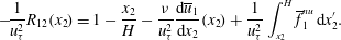 $$\begin{eqnarray}-\!\frac{1}{u_{{\it\tau}}^{2}}R_{12}(x_{2})=1-\frac{x_{2}}{H}-\frac{{\it\nu}}{u_{{\it\tau}}^{2}}\frac{\text{d}\overline{u}_{1}}{\text{d}x_{2}}(x_{2})+\frac{1}{u_{{\it\tau}}^{2}}\int _{x_{2}}^{H}\overline{f}_{1}^{nu}\,\text{d}x_{2}^{\prime }.\end{eqnarray}$$
In the derivation the properties
 $R_{12}=0$
and
$R_{12}=0$
and
 $\text{d}\overline{u}_{1}/\text{d}x_{2}=0$
at
$\text{d}\overline{u}_{1}/\text{d}x_{2}=0$
at
 $x_{2}^{\prime }=H$
have been used. Since
$x_{2}^{\prime }=H$
have been used. Since
 $\overline{f}_{1}^{nu}$
is a monotonically decreasing function of between 0 and
$\overline{f}_{1}^{nu}$
is a monotonically decreasing function of between 0 and
 $H$
and its integral between 0 and
$H$
and its integral between 0 and
 $H$
is by definition zero, we have
$H$
is by definition zero, we have
 $$\begin{eqnarray}\int _{x_{2}}^{H}\overline{f}_{1}^{nu}(x_{2}^{\prime })\,\text{d}x_{2}^{\prime }<0,\quad \text{if }0<x_{2}<H.\end{eqnarray}$$
Thus, in the case where the mean velocity profile does not change and the non-uniform part of the mean feedback force is monotonically decreasing in the interval
 $(0,H)$
, the effect of particles is a reduction of minus the Reynolds shear stress (
$(0,H)$
, the effect of particles is a reduction of minus the Reynolds shear stress (
 $-R_{12}$
) in the interval
$-R_{12}$
) in the interval
 $(0,H)$
. As long as the reduction of
$(0,H)$
. As long as the reduction of
 $-R_{12}$
is such that
$-R_{12}$
is such that
 $-R_{12}$
remains positive in the interval
$-R_{12}$
remains positive in the interval
 $(0,H)$
, this reduction is a reduction of the absolute Reynolds shear stress and thus an attenuation of an important statistical quantity of the gas turbulence. Conversely, if the Reynolds shear stress is attenuated but the mean gas velocity profile remains the same, then (3.9) shows that the mean feedback force must be non-uniform. If we define the attenuation of the Reynolds shear stress by
$(0,H)$
, this reduction is a reduction of the absolute Reynolds shear stress and thus an attenuation of an important statistical quantity of the gas turbulence. Conversely, if the Reynolds shear stress is attenuated but the mean gas velocity profile remains the same, then (3.9) shows that the mean feedback force must be non-uniform. If we define the attenuation of the Reynolds shear stress by
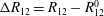 ${\rm\Delta}R_{12}=R_{12}-R_{12}^{0}$
(
${\rm\Delta}R_{12}=R_{12}-R_{12}^{0}$
(
 $R_{12}^{0}$
is the unladen profile), then the assumption of unchanged mean velocity profile implies
$R_{12}^{0}$
is the unladen profile), then the assumption of unchanged mean velocity profile implies
 $$\begin{eqnarray}-\!{\rm\Delta}R_{12}=\int _{x_{2}}^{H}\overline{f}_{1}^{nu}\,\text{d}x_{2}^{\prime },\end{eqnarray}$$
which is a direct relation between the attenuation of the Reynolds shear stress and the non-uniform part of the mean feedback force. The mean gas velocity profiles in KFE1994 are not modified by particles for mass loading ratios up to
 ${\it\phi}=0.4$
. Equation (3.11) shows that in cases where the mean gas velocity remains the same, a relatively large attenuation of
${\it\phi}=0.4$
. Equation (3.11) shows that in cases where the mean gas velocity remains the same, a relatively large attenuation of
 $R_{12}$
is equivalent to a relatively large non-uniform part of the mean feedback force. Since the turbulence attenuation of streamwise and wall-normal gas velocity fluctuations was very strong in the KFE1994 experiments, the attenuation of the Reynolds shear stress was probably also strong (the Cauchy–Schwarz inequality implies
$R_{12}$
is equivalent to a relatively large non-uniform part of the mean feedback force. Since the turbulence attenuation of streamwise and wall-normal gas velocity fluctuations was very strong in the KFE1994 experiments, the attenuation of the Reynolds shear stress was probably also strong (the Cauchy–Schwarz inequality implies
 $|R_{12}|\leqslant \text{RMS}(u_{1})\text{RMS}(u_{2})$
). It seems therefore that also the non-uniform part of the mean feedback force in these experiments must have been quite large, despite the fact that the measured mean particle velocity profile was not yet as flat as in simulations and experiments with (fully) rough walls.
$|R_{12}|\leqslant \text{RMS}(u_{1})\text{RMS}(u_{2})$
). It seems therefore that also the non-uniform part of the mean feedback force in these experiments must have been quite large, despite the fact that the measured mean particle velocity profile was not yet as flat as in simulations and experiments with (fully) rough walls.
Although the derivation above shows that the Reynolds shear stress and the non-uniform part of the mean feedback force are related, it does not prove that this non-uniformity causes the turbulence attenuation or part of the turbulence attenuation. The combination of turbulence attenuation and an unchanged mean velocity profile could also produce the non-uniformity of the drag force. Intuitively this may not be very likely, but at least there is another cause of turbulence attenuation that should be investigated, which is the fluctuating drag force. Figure 5 shows that the magnitude of the fluctuation of the drag force
 $\boldsymbol{f}^{\prime }$
is larger than the magnitude of the non-uniform part of the drag force. To investigate the role of the fluctuating drag force, we proceed with an investigation of the turbulence kinetic energy budget.
$\boldsymbol{f}^{\prime }$
is larger than the magnitude of the non-uniform part of the drag force. To investigate the role of the fluctuating drag force, we proceed with an investigation of the turbulence kinetic energy budget.
3.3. The feedback force and the turbulence kinetic energy budget
Unlike the mean feedback force, the fluctuating feedback force occurs in the turbulence kinetic energy equation of the gas phase. The corresponding term has in general a dissipative effect. It has hitherto been regarded as the mechanism by which the particle-induced turbulence attenuation should be explained.
The turbulence kinetic energy of the gas phase is defined by
 $K=(\overline{\boldsymbol{u}^{\prime }\boldsymbol{\cdot }\boldsymbol{u}^{\prime }})/2=(R_{11}+R_{22}+R_{33})/2$
. The budget or balance equation of
$K=(\overline{\boldsymbol{u}^{\prime }\boldsymbol{\cdot }\boldsymbol{u}^{\prime }})/2=(R_{11}+R_{22}+R_{33})/2$
. The budget or balance equation of
 $K$
is given by
$K$
is given by
 $$\begin{eqnarray}P_{K}+D_{K}+{\it\epsilon}_{K}+S_{K}+A_{K}=0,\end{eqnarray}$$
where
 $$\begin{eqnarray}\displaystyle & \displaystyle P_{K}=-R_{12}\frac{\text{d}\overline{u}_{1}}{\text{d}x_{2}}, & \displaystyle\end{eqnarray}$$
 $$\begin{eqnarray}\displaystyle & \displaystyle D_{K}=\frac{\text{d}}{\text{d}x_{2}}\left(-\frac{1}{2}\overline{(\boldsymbol{u}^{\prime }\boldsymbol{\cdot }\boldsymbol{u}^{\prime })u_{2}^{\prime }}-\frac{1}{{\it\rho}}\overline{P^{\prime }u_{2}^{\prime }}+{\it\nu}\frac{\text{d}K}{\text{d}x_{2}}\right), & \displaystyle\end{eqnarray}$$
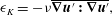 $$\begin{eqnarray}\displaystyle & {\it\epsilon}_{K}=-{\it\nu}\overline{\boldsymbol{{\rm\nabla}}\boldsymbol{u}^{\prime }\boldsymbol{ : }\boldsymbol{{\rm\nabla}}\boldsymbol{u}^{\prime }}, & \displaystyle\end{eqnarray}$$
 $$\begin{eqnarray}\displaystyle & S_{K}=\overline{\boldsymbol{u}^{\prime }\boldsymbol{\cdot }\boldsymbol{f}^{\prime }}, & \displaystyle\end{eqnarray}$$
 $$\begin{eqnarray}\displaystyle & A_{K}=\overline{a^{\prime }u_{1}^{\prime }}. & \displaystyle\end{eqnarray}$$
 $P_{K}$
is the turbulence production,
$P_{K}$
is the turbulence production,
 $D_{K}$
is the sum of turbulent diffusion, pressure diffusion and viscous diffusion,
$D_{K}$
is the sum of turbulent diffusion, pressure diffusion and viscous diffusion,
 ${\it\epsilon}_{K}$
is minus the turbulence dissipation and
${\it\epsilon}_{K}$
is minus the turbulence dissipation and
 $S_{K}$
is a particle-induced energy source term (often negative). The term
$S_{K}$
is a particle-induced energy source term (often negative). The term
 $A_{K}$
is the correlation between the streamwise velocity fluctuation and the fluctuation of the domain-averaged pressure gradient. Since
$A_{K}$
is the correlation between the streamwise velocity fluctuation and the fluctuation of the domain-averaged pressure gradient. Since
 $A_{K}$
is expected to be small, the term is usually omitted, but its negligibility should be verified if
$A_{K}$
is expected to be small, the term is usually omitted, but its negligibility should be verified if
 $a$
is a function of time.
$a$
is a function of time.

Figure 7. Turbulence kinetic energy budget in the near-wall region: turbulence production
 $P_{K}$
(a), total diffusion
$P_{K}$
(a), total diffusion
 $D_{K}$
(b), turbulence dissipation
$D_{K}$
(b), turbulence dissipation
 ${\it\epsilon}_{K}$
(c) and particle-induced source term
${\it\epsilon}_{K}$
(c) and particle-induced source term
 $S_{K}$
(d), normalized with
$S_{K}$
(d), normalized with
 $u_{{\it\tau},0}^{3}/H$
. Unladen DNS A0 (dashed) and the laden simulations A1 (solid, no markers), A2 (solid, circles) and A3 (solid, triangles).
$u_{{\it\tau},0}^{3}/H$
. Unladen DNS A0 (dashed) and the laden simulations A1 (solid, no markers), A2 (solid, circles) and A3 (solid, triangles).
The budget of turbulence kinetic energy is shown in figure 7 (for the near-wall region) and in figure 8 (for the core region). The term
 $A_{K}$
is not shown, since its absolute value normalized with
$A_{K}$
is not shown, since its absolute value normalized with
 $u_{{\it\tau},0}^{3}/H$
was less than 0.003, negligible indeed. It is observed that all other terms in the budget are strongly affected by the particles. In particular, the turbulence production is reduced across the entire channel, the turbulence dissipation is reduced, while the reduction of
$u_{{\it\tau},0}^{3}/H$
was less than 0.003, negligible indeed. It is observed that all other terms in the budget are strongly affected by the particles. In particular, the turbulence production is reduced across the entire channel, the turbulence dissipation is reduced, while the reduction of
 $D_{K}$
in the centre region of the channel shows that also turbulence transport from the wall to the centre is strongly inhibited by the particle motion. The term
$D_{K}$
in the centre region of the channel shows that also turbulence transport from the wall to the centre is strongly inhibited by the particle motion. The term
 $S_{K}$
is interesting in particular; it has since long been recognized that this term plays an important role in turbulence attenuation (Elghobashi & Truesdell Reference Elghobashi and Truesdell1993). It is the correlation between the fluctuating feedback force and the fluctuating gas velocity. The correlation tends to be negative if the standard drag law is used and the particle fluctuation and fluid fluctuation are decorrelated. If the second condition is not fulfilled, the term may be positive. In regions with weak gas turbulence but strong particle velocity fluctuation, the instantaneous oscillations of gas regions produced by particles that cross the region may be larger than the turbulence generated by (nonlinear) channel flow instabilities. Gas fluctuations created by particle fluctuations are probably positively correlated, which tends to make
$S_{K}$
is interesting in particular; it has since long been recognized that this term plays an important role in turbulence attenuation (Elghobashi & Truesdell Reference Elghobashi and Truesdell1993). It is the correlation between the fluctuating feedback force and the fluctuating gas velocity. The correlation tends to be negative if the standard drag law is used and the particle fluctuation and fluid fluctuation are decorrelated. If the second condition is not fulfilled, the term may be positive. In regions with weak gas turbulence but strong particle velocity fluctuation, the instantaneous oscillations of gas regions produced by particles that cross the region may be larger than the turbulence generated by (nonlinear) channel flow instabilities. Gas fluctuations created by particle fluctuations are probably positively correlated, which tends to make
 $S_{K}$
positive. Very close to the wall
$S_{K}$
positive. Very close to the wall
 $S_{K}$
is positive for A1–A3, while at the channel centre
$S_{K}$
is positive for A1–A3, while at the channel centre
 $S_{K}$
is positive in cases A2 and A3. In cases A2 and A3, the turbulence attenuation is strong, and the particle velocity fluctuations are large. Thus, the particles produce some turbulence kinetic energy, which is immediately dissipated by viscosity. The latter contributes to the viscous dissipation, which possibly explains why the centreline dissipation of case A3 is hardly reduced compared with the (small) unladen dissipation.
$S_{K}$
is positive in cases A2 and A3. In cases A2 and A3, the turbulence attenuation is strong, and the particle velocity fluctuations are large. Thus, the particles produce some turbulence kinetic energy, which is immediately dissipated by viscosity. The latter contributes to the viscous dissipation, which possibly explains why the centreline dissipation of case A3 is hardly reduced compared with the (small) unladen dissipation.

Figure 8. Turbulence kinetic energy budget in the core region: turbulence production
 $P_{K}$
(a), total diffusion
$P_{K}$
(a), total diffusion
 $D_{K}$
(b), turbulence dissipation
$D_{K}$
(b), turbulence dissipation
 ${\it\epsilon}_{K}$
(c) and particle-induced source term
${\it\epsilon}_{K}$
(c) and particle-induced source term
 $S_{K}$
(d), normalized with
$S_{K}$
(d), normalized with
 $u_{{\it\tau},0}^{3}/H$
. Unladen DNS A0 (dashed) and the laden simulations A1 (solid, no markers), A2 (solid, circles) and A3 (solid, triangles).
$u_{{\it\tau},0}^{3}/H$
. Unladen DNS A0 (dashed) and the laden simulations A1 (solid, no markers), A2 (solid, circles) and A3 (solid, triangles).
Perhaps the most surprising feature of the energy budget equation is that strong turbulence attenuation is possible, while the quantity
 $S_{K}$
remains relatively small. In case A3, the domain average of
$S_{K}$
remains relatively small. In case A3, the domain average of
 $S_{K}$
is approximately zero, such that the term has no net dissipative effect, although the turbulence attenuation is strong. As discussed in § 3.1, Hwang & Eaton (Reference Hwang and Eaton2006) found that a point-particle model of
$S_{K}$
is approximately zero, such that the term has no net dissipative effect, although the turbulence attenuation is strong. As discussed in § 3.1, Hwang & Eaton (Reference Hwang and Eaton2006) found that a point-particle model of
 $S_{K}$
underpredicts the dissipation by particles in isotropic turbulence if
$S_{K}$
underpredicts the dissipation by particles in isotropic turbulence if
 $d_{p}\gtrapprox {\it\eta}$
, see also Balachandar & Eaton (Reference Balachandar and Eaton2010). Nevertheless, the observation that a simulation of the Navier–Stokes equations shows strong turbulence attenuation in a case where the feedback term has no net dissipative effect remains surprising.
$d_{p}\gtrapprox {\it\eta}$
, see also Balachandar & Eaton (Reference Balachandar and Eaton2010). Nevertheless, the observation that a simulation of the Navier–Stokes equations shows strong turbulence attenuation in a case where the feedback term has no net dissipative effect remains surprising.
We finish this section with a brief discussion of the influence of the Reynolds number on turbulence attenuation. In the present PP-DNS of gas–solid channel flow with smooth walls at mass loading ratio 0.8 and
 $Re_{{\it\tau}}=642$
, the turbulence is significantly reduced but still relevant. However, in a PP-DNS of gas–solid pipe flow with smooth walls at a similar mass loading ratio, 0.77, but lower Reynolds number,
$Re_{{\it\tau}}=642$
, the turbulence is significantly reduced but still relevant. However, in a PP-DNS of gas–solid pipe flow with smooth walls at a similar mass loading ratio, 0.77, but lower Reynolds number,
 $Re_{{\it\tau}}=140$
, the gas-phase turbulence production, the Reynolds shear stress and also the radial diagonal component of the Reynolds stress tensor were negligibly small, less than 10 % of the unladen values (Vreman Reference Vreman2007). Although pipe flow and channel flow are not equivalent, this comparison seems to suggest that turbulence attenuation becomes less pronounced with increasing Reynolds number.
$Re_{{\it\tau}}=140$
, the gas-phase turbulence production, the Reynolds shear stress and also the radial diagonal component of the Reynolds stress tensor were negligibly small, less than 10 % of the unladen values (Vreman Reference Vreman2007). Although pipe flow and channel flow are not equivalent, this comparison seems to suggest that turbulence attenuation becomes less pronounced with increasing Reynolds number.
4. The effect of a non-uniform mean feedback force
4.1. Direct numerical simulation of turbulent channel flow with non-uniform forcing
Turbulence attenuation in particle-laden channel flows is often attributed (solely) to the fluctuating feedback force, since that is the only part of the feedback force that appears in the particle-induced source term
 $S_{K}$
in the turbulence kinetic energy equation. However, (4.7) shows that an important statistical quantity of the turbulence, the Reynolds shear stress, is related to the primitive of the non-uniform part of the mean feedback force, in particular if the mean gas velocity profile is not much affected. This leads to the hypothesis that a non-uniform part of the mean feedback force acts as one of the causes of turbulence attenuation in particle-laden channel flow. So far, this is only an hypothesis, because the possibility that the non-uniform part of the mean feedback force is not a cause but just a consequence of turbulence attenuation has not been ruled out yet.
$S_{K}$
in the turbulence kinetic energy equation. However, (4.7) shows that an important statistical quantity of the turbulence, the Reynolds shear stress, is related to the primitive of the non-uniform part of the mean feedback force, in particular if the mean gas velocity profile is not much affected. This leads to the hypothesis that a non-uniform part of the mean feedback force acts as one of the causes of turbulence attenuation in particle-laden channel flow. So far, this is only an hypothesis, because the possibility that the non-uniform part of the mean feedback force is not a cause but just a consequence of turbulence attenuation has not been ruled out yet.
To demonstrate that a non-uniform feedback force is able to attenuate the turbulence by itself, three additional direct numerical simulations are performed, B1–B3, in which the effect of the mean feedback force is isolated. Unlike A1–A3, these simulations do not use the point-particle model, at least not explicitly. Simulation B1 is a DNS of the Navier–Stokes equations with forcing
 $\boldsymbol{f}=f_{1}(x_{2})\boldsymbol{e}_{\mathbf{1}}$
. Thus, in these cases
$\boldsymbol{f}=f_{1}(x_{2})\boldsymbol{e}_{\mathbf{1}}$
. Thus, in these cases
 $f_{2}=f_{3}=0$
and
$f_{2}=f_{3}=0$
and
 $f_{1}$
is a function of
$f_{1}$
is a function of
 $x_{2}$
only. The function
$x_{2}$
only. The function
 $f_{1}$
in simulation B1 is precisely the mean feedback force of simulation A1. Similarly, simulations B2 and B3 use the mean feedback forces of simulations A2 and A3 respectively. The fluctuating feedback force is not used in simulations B1–B3. Like in simulations A1–A3, the domain average of the streamwise pressure gradient (
$f_{1}$
in simulation B1 is precisely the mean feedback force of simulation A1. Similarly, simulations B2 and B3 use the mean feedback forces of simulations A2 and A3 respectively. The fluctuating feedback force is not used in simulations B1–B3. Like in simulations A1–A3, the domain average of the streamwise pressure gradient (
 ${\it\rho}a$
) is adapted to fix the bulk velocity in B1–B3 to
${\it\rho}a$
) is adapted to fix the bulk velocity in B1–B3 to
 $9.212~\text{m}~\text{s}^{-1}$
. Thus, the turbulence modification in B1 (B2, B3) compared with case A0 can only be caused by the profile of the non-uniform part of the mean feedback force A1 (A2, A3). That profile is shown in figure 5(a).
$9.212~\text{m}~\text{s}^{-1}$
. Thus, the turbulence modification in B1 (B2, B3) compared with case A0 can only be caused by the profile of the non-uniform part of the mean feedback force A1 (A2, A3). That profile is shown in figure 5(a).
The results of simulations B1–B3 are shown in figure 9. It appears that the turbulence is also significantly attenuated in these cases, although the attenuation is not as strong as in cases A1–A3. For example, in case B1 the centreline value of the streamwise (wall-normal) fluctuation is reduced by 33 % (26 %); in case A1 it was reduced by 34 % (44 %). The spanwise velocity fluctuation, not shown for these cases, is attenuated in a similar way to the wall-normal velocity fluctuation. The attenuation observed in cases B1–B3 cannot be caused by
 $S_{K}$
, the particle-induced source term in the turbulence kinetic energy equation, since this term is zero in these cases (
$S_{K}$
, the particle-induced source term in the turbulence kinetic energy equation, since this term is zero in these cases (
 $\boldsymbol{f}^{\prime }=0$
). This means that the attenuation in B1–B3 must be caused by the mean streamwise feedback force. Wall roughness makes the mean particle force more non-uniform (figure 5
a), and simulations B1–3 show that stronger non-uniformity leads to more turbulence attenuation.
$\boldsymbol{f}^{\prime }=0$
). This means that the attenuation in B1–B3 must be caused by the mean streamwise feedback force. Wall roughness makes the mean particle force more non-uniform (figure 5
a), and simulations B1–3 show that stronger non-uniformity leads to more turbulence attenuation.

Figure 9. Mean streamwise velocity
 $\overline{u}_{1}$
(a),
$\overline{u}_{1}$
(a),
 $\text{RMS}(u_{1})$
(b),
$\text{RMS}(u_{1})$
(b),
 $\text{RMS}(u_{2})$
(c) and Reynolds shear stress
$\text{RMS}(u_{2})$
(c) and Reynolds shear stress
 $R_{12}$
(d), normalized with the unladen centreline velocity
$R_{12}$
(d), normalized with the unladen centreline velocity
 $u_{cl,0}$
. Results from four direct numerical simulations: A0 (dashed), B1 (solid, no markers), B2 (solid, circles) and B3 (solid, triangles). The forcing in B1–B3 is
$u_{cl,0}$
. Results from four direct numerical simulations: A0 (dashed), B1 (solid, no markers), B2 (solid, circles) and B3 (solid, triangles). The forcing in B1–B3 is
 $\overline{f}_{1}\boldsymbol{e}_{\mathbf{1}}$
with the mean force
$\overline{f}_{1}\boldsymbol{e}_{\mathbf{1}}$
with the mean force
 $\overline{f}_{1}$
taken from A1, A2 and A3 respectively.
$\overline{f}_{1}$
taken from A1, A2 and A3 respectively.
While the difference between case B1 (B2, B3) and the unladen case A0 gives an estimate of the contribution of the mean feedback force to the turbulence modification in case A1 (A2, A3), the difference between case A1 (A2, A3) and case B1 (B2, B3) gives an estimate of the contribution of the fluctuation of the feedback force to the turbulence modification in case A1 (A2, A3). Both contributions turn out to be significant.
Compared with the modification of the velocity fluctuations and the Reynolds shear stress, the modification of the mean velocity profile in cases B1–B3 is small, in particular in case B1; in cases B2 and B3 the effects on the linear profile are somewhat larger than in cases A2 and A3. The friction velocity
 $u_{{\it\tau}}$
is equal to
$u_{{\it\tau}}$
is equal to
 $0.490~\text{m}~\text{s}^{-1}$
,
$0.490~\text{m}~\text{s}^{-1}$
,
 $0.496~\text{m}~\text{s}^{-1}$
,
$0.496~\text{m}~\text{s}^{-1}$
,
 $0.501~\text{m}~\text{s}^{-1}$
and
$0.501~\text{m}~\text{s}^{-1}$
and
 $0.504~\text{m}~\text{s}^{-1}$
in cases A0, B1, B2 and B3 respectively. The bulk velocity is by definition the same in each case. The centreline velocity
$0.504~\text{m}~\text{s}^{-1}$
in cases A0, B1, B2 and B3 respectively. The bulk velocity is by definition the same in each case. The centreline velocity
 $u_{cl}$
is equal to
$u_{cl}$
is equal to
 $10.42~\text{m}~\text{s}^{-1}$
,
$10.42~\text{m}~\text{s}^{-1}$
,
 $10.40~\text{m}~\text{s}^{-1}$
,
$10.40~\text{m}~\text{s}^{-1}$
,
 $10.08~\text{m}~\text{s}^{-1}$
and
$10.08~\text{m}~\text{s}^{-1}$
and
 $9.97~\text{m}~\text{s}^{-1}$
in cases A0, B1, B2 and B3 respectively. Thus, with increasing non-uniformity of the forcing,
$9.97~\text{m}~\text{s}^{-1}$
in cases A0, B1, B2 and B3 respectively. Thus, with increasing non-uniformity of the forcing,
 $u_{{\it\tau}}$
increases slightly and
$u_{{\it\tau}}$
increases slightly and
 $u_{cl}$
decreases slightly; in other words the mean profile becomes less rounded. How can this be reconciled with case A2, in which both
$u_{cl}$
decreases slightly; in other words the mean profile becomes less rounded. How can this be reconciled with case A2, in which both
 $u_{{\it\tau}}$
and
$u_{{\it\tau}}$
and
 $u_{cl}$
were almost identical to
$u_{cl}$
were almost identical to
 $u_{{\it\tau},0}$
and
$u_{{\it\tau},0}$
and
 $u_{cl,0}$
? The smaller change of the mean gas velocity profile in case A2 compared with B2 can only be explained by an interplay of the non-uniform part of the mean feedback force and the fluctuating feedback force. Both parts attenuate the turbulence. However, the non-uniform mean part tends to make the mean profile less rounded, while the fluctuating part tends to make the mean profile more rounded. These two effects on the mean gas velocity profile cancel to certain extent; this is most clearly visible in case A2.
$u_{cl,0}$
? The smaller change of the mean gas velocity profile in case A2 compared with B2 can only be explained by an interplay of the non-uniform part of the mean feedback force and the fluctuating feedback force. Both parts attenuate the turbulence. However, the non-uniform mean part tends to make the mean profile less rounded, while the fluctuating part tends to make the mean profile more rounded. These two effects on the mean gas velocity profile cancel to certain extent; this is most clearly visible in case A2.
4.2. Linear stability analysis
As another illustration of the response of the Navier–Stokes equations to a feedback force with a non-uniform mean part, a linear stability analysis is performed. We consider the linear instability of a laminar velocity profile to two-dimensional perturbations, as described by the Orr–Sommerfeld equations (Criminale, Jackson & Joslin Reference Criminale, Jackson and Joslin2003). In linear stability theory the flow is decomposed into a base profile
 $U(x_{2})$
and a velocity perturbation fluctuation proportional to the Fourier mode
$U(x_{2})$
and a velocity perturbation fluctuation proportional to the Fourier mode
 $\exp (\text{i}({\it\alpha}_{1}x_{1}-{\it\gamma}t))$
, where
$\exp (\text{i}({\it\alpha}_{1}x_{1}-{\it\gamma}t))$
, where
 $\text{i}=(-1)^{1/2}$
,
$\text{i}=(-1)^{1/2}$
,
 ${\it\alpha}_{1}$
is a prescribed streamwise spatial wavenumber and the frequency
${\it\alpha}_{1}$
is a prescribed streamwise spatial wavenumber and the frequency
 ${\it\gamma}$
is the complex eigenvalue.
${\it\gamma}$
is the complex eigenvalue.
For simplicity of the analysis we consider a linear version of the feedback force,
 $\boldsymbol{f}=c(\boldsymbol{v}-\boldsymbol{u})$
, with
$\boldsymbol{f}=c(\boldsymbol{v}-\boldsymbol{u})$
, with
 $c=({\it\phi}/{\it\tau}_{p})(1+0.15R^{0.687})$
, where the constant
$c=({\it\phi}/{\it\tau}_{p})(1+0.15R^{0.687})$
, where the constant
 $R$
is a representative particle Reynolds number which does not depend on time and space. As a further simplification, we assume that the particles move with a uniform velocity,
$R$
is a representative particle Reynolds number which does not depend on time and space. As a further simplification, we assume that the particles move with a uniform velocity,
 $\boldsymbol{v}=V\boldsymbol{e}_{\mathbf{1}}$
, where
$\boldsymbol{v}=V\boldsymbol{e}_{\mathbf{1}}$
, where
 $V$
is a constant. Since
$V$
is a constant. Since
 $c$
is uniform, the value of the uniform particle velocity
$c$
is uniform, the value of the uniform particle velocity
 $V$
is irrelevant for the flow dynamics, since
$V$
is irrelevant for the flow dynamics, since
 $cV$
,
$cV$
,
 $g$
and
$g$
and
 $a$
can be lumped into a single parameter
$a$
can be lumped into a single parameter
 $b=g+a+cV$
.
$b=g+a+cV$
.
The unperturbed momentum equation of the linearized problem becomes
 $$\begin{eqnarray}{\it\nu}\frac{\text{d}^{2}U}{\text{d}{x_{2}}^{2}}-cU+b=0,\end{eqnarray}$$
and
 $U(0)=U(2H)=0$
. The analytical solution of this equation is
$U(0)=U(2H)=0$
. The analytical solution of this equation is
 $$\begin{eqnarray}U(x_{2})=U_{0}\frac{\text{cosh}({\it\lambda}H)-\text{cosh}({\it\lambda}x_{2}-{\it\lambda}H)}{\text{cosh}({\it\lambda}H)-1},\end{eqnarray}$$
where
 $U_{0}$
denotes the centreline velocity and
$U_{0}$
denotes the centreline velocity and
 ${\it\lambda}^{2}=c/{\it\nu}$
. The constants
${\it\lambda}^{2}=c/{\it\nu}$
. The constants
 $b$
and
$b$
and
 $U_{0}$
are related by
$U_{0}$
are related by
 $$\begin{eqnarray}b=\frac{cU_{0}\text{cosh}({\it\lambda}H)}{\text{cosh}({\it\lambda}H)-1}.\end{eqnarray}$$
Three examples of base profiles
 $U(x_{2})$
are shown in figure 10(a). For
$U(x_{2})$
are shown in figure 10(a). For
 ${\it\lambda}\rightarrow 0$
, the profile converges to the standard parabolic profile
${\it\lambda}\rightarrow 0$
, the profile converges to the standard parabolic profile
 $U_{0}x_{2}(2H-x_{2})/H^{2}$
, while for
$U_{0}x_{2}(2H-x_{2})/H^{2}$
, while for
 ${\it\lambda}\rightarrow \infty$
, the profile converges to
${\it\lambda}\rightarrow \infty$
, the profile converges to
 $U_{0}$
for
$U_{0}$
for
 $0<x_{2}<2H$
.
$0<x_{2}<2H$
.
The Orr–Sommerfeld equation for the eigenfunction of the normal velocity component, denoted by
 $\hat{u} _{2}(x_{2})$
, reads
$\hat{u} _{2}(x_{2})$
, reads
 $$\begin{eqnarray}\left(U-\frac{{\it\gamma}}{{\it\alpha}_{1}}\right)(\hat{u} _{2}^{\prime \prime }-{\it\alpha}_{1}^{2}\hat{u} _{2})-U^{\prime \prime }\hat{u} _{2}=\frac{1}{\text{i}{\it\alpha}_{1}}[{\it\nu}({\hat{u} _{2}}^{\prime \prime \prime \prime \prime }-2{\it\alpha}_{1}^{2}{\hat{u} _{2}}^{\prime \prime }+{\it\alpha}_{1}^{4}\hat{u} _{2})-c({\hat{u} _{2}}^{\prime \prime }-{\it\alpha}_{1}\hat{u} _{2})],\end{eqnarray}$$
where the prime denotes differentiation with respect to
 $x_{2}$
. The non-conventional term proportional to
$x_{2}$
. The non-conventional term proportional to
 $c$
represents the fluctuating feedback force. The equation above can be derived from the evolution equation of the Laplacian of the normal component of the velocity perturbation, following the procedure described in Criminale et al. (Reference Criminale, Jackson and Joslin2003).
$c$
represents the fluctuating feedback force. The equation above can be derived from the evolution equation of the Laplacian of the normal component of the velocity perturbation, following the procedure described in Criminale et al. (Reference Criminale, Jackson and Joslin2003).
The linear growth rate Im(
 ${\it\gamma}$
), the imaginary part of
${\it\gamma}$
), the imaginary part of
 ${\it\gamma}$
, is shown in figure 10(b) for several cases, all for
${\it\gamma}$
, is shown in figure 10(b) for several cases, all for
 $Re=U_{0}H/{\it\nu}=14\,000$
, roughly the same as the Reynolds number based on the mean centreline velocity of the unladen DNS. It appears that a very modest flattening of the base flow (
$Re=U_{0}H/{\it\nu}=14\,000$
, roughly the same as the Reynolds number based on the mean centreline velocity of the unladen DNS. It appears that a very modest flattening of the base flow (
 ${\it\lambda}=1$
) leads to a strong reduction of the most unstable growth rate. Comparison with a case with the mean feedback force, but without the fluctuating feedback force (
${\it\lambda}=1$
) leads to a strong reduction of the most unstable growth rate. Comparison with a case with the mean feedback force, but without the fluctuating feedback force (
 ${\it\lambda}=1$
in (4.2) and
${\it\lambda}=1$
in (4.2) and
 $c=0$
in (4.4)), shows that the linear stabilization is primarily caused by the mean feedback component which slightly changes the parabolic profile. The critical value for
$c=0$
in (4.4)), shows that the linear stabilization is primarily caused by the mean feedback component which slightly changes the parabolic profile. The critical value for
 ${\it\lambda}$
is approximately 1.3; for
${\it\lambda}$
is approximately 1.3; for
 ${\it\lambda}>1.3$
the system is linearly stable for all
${\it\lambda}>1.3$
the system is linearly stable for all
 ${\it\alpha}_{1}$
.
${\it\alpha}_{1}$
.

Figure 10. (a) Base velocity profile in the linear stability theory (4.2) for
 ${\it\lambda}\rightarrow 0$
(red dashed),
${\it\lambda}\rightarrow 0$
(red dashed),
 ${\it\lambda}=1$
(blue solid) and
${\it\lambda}=1$
(blue solid) and
 ${\it\lambda}=10$
(black squares). (b) Linear growth rate (normalized by
${\it\lambda}=10$
(black squares). (b) Linear growth rate (normalized by
 $U_{0}/H$
) as a function of the streamwise wavenumber
$U_{0}/H$
) as a function of the streamwise wavenumber
 ${\it\alpha}$
(normalized by
${\it\alpha}$
(normalized by
 $H^{-1}$
) for
$H^{-1}$
) for
 ${\it\lambda}\rightarrow 0$
(red dashed), for
${\it\lambda}\rightarrow 0$
(red dashed), for
 ${\it\lambda}=1$
and
${\it\lambda}=1$
and
 $c={\it\lambda}^{2}{\it\nu}$
(blue solid), and for
$c={\it\lambda}^{2}{\it\nu}$
(blue solid), and for
 ${\it\lambda}=1$
and
${\it\lambda}=1$
and
 $c=0$
(black dash–dotted).
$c=0$
(black dash–dotted).
4.3. The equation of the velocity fluctuation
Since the mean feedback force does not occur in the turbulence kinetic energy equation or in any of the equations of the Reynolds stresses, the question may arise of how a non-uniform mean feedback force can contribute to significant turbulence attenuation. It is tempting to assume that the mean feedback force can only modify the turbulence via a modification of the mean gas velocity profile, which does explicitly appear in the Reynolds stress equations. However, the mean gas velocity profile is not necessarily significantly modified, consider for example case A2. According to this argument, the mean feedback force cannot play an important role in the turbulence attenuation, at least not in case A2. In the following we will indicate where this intuitively logical argument fails.
The presumption in the argument is that the Reynolds stress equations and the mean flow are all that is required to describe the turbulence. This is not correct. Even if the mean velocity profile is prescribed, the Reynolds stress equations do not form a closed set. The argument would be valid if it were possible to close the unclosed terms (for example turbulence transport, pressure strain and turbulence dissipation) by algebraic models in terms of the Reynolds stresses and the mean velocity profile. However, an accurate closure of this type is unknown and may not exist. Of course, additional transport equations can be derived for the unclosed expressions, but then these additional equations will suffer from similar closure problems.
These closure problems are avoided if we consider the system of equations for the mean and instantaneous fluctuation of the gas velocity. For simplicity, we assume that the forcing term
 $\boldsymbol{f}$
is known as input as a vector field that varies in time and space. The following system is then a closed system for the mean and fluctuation of the gas velocity:
$\boldsymbol{f}$
is known as input as a vector field that varies in time and space. The following system is then a closed system for the mean and fluctuation of the gas velocity:
 $$\begin{eqnarray}\displaystyle & \displaystyle \frac{\partial \boldsymbol{u}^{\prime }}{\partial t}=-\boldsymbol{u}^{\prime }\boldsymbol{\cdot }\boldsymbol{{\rm\nabla}}\boldsymbol{u}^{\prime }-\frac{1}{{\it\rho}}\boldsymbol{{\rm\nabla}}P^{\prime }+{\it\nu}{\rm\nabla}^{2}\boldsymbol{u}^{\prime }-\overline{u}_{1}\frac{\partial \boldsymbol{u}^{\prime }}{\partial x_{1}}+\left(\frac{\text{d}\overline{u_{1}^{\prime }u_{2}^{\prime }}}{\text{d}x_{2}}-u_{2}^{\prime }\frac{\text{d}\overline{u}_{1}}{\text{d}x_{2}}+a^{\prime }\right)\boldsymbol{e}_{\mathbf{1}}+\boldsymbol{f}^{\prime }, & \displaystyle\end{eqnarray}$$
 $$\begin{eqnarray}\displaystyle & \boldsymbol{{\rm\nabla}}\boldsymbol{\cdot }\boldsymbol{u}^{\prime }=0, & \displaystyle\end{eqnarray}$$
 $$\begin{eqnarray}\displaystyle & \displaystyle \frac{\text{d}\overline{u_{1}^{\prime }u_{2}^{\prime }}}{\text{d}x_{2}}=\frac{u_{{\it\tau}}^{2}}{H}+{\it\nu}\frac{\text{d}^{2}\overline{u}_{1}}{\text{d}x_{2}^{2}}+\overline{f}_{1}^{nu}, & \displaystyle\end{eqnarray}$$
 $$\begin{eqnarray}\displaystyle & \langle \overline{u}_{1}\rangle =u_{b,0}, & \displaystyle\end{eqnarray}$$
 $$\begin{eqnarray}\displaystyle & \displaystyle a^{\prime }=-{\it\nu}\left\langle \frac{\partial ^{2}u_{1}^{\prime }}{\partial x_{2}^{2}}\right\rangle -\langle f_{1}^{\prime }\rangle , & \displaystyle\end{eqnarray}$$
 $u_{b,0}$
is the prescribed gas bulk velocity and the expression for
$u_{b,0}$
is the prescribed gas bulk velocity and the expression for
 $a^{\prime }$
follows from the requirement that the domain-averaged streamwise velocity remains constant,
$a^{\prime }$
follows from the requirement that the domain-averaged streamwise velocity remains constant,
 $\text{d}\langle u_{1}\rangle /\text{d}t=0$
. This is a complete system of integro-differential equations for the unknowns
$\text{d}\langle u_{1}\rangle /\text{d}t=0$
. This is a complete system of integro-differential equations for the unknowns
 $\boldsymbol{u}^{\prime }$
,
$\boldsymbol{u}^{\prime }$
,
 $P^{\prime }$
,
$P^{\prime }$
,
 $\overline{u}_{1}$
and
$\overline{u}_{1}$
and
 $a^{\prime }$
, for given
$a^{\prime }$
, for given
 $\boldsymbol{f}$
,
$\boldsymbol{f}$
,
 $u_{b,0}$
, initial condition for
$u_{b,0}$
, initial condition for
 $\boldsymbol{u}^{\prime }$
and no-slip boundary conditions for
$\boldsymbol{u}^{\prime }$
and no-slip boundary conditions for
 $\boldsymbol{u}^{\prime }$
and
$\boldsymbol{u}^{\prime }$
and
 $\overline{u}_{1}$
. The unknown
$\overline{u}_{1}$
. The unknown
 $a^{\prime }$
can easily be eliminated by substitution of the last equation into (4.5).
$a^{\prime }$
can easily be eliminated by substitution of the last equation into (4.5).
In the above system only (4.5) contains a time derivative; only this equation is an evolution equation, the other equations are additional constraints. One constraint is the incompressibility constraint, another one is (4.7). In other words, the field
 $\boldsymbol{u}^{\prime }$
can only evolve such that the statistical average of
$\boldsymbol{u}^{\prime }$
can only evolve such that the statistical average of
 $u_{1}^{\prime }u_{2}^{\prime }$
satisfies a constraint in which the non-uniform part of the mean feedback force explicitly appears. Thus, although the mean feedback force does not explicitly appear in (4.5), this does not mean that
$u_{1}^{\prime }u_{2}^{\prime }$
satisfies a constraint in which the non-uniform part of the mean feedback force explicitly appears. Thus, although the mean feedback force does not explicitly appear in (4.5), this does not mean that
 $\boldsymbol{u}^{\prime }$
would not depend on it. To clarify this further, we substitute (4.7) into (4.5), assume
$\boldsymbol{u}^{\prime }$
would not depend on it. To clarify this further, we substitute (4.7) into (4.5), assume
 $a^{\prime }=0$
(then
$a^{\prime }=0$
(then
 $\text{d}\langle u_{1}\rangle /\text{d}t$
is not necessarily zero), skip (4.8) and prescribe
$\text{d}\langle u_{1}\rangle /\text{d}t$
is not necessarily zero), skip (4.8) and prescribe
 $u_{{\it\tau}}=u_{{\it\tau},0}$
. We obtain
$u_{{\it\tau}}=u_{{\it\tau},0}$
. We obtain
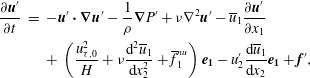 $$\begin{eqnarray}\displaystyle \frac{\partial \boldsymbol{u}^{\prime }}{\partial t} & = & \displaystyle -\boldsymbol{u}^{\prime }\boldsymbol{\cdot }\boldsymbol{{\rm\nabla}}\boldsymbol{u}^{\prime }-\frac{1}{{\it\rho}}\boldsymbol{{\rm\nabla}}P^{\prime }+{\it\nu}{\rm\nabla}^{2}\boldsymbol{u}^{\prime }-\overline{u}_{1}\frac{\partial \boldsymbol{u}^{\prime }}{\partial x_{1}}\nonumber\\ \displaystyle & & \displaystyle +\,\left(\frac{u_{{\it\tau},0}^{2}}{H}+{\it\nu}\frac{\text{d}^{2}\overline{u}_{1}}{\text{d}x_{2}^{2}}+\overline{f}_{1}^{nu}\right)\boldsymbol{e}_{\mathbf{1}}-u_{2}^{\prime }\frac{\text{d}\overline{u}_{1}}{\text{d}x_{2}}\boldsymbol{e}_{\mathbf{1}}+\boldsymbol{f}^{\prime },\end{eqnarray}$$
 $$\begin{eqnarray}\displaystyle & \boldsymbol{{\rm\nabla}}\boldsymbol{\cdot }\boldsymbol{u}^{\prime }=0, & \displaystyle\end{eqnarray}$$
 $$\begin{eqnarray}\displaystyle & \displaystyle \frac{\text{d}\overline{u_{1}^{\prime }u_{2}^{\prime }}}{\text{d}x_{2}}=\frac{u_{{\it\tau},0}^{2}}{H}+{\it\nu}\frac{\text{d}^{2}\overline{u}_{1}}{\text{d}x_{2}^{2}}+\overline{f}_{1}^{nu}, & \displaystyle\end{eqnarray}$$
 $\boldsymbol{u}^{\prime }$
,
$\boldsymbol{u}^{\prime }$
,
 $P^{\prime }$
and
$P^{\prime }$
and
 $\overline{u}_{1}$
, for given
$\overline{u}_{1}$
, for given
 $\overline{f}_{1}^{nu}$
,
$\overline{f}_{1}^{nu}$
,
 $\boldsymbol{f}^{\prime }$
,
$\boldsymbol{f}^{\prime }$
,
 $u_{{\it\tau},0}$
, initial condition for
$u_{{\it\tau},0}$
, initial condition for
 $\boldsymbol{u}^{\prime }$
and no-slip boundary conditions for
$\boldsymbol{u}^{\prime }$
and no-slip boundary conditions for
 $\boldsymbol{u}^{\prime }$
and
$\boldsymbol{u}^{\prime }$
and
 $\overline{u}_{1}$
. In this formulation the fluctuating velocity explicitly depends on the non-uniform part of the mean feedback force. If we contract (4.10) with
$\overline{u}_{1}$
. In this formulation the fluctuating velocity explicitly depends on the non-uniform part of the mean feedback force. If we contract (4.10) with
 $\boldsymbol{u}^{\prime }$
, the product
$\boldsymbol{u}^{\prime }$
, the product
 $u_{1}^{\prime }\overline{f}_{1}^{nu}$
appears. The mean of this product is zero, and that is why it does not appear in the statistical turbulence kinetic energy equation. Although
$u_{1}^{\prime }\overline{f}_{1}^{nu}$
appears. The mean of this product is zero, and that is why it does not appear in the statistical turbulence kinetic energy equation. Although
 $\overline{f}_{1}^{nu}$
has no mean dissipative effect, it can modify the dynamics of
$\overline{f}_{1}^{nu}$
has no mean dissipative effect, it can modify the dynamics of
 $\boldsymbol{u}^{\prime }$
, and the consequence may be that statistical correlations that do appear in the turbulence kinetic energy equation (production, transport and dissipation) are reduced. The appearance of
$\boldsymbol{u}^{\prime }$
, and the consequence may be that statistical correlations that do appear in the turbulence kinetic energy equation (production, transport and dissipation) are reduced. The appearance of
 $\overline{f}_{1}^{nu}$
in the equation of
$\overline{f}_{1}^{nu}$
in the equation of
 $\boldsymbol{u}^{\prime }$
is a nonlinear effect. In linear stability theory all terms that are quadratic in
$\boldsymbol{u}^{\prime }$
is a nonlinear effect. In linear stability theory all terms that are quadratic in
 $\boldsymbol{u}^{\prime }$
vanish; in particular, the left-hand side of (4.12) is then replaced by zero, such that the sum of the three terms between brackets in (4.10) also vanishes.
$\boldsymbol{u}^{\prime }$
vanish; in particular, the left-hand side of (4.12) is then replaced by zero, such that the sum of the three terms between brackets in (4.10) also vanishes.
5. Conclusions
Point-particle direct numerical simulations of downward particle-laden vertical channel flows were performed. In order to investigate the effect of wall roughness on particle-induced turbulence attenuation, both smooth and rough walls were applied in the simulations. Inter-particle collisions were included. A new element in the computational method was that wall roughness was taken into account with a deterministic instead of a stochastic model. The wall roughness was represented by packed layers of spherical particles attached to the wall. The diameter of these fixed wall particles was smaller than the viscous wall unit. The mass loading ratio of the particle-laden channel was 0.8, and the Reynolds number (of the unladen case) was equal to
 $Re_{{\it\tau}}=642$
. Previous simulations of turbulence attenuation in the literature were either performed at lower Reynolds number or the PP-LES method was used.
$Re_{{\it\tau}}=642$
. Previous simulations of turbulence attenuation in the literature were either performed at lower Reynolds number or the PP-LES method was used.
As an answer to the first research question formulated in the introduction, we found that wall roughness enhances the turbulence attenuation in vertical particle-laden channel flow, at least when the size of the wall roughness is sufficiently small. This was not obvious, since the same conclusion was only known from experiments of horizontal channel flow (Kussin & Sommerfeld Reference Kussin and Sommerfeld2002), while the available experimental results in vertical channel flow did not show attenuation of the turbulence (Benson et al. Reference Benson, Tanaka and Eaton2005). This can be explained, as it now seems, by the fact that the roughness size in the latter experiments was, albeit not very large in terms of wall units, much higher than in the experiments of Kussin & Sommerfeld (Reference Kussin and Sommerfeld2002) and in the simulations in the present paper.
The effect of wall roughness is that the mean particle velocity profile, which is also in smooth channel flow flatter than the mean gas velocity profile, is flattened further. As a consequence, the non-uniformity of the mean feedback force is increased. Non-uniformity of the mean feedback force is one of the causes of turbulence attenuation in particle-laden channel flow. The latter was shown by DNS of single-phase flow with non-uniform forcings. In each of these cases, the non-uniform forcing was a mean feedback force profile from a PP-DNS. Moreover, in these additional simulations significant turbulence attenuation was found, albeit not as strong as in the point-particle simulations. The attenuation increased with increased non-uniformity of the mean forcing term. It is concluded that not only the fluctuating component but also the (non-uniform) mean component of the particle force contributes to turbulence attenuation. The combined effect of both components on the mean gas velocity is relatively small, because the mean component tends to flatten and the fluctuating component tends to round the mean gas velocity profile. Furthermore, a linear stability analysis was performed, which showed that not only turbulent fluctuations, but also the linear growth rate of the perturbation superimposed on a laminar profile, is reduced by a non-uniform mean particle force.
Any PP-DNS is only a pseudo-DNS, since particle boundary layers and wakes are not resolved. This limitation and possible consequences were discussed. It would be interesting to resimulate the cases studied in this work with particle-resolved DNS. Hopefully this will be possible one day.
Acknowledgements
The author has been granted permission to use his knowledge of the efficient particle collision software developed by J. A. M. Kuipers, B. P. M. Hoomans, J. M. Link, G. A. Bokkers and N. G. Deen (Hoomans et al. Reference Hoomans, Kuipers, Briels and van Swaaij1996). The code used for the simulations in the present paper does not contain any part of this software, but the knowledge has helped the author to develop his own efficient particle collision subroutines.


 Open access