


1. INTRODUCTION
In marine and air navigation, ships and aircraft sailing or flying on fixed compass headings may travel along Rhumb Lines (RL), hence knowledge of RL calculation is important. Mercator's projection (a normal aspect cylindrical conformal projection) has the unique property that RLs on the Earth's surface are projected as straight lines on the map.
Methods of calculating the course and the distance between two points from knowledge of their latitudes and longitudes, or calculating the latitude and the longitude of the arrival point from the course and the distance from a known departure point, are called ‘sailings’. A RL appears as a straight line on a Mercator chart and as a spiral curve (Loxodrome) on a surface of an oblate spheroid. Both of these cut all the meridians at the same angle (Thomas, Reference Thomas1952; Williams, Reference Williams1998). The distance for a RL on the navigation sphere is within 0·5% of the distance on the RL on the WGS84 spheroid (Earle, Reference Earle2006) Figure 1.

Figure 1. Rhumb Line (Loxodrome) on the Earth's surface.
In geodesy or navigation, the ‘direct’ problem (computing position given azimuth and distance from a known location) and the ‘inverse’ problem (computing azimuth and distance between known positions) are fundamental operations and can be likened to the equivalent operations of plane surveying. ‘Radiations’ (computing coordinates of points given bearings and distances radiating from a point of known coordinates) and ‘joins’; (computing bearings and distances between points having known coordinates) are terms frequently used.
Solutions to the direct and inverse problem together constitute what is called the ‘complete’ solution. The terms ‘direct’ and ‘inverse’ in geodesy are usually associated with the geodesic, which is the unique curve defining the shortest path on the ellipsoid, but they can also be associated with other curves.
The direct solution for Rhumb Line Sailing (RLS) on the oblate spheroid is often treated by schemes that require iterative methods (Snyder, Reference Snyder1987; Tseng, Reference Tseng2006). Though adequate results have been achieved, the need for iterative methods has persisted without necessarily realizing higher accuracies (Bennett, Reference Bennett1996). Furthermore, interpolation for latitude in terms of longitude between end points of a RL on the spheroid has not yet been found in the literature. As a consequence of these observations, the complete solution to RLS presented here will include a method to determine latitude for any longitude along the RL. The accuracies attained can satisfy the requirement of ECDIS and GIS environments.
2. THE DIFFERENTIAL EQUATION OF THE RHUMB LINE
In rectangular coordinates, points such as P on the oblate spheroid (Figure 2) have coordinates:
where:
β is reduced or parametric latitude.
a is the semi-major axis.
b is the semi-minor axis.
There are various ways of specifying the dimensions of the spheroid other than by its major and minor radii. The flattening, f, is defined by f=1-b/a, and the eccentricity e by e 2=1-b 2/a 2. For the World Geodetic System 1984 (WGS 84), a=6378137 m and f=298·257223563.

Figure 2. Meridian on a spheroid.
A displacement of dβ in reduced latitude along the meridian is illustrated in Figure 3. The displacements of three axes can be obtained by partial differentiating P with respect to reduced latitude:
The displacement parallel to the z-axis is bcosβ and the displacement towards the z-axis is –asinβ. The geodetic and reduced latitude are related by:
The radius of altitude parallel (Figure 3) is given by:
The result of a displacement of dβ in reduced latitude and of dλ in longitude is illustrated in Figure 3.These displacements together cause a displacement acosβdλ eastward and a displacement a(1−e 2 cos2β)1/2dβ northward, respectively.

Figure 3. Triangles resulting from infinitesimal latitude and longitude changes.
By Pythagoras's theorem the displacement ds is given by:
Substituting Equation (3) into Equation (5) yields the following:
RLs are paths of constant true course. They thus satisfy the following:
This is most easily treated in geodetic latitude. Integrating Equation (7) yields:
where MP(φ′), as used here, is the distance in meridional parts.
‘Meridional parts’ are defined as the length of the arc of a meridian between the Equator and a given parallel (geodetic latitude φ′) on a Mercator chart, expressed in units of 1 minute of longitude at the Equator. Thus:
Combining Equation (6) and (7) with constant true course gives an integral for arc length along the RL.
where R m=a(1−ε 2)(1−ε 2 sin2θ)−3/2 is the radius of curvature of meridian.
3. SOLUTIONS FOR RHUMB LINE SAILING
The arc-length of a meridian is the primary element for direct and inverse solutions to RLS. The above integral, Equation (6), can be approximated by a truncated series in the square of the eccentricity upon expanding the integrand in a binomial series:
In Equation (11) and Equation (12) below, each term of the binomial series for half integer multiples is defined by:
Using trigonometric identities, the powers of the sine term may be reduced to combinations of cosine terms of the form cos(2·i·φ). Collecting terms with the same cosine arguments and integrating gives the following series:
where:
Expansion of coefficients for Equation (12) was facilitated using computer symbolic processing. These coefficients are shown below truncated at order e10 and M 10. Those up to M 8, first given by (Delambre, Reference Delambre1799) were used for confirmation of the results:
3.1. RLS Direct Solution
The direct problem computes the arrival position given azimuth and distance to be travelled from a known location. The distance S(φ 1) to departure point P 1 from the Equator is first established and added to ∆S, the distance to be travelled. Thus the overall distance from the Equator is:
Application of the Lagrange Inversion Theorem (Adams, Reference Adams1921) or Hermite Interpolation Scheme produces the inverse solution of meridian arc-length so as to determine latitude from meridional distance. It is very difficult or even impossible, to derive the necessary high order derivatives by hand. Fortunately, modern computer aided symbolic algebra found in mathematical software packages mitigates the effort required (e.g., Mathematica™, Maple™ or MATLAB™).
Figure 4 shows the construction of the problem to be solved. Two known components of the RL having an azimuth α are shown in blue and red. The objective is to determine geodetic co-ordinates φ, λ of the end point.

Figure 4. Direct problem of RLS.
Geodetic latitude as a function of distance from the Equator has been determined as just described through manipulation of Equation (10) to determine its inverse relationship. This inverse function gives geodetic latitude as in terms of the rectifying latitude μ:
where distance S(φ) is transformed into the rectifying latitude by:
and for which the coefficients of sin(2·i·φ) are:
Once the geodetic end point or arrival latitude has been determined, the arrival longitude can be established from:
The tangent of true course (tan α) becomes infinity when true course is East or West. In which case, RL distance is along a parallel at the latitude of departure. Latitude and longitude of end point are then set by:
3.2. RLS Inverse Solution
The inverse problem, as indicated in Figure 5, determines the true azimuth and the distance between two points given the departure and destination coordinates. Since the end points are known, azimuth is determined from application of Equation (8) to the end point latitudes to obtain the true course of the RL.

Figure 5. Inverse problem of RLS.
Equation (21) maps an angle λ−λ 1 (in radians) to the interval [−π π] and gives Δλ correctly as:
where ceil (x) rounds the elements of x to the smallest integer greater than or equal to x.
The RL distance between two latitudes is next calculated with Equation (12). So then:
Since the tangent of true course (tan α) becomes infinity for East or West courses, Equation (12) cannot be applied to calculate the distance. In which case, the RL distance is the arc-length of part of the parallel at the latitude of departure given by:
3.3. Interpolation of the Rhumb Line at Other Longitudes
Once a RL has been determined between two end points, it may be required to determine the latitude at one or more other longitudes between end points. Equation (8) provides the longitude in terms of latitude. The geodetic latitude of any point along the RL can be determined once the longitude and true course have been specified. Figure 6 shows a RL for which latitude φ is to be found for an arbitrary longitude λ.

Figure 6. Latitude in terms of longitude.
First, application of Equation (8) gives the meridional parts at a given longitude along RL:
Secondly, the conformal latitude δ associated with MP(φ 1) can be obtained from the following:
which is equivalent to:
or:
The inversion of Equation (27) has once again been accomplished via the Lagrange Inversion Theorem (Adams, 1927) or the Hermite Interpolation Scheme. Computer symbolic algebra was again used to determine coefficients of a series for conformal latitude. The resulting expression for geodetic latitude in terms of conformal latitude (Adams, 1927; Thomas, Reference Thomas1952; Snyder, Reference Snyder1987) is then:
Expanding to O(e8), terms for K are approximately given by.
4. NUMERICAL TEST
A ship steers from a departure point at F (40°43′N, 74°00′W) to a destination at T (55°45′S, 37°37′E) along the RL on the WGS84 Earth (Figure 7). Course and distance are initially determined from the given end points using Equations (20) and (22). Latitudes and longitudes of waypoints beyond departure point at F at distances of 1000, 2000, … nautical miles are then found after using Equations (15) and (18). Results are shown in Table 1.

Figure 7. A ship steers from F (40°43 ′N, 74°00′W) to T (55°45 ′S, 37°37′E).
Table 1. Positions differing in distance and recovered distances and courses. Applied Equations: (15), (18), (20) and (22).

For each value of latitude and longitude calculated at each waypoint, Equations (20) and (22) are applied to recover their corresponding values of course and distance as shown in Table 1 in the columns for Course* and Distance*. It can be seen that the resulting differences are negligible as shown in Table 1, Column 6 (Distance Error) and Column 8 (Course Error).
In another test for recovered longitude, the latitudes of waypoints beyond the departure point F located at 70° W, 60° W, 50°W, … , 30° E (Figure 8) are first found after using Equations (24), (27), and (28) and are shown in Table 2, column 2 (Latitude).
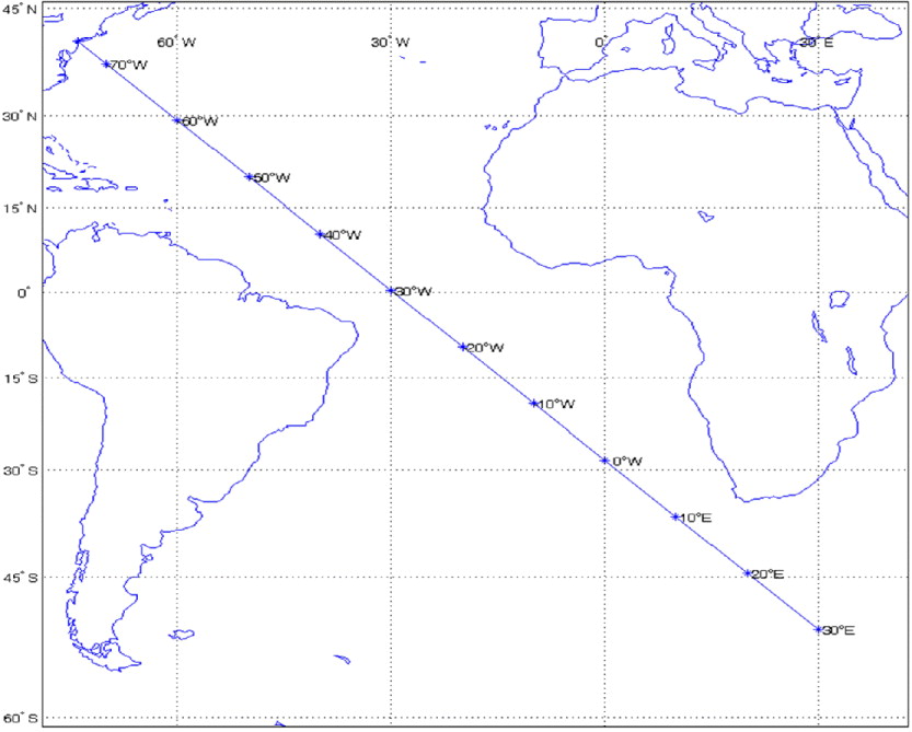
Figure 8. Sampling by Given Longitude.
Table 2. Latitude in terms of Longitude and Recovered Longitude. Applied equations: (18), (24), (27), and (28).
On applying Equation (18) using the calculated latitude shown in Table 2, column 2 (Latitude), the recovered longitude was then calculated as shown in Table 2, column 3. The resulting differences when compared with the given values of Table 2, column 1 are also negligible as shown in Table 2, column 4 (Error).
5. CONCLUSIONS
Accurate solutions to the direct and inverse problems of Rhumb Line Sailing (RLS) have been described and demonstrated. These two solutions provide useful alternatives to previous approaches in that they require no recourse to integrals or iteration methods. The solution for latitude in terms of longitude has also been described and demonstrated. This was achieved by application of an inverse expansion of conformal latitude that gives very accurate latitude in terms of longitude without iteration.
These three series along with the formula for meridional parts are seen to be simple, direct and computationally efficient. They provide positioning accuracies involving distance, position, and true course that are in the sub-metre range and which are also commensurate with the current levels of accuracy achieved by Global Navigation Satellite Systems (GNSS), while at the same time, they provide a complete solution to RLS. The algorithms provided here are easily incorporated into computer software and are well suited to vessel route planning and cartographical computation in Graphical Information System (GIS) and Electronic Chart Display and Information System (ECDIS) environments.
ACKNOWLEDGEMENTS
This work was supported in part by the National Science Council of Taiwan, Republic of China, under grant NSC 98-2410-H-019-019-, NSC 99-2410-H-019-023-, and NSC 100-2410-H-019-018-.


