2.1 Problem formulation

In the present study, the quasi-one-dimensional approximation is used to model the steady flow of a mono-component single-phase fluid through a converging–diverging nozzle. The quasi-one-dimensional governing equations for smooth, i.e. shock-free, flows are the well-known algebraic equations enforcing the conservation of mass, of total enthalpy and entropy, namely

(2.1a ) $$\begin{eqnarray}\displaystyle & \displaystyle {\it\rho}uA(x)=\text{const.}, & \displaystyle\end{eqnarray}$$

(2.1b ) $$\begin{eqnarray}\displaystyle & \displaystyle h+{\textstyle \frac{1}{2}}u^{2}=\text{const.}, & \displaystyle\end{eqnarray}$$

(2.1c ) $$\begin{eqnarray}\displaystyle & \displaystyle s=\text{const.}, & \displaystyle\end{eqnarray}$$

${\it\rho}$

$u$

$h$

$A(x)$

$x$

Discontinuous solutions including shock waves are accounted for by means of the well-known Rankine–Hugoniot jump relations. The locus of thermodynamic states that can possibly be connected by a shock wave, if drawn in the $P$ – $v$ plane, is referred to as the shock adiabat. If the pre-shock state is fixed, the shock adiabat determines the relation between the pressure and the specific volume of the post-shock state. However, the post-shock state satisfying the jump conditions for a given pre-shock state is, in general, not unique. The Rankine–Hugoniot relations must be supplemented with suitable admissibility criteria in order to rule out unphysical solutions. One sufficient condition is that shock waves arise as limits of travelling-wave profiles including viscosity and heat conduction (see Menikoff & Plohr Reference Menikoff and Plohr1989; Kluwick Reference Kluwick2001). This admissibility criterion has a direct and convenient graphical interpretation: the straight segment connecting the pre-shock and post-shock states in the $P$ – $v$ plane (commonly referred to as the Rayleigh line) must be located either completely above or completely below the shock adiabat centred on the pre-shock state. In the first case, the shock wave carries a positive pressure jump (compression shock); in the second one the shock carries a negative pressure jump (expansion or rarefaction shock). Note that shock waves admitting viscous profiles also satisfy the well-known entropy condition $s_{B}\geqslant s_{A}$ and the speed ordering relation $M_{A}\geqslant 1\geqslant M_{B}$ , where subscripts $A$ and $B$ denote pre-shock and post-shock quantities, respectively (Lax Reference Lax1957; Oleinik Reference Oleinik1959).

In order to complete the problem, a suitable thermodynamic model of the fluid must be specified. In this work, we consider fluids described by the model of van der Waals (Reference van der Waals1873) with constant isochoric heat capacity $c_{v}$ , namely

(2.2a,b ) $$\begin{eqnarray}\displaystyle P(T,v)=\frac{RT}{v-b}-\frac{a}{v^{2}},\quad c_{v}=\text{const.}, & & \displaystyle\end{eqnarray}$$

where $R$ is the gas constant, $T$ is the temperature and the constants $a$ and $b$ account for the excluded volume and for the intermolecular forces, respectively. Thanks to its simplicity, the van der Waals model with constant $c_{v}$ (also referred to as the polytropic van der Waals model) has frequently been employed in studies on negative and mixed nonlinearities (see, e.g. Cramer & Sen Reference Cramer and Sen1986; Cramer Reference Cramer and Kluwick1991; Argrow Reference Argrow1996; Brown & Argrow Reference Brown and Argrow1997; Müller & Voß Reference Müller and Voß2006). Indeed, as pointed out by many authors (see, e.g. Thompson & Lambrakis Reference Thompson and Lambrakis1973; Kluwick Reference Kluwick2001; Guardone, Vigevano & Argrow Reference Guardone, Vigevano and Argrow2004; Guardone & Argrow Reference Guardone and Argrow2005), the polytropic van der Waals model predicts the correct qualitative behaviour in the thermodynamic region of interest in this work, though it is admittedly less accurate with respect to more complex thermodynamic models (see Martin & Hou Reference Martin and Hou1955; Martin, Kapoor & De Nevers Reference Martin, Kapoor and De Nevers1959; Peng & Robinson Reference Peng and Robinson1976; Span & Wagner Reference Span and Wagner2003a ,Reference Span and Wagner b ).

Moreover, analytical equations of state, including the van der Waals model considered here, fail to predict the fluid thermodynamics in the very close proximity of the liquid–vapour critical point. The divergence of properties near the critical point is properly described in terms of scaling laws, see for example the scaling laws proposed by Levelt-Sengers (Reference Levelt-Sengers1970), Levelt-Sengers, Greer & Sengers (Reference Levelt-Sengers, Greer and Sengers1976) and Levelt-Sengers, Morrison & Chang (Reference Levelt-Sengers, Morrison and Chang1983). Non-classical gasdynamic in the critical region was studied by Emanuel (Reference Emanuel1996) and more recently by Nannan, Guardone & Colonna (Reference Nannan, Guardone and Colonna2013, Reference Nannan, Guardone and Colonna2014) and Nannan et al. (Reference Nannan, Sirianni, Mathijssen, Guardone and Colonna2016). In particular, in Nannan et al. (Reference Nannan, Guardone and Colonna2013), a comparison is made between analytical thermodynamic models and scaling laws in terms of the predicted values of ${\it\Gamma}$ and a significant departure was observed only in very close proximity to the critical point ( $|T/T_{c}-1|<0.01$ ). The thermodynamic region of interest here is sufficiently far from the critical point to rely on analytical models and the analysis of nozzle flows in very close proximity to the liquid–vapour critical point is left for future investigations.

2.2 Isentropic flow

According to the governing equations (2.1), the mass flow rate ${\dot{m}}={\it\rho}uA(x)$ and the total enthalpy $h^{t}=h+u^{2}/2$ are uniform both in shock-free and in shocked flows. The entropy $s$ , on the other hand, is piece-wise uniform with finite jumps occurring across shock waves. Therefore, most non-classical effects occurring in quasi-1D steady nozzle flows can be explained in a comprehensive manner by examining the basic properties of isentropic flows with constant total enthalpy.

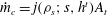
Figure 1. Variation of the Mach number (a) and of the mass flux function (b) along exemplary isentropes, as computed from the polytropic van der Waals model with $c_{v}/R=50$ . The total enthalpy is constant, $h^{t}=h(1.0182P_{c},v_{c})$ .

We start by commenting on the relation between the Mach number $M=u/c=\sqrt{2(h^{t}-h)}/c$ and the density in non-ideal compressible-fluid flows. Following Cramer & Best (Reference Cramer and Best1991), the first derivative of $M$ is recast in non-dimensional form as

(2.3) $$\begin{eqnarray}\displaystyle J={\displaystyle \frac{{\it\rho}}{M}}{\displaystyle \frac{\text{d}M}{\text{d}{\it\rho}}}=1-{\it\Gamma}-{\displaystyle \frac{1}{M^{2}}}. & & \displaystyle\end{eqnarray}$$

In flows of fluids with ${\it\Gamma}>1$ (perfect gases, for instance), the Mach number always decreases upon isentropic compression. Conversely, in fluid flows exhibiting ${\it\Gamma}<1$ , the Mach number can possibly increase with density. The variation of the Mach number along exemplary isentropic flows computed from the van der Waals model with $c_{v}/R=50$ is sketched in figure 1(a). The current fluid model specifications correspond to a BZT fluid and will be used throughout the present work. The $M$ – ${\it\rho}$ diagram shown in figure 1(a) is generated for a fixed value of the total enthalpy. Thus, each curve corresponds to a different entropy value along the same isenthalpic line $h=h^{t}$ . Isentropes in figure 1(a) intersect the liquid–vapour phase boundary along curve labelled $M^{sat}$ . A wide portion of the saturated vapour boundary of the fluid considered is retrograde (see Thompson, Carofano & Kim Reference Thompson, Carofano and Kim1986; Menikoff & Plohr Reference Menikoff and Plohr1989), meaning that isentropes cross the phase boundary from the mixed towards the pure phase, in the direction of decreasing density. However, all isentropes eventually enter the two-phase region crossing a non-retrograde saturated phase boundary. The intersection with the non-retrograde portion of the saturated vapour boundary occurs at such low density values, compared to those characterizing the thermodynamic region of interest in this work, that it is reasonable to assume that isentropes cross saturation boundaries only if $s<s_{vle}$ , where $s_{vle}$ denotes the isentrope tangent to the vapour dome. The present analysis is limited to the single-phase portions of any given isentrope. Two-phase effects, as well as critical point phenomena which affect near-to-critical isentropes, are outside the scope of this work.

The locus $J=0$ in figure 1(a) gathers all stationary points in the Mach number-density plot and its general form can be explained by analysing the evolution of ${\it\Gamma}$ along isentropes featuring ${\it\Gamma}<1$ (see, e.g. Bethe Reference Bethe1942; Zel’dovich Reference Zel’dovich1946; Thompson & Lambrakis Reference Thompson and Lambrakis1973). On these isentropes, ${\it\Gamma}-1$ has only two zeros with a local minimum in between, where ${\it\Lambda}=\left(\partial {\it\Gamma}/\partial {\it\rho}\right)_{s}$  vanishes. We differentiate (2.3) to obtain, after evaluation at $J=0$ ,

(2.4) $$\begin{eqnarray}\displaystyle \left.{\displaystyle \frac{\text{d}^{2}M}{\text{d}{\it\rho}^{2}}}\right|_{J=0}=-{\displaystyle \frac{M}{{\it\rho}}}{\it\Lambda}. & & \displaystyle\end{eqnarray}$$

Thus, with reference to figure 1(a), stationary points of the Mach number located at higher densities ( ${\it\Lambda}>0$ ) and at lower densities ( ${\it\Lambda}<0$ ) of the ${\it\Lambda}=0$ locus are local maxima and minima, respectively.

Isentropes corresponding to sufficiently large stagnation densities must cross the $J>0$ region. We restrict the discussion to those curves that remain in the single-phase region during a full expansion from stagnation conditions to vacuum. In this case, isentropes entering the $J>0$ region exhibit both a local minimum and a local maximum of the Mach number. If the latter occurs at sufficiently high Mach numbers, the flow remains supersonic upon further expansion. On the other hand, if the local maximum is only slightly supersonic, the flow becomes subsonic inside the $J>0$ region. As a result, the selected isentrope exhibits three sonic points. By decreasing the stagnation density, the two stationary points become subsonic and eventually merge in a stationary inflection point. If the stagnation density is further decreased, the Mach number ultimately becomes a monotone decreasing function of the density.

Figure 2. Phase planes for selected isentropes featuring (a) one sonic point and (b,c) three sonic points upon isentropic expansion with constant total enthalpy. Dashed segments denote sonic values of the density, ordered as ${\it\rho}_{s_{3}}<{\it\rho}_{s_{2}}<{\it\rho}_{s_{1}}$ . If one sonic point only is present, it is specified as ${\it\rho}_{s_{\text{}}}$ . (b) The lowest of the sonic densities corresponds to the global maximum of the related mass flux function. (c) The largest of the sonic densities corresponds to the global maximum of the related mass flux function.

Next, we consider the variation of the mass flux function $j={\it\rho}\sqrt{2(h^{t}-h)}$ in isentropic flows with constant total enthalpy. Firstly, $j$ varies with ${\it\rho}$ according to

(2.5) $$\begin{eqnarray}\displaystyle {\displaystyle \frac{1}{c}}{\displaystyle \frac{\text{d}j}{\text{d}{\it\rho}}}={\displaystyle \frac{M^{2}-1}{M}}. & & \displaystyle\end{eqnarray}$$

Thus, the mass flux function increases (decreases) upon supersonic (subsonic) isentropic compression and sonic points are extrema. In addition, given that

(2.6) $$\begin{eqnarray}\displaystyle {\displaystyle \frac{{\it\rho}}{c}}\left.{\displaystyle \frac{\text{d}^{2}j}{\text{d}{\it\rho}^{2}}}\right|_{M=1}=-2{\it\Gamma}, & & \displaystyle\end{eqnarray}$$

a sonic point is a local maximum, minimum or stationary inflection point of the mass flux if ${\it\Gamma}$ is positive, negative or null at that point, respectively. A similar analysis was performed by Kluwick (Reference Kluwick1993, Reference Kluwick2004), albeit in the context of small perturbations in transonic flows. Figure 1(b) illustrates exemplary mass flux functions corresponding to different entropy values chosen along the isenthalpic locus $h=h^{t}$ .

In this respect, it is instructive to analyse the phase plane related to such isentropic flows, i.e. the contour plot of the mass flow rate ${\dot{m}}=jA(x)$ in the ${\it\rho}$ – $x$ plane. In this study, all plots refer to a converging–diverging nozzle described by a fifth-order polynomial, whose coefficients are computed to set the inlet area $A_{i}=1.2$ , the throat area $A_{t}=1$ and an exit area $A_{e}=1.5$ , and by imposing that the inlet, the throat and the exit stations are stationary points of the area distribution.

Isentropes containing a single sonic point generate saddle-shaped phase planes, see figure 2(a). The relevant value

(2.7) $$\begin{eqnarray}\displaystyle {\dot{m}}_{c}=\max _{{\it\rho}}j({\it\rho};s,h^{t})\min _{x}A(x) & & \displaystyle\end{eqnarray}$$

corresponds to the saddle point and is referred to as the critical mass flow rate. In the present case ${\dot{m}}_{c}=j({\it\rho}_{s_{\text{}}};s,h^{t})A_{t}$ , where ${\it\rho}_{s_{\text{}}}$ is the (unique) sonic density. Given that we are interested in the expansion from a reservoir, we will naturally focus on subsonic inlet conditions. Curves such as $a$ in figure 2(a) display ${\dot{m}}<{\dot{m}}_{c}$ and result in strictly subsonic flows. The curve labelled $b$ in figure 2(a) corresponds to ${\dot{m}}={\dot{m}}_{c}$ . Subsonic–supersonic transition is possible, as well as completely subsonic flow with sonic throat. Along curves such as curve $c$ , which display ${\dot{m}}>{\dot{m}}_{c}$ , sonic conditions occur upstream of the throat and the flow cannot be continued beyond this point. These trajectories have no physical relevance in steady isentropic flows discharging from a still reservoir.

The flows we are mainly interested in are those associated with isentropes including three sonic points. Phase planes related to such isentropes exhibit two saddle points with a local minimum in between. Given the following ordering for the sonic values of the density,

(2.8) $$\begin{eqnarray}\displaystyle {\it\rho}_{s_{3}}<{\it\rho}_{s_{2}}<{\it\rho}_{s_{1}}, & & \displaystyle\end{eqnarray}$$

two different categories of phase plane were defined by Cramer & Fry (Reference Cramer and Fry1993), depending on which of the local maxima is the global one.

The case 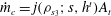${\dot{m}}_{c}=j({\it\rho}_{s_{3}};s,h^{t})A_{t}$ is depicted in figure 2(b). We follow Cramer & Fry (Reference Cramer and Fry1993) in referring to this kind of non-classical phase plane as Type-2. In figure 2(b), in addition to the possible cases presented in figure 2(a), there exist feasible paths (e.g. contour lines going from the inlet section to the outlet section) in which sonic conditions are encountered either upstream or downstream of the throat. For example, if ${\dot{m}}=j({\it\rho}_{s_{1}};s,h^{t})A_{t}$ , the curve labelled $b$ is generated which corresponds to a flow that is sonic both at the throat ( ${\it\rho}={\it\rho}_{s_{1}}$ ) and in the diverging section ( ${\it\rho}={\it\rho}_{s_{2}}$ ). However, in the latter sonic condition, the slope $\text{d}{\it\rho}/\text{d}x$ goes to infinity and the trajectory has a turning point. Therefore, the flow cannot be continued isentropically beyond this sonic point. Curves labelled $c$ ( ${\dot{m}}<{\dot{m}}_{c}$ ) and $d$ ( ${\dot{m}}={\dot{m}}_{c}$ ) also include multiple sonic points and, such as in case b, these paths cannot be accomplished in an isentropic flow.

Figure 2(c) describes the case ${\dot{m}}_{c}=j({\it\rho}_{s_{1}};s,h^{t})A_{t}$ , which is referred to as a Type-1 phase plane in accordance with the nomenclature proposed by Cramer & Fry (Reference Cramer and Fry1993). Significant trajectories with subsonic inlet are those of type $a$ ( ${\dot{m}}<{\dot{m}}_{c}$ ) and $b$ ( ${\dot{m}}={\dot{m}}_{c}$ ). The latter cannot be continued beyond sonic point ${\it\rho}_{s_{2}}$ , which occurs downstream of the throat. By using an approximate isentropic model, i.e. neglecting the entropy rise across shock waves, Cramer & Fry (Reference Cramer and Fry1993) depicted expected flow configurations including several non-classical shock waves. The phase plane analysis predicts the formation of non-classical flow fields along paths including three sonic points, see also Kluwick (Reference Kluwick1993). Trajectories such as $b$ , $c$ and $d$ in figure 2(b) or $b$ in figure 2(c) are indeed realizable and represent branches of shocked flows, yet the insertion of sonic shocks is required where sonic conditions occur upstream or downstream of the throat. In such cases, flows with arbitrarily large exit Mach numbers cannot be realized isentropically, as is the case in classical nozzle flows of ideal gases.

2.3 Isentropic patterns

The general properties of a quasi-1D isentropic flow, such as the number of sonic points and the layout of the corresponding phase plane, delineate a so-called isentropic pattern. We propose a classification of quasi-1D isentropic flows into five different isentropic patterns, as detailed in table 1. In the following, symbol $\mathscr{S}$ will be used to denote isentropic patterns. We regard any isentropic flow as ideal, and we denote the corresponding ideal isentropic pattern as $\mathscr{S}_{\text{}}^{I}$ , if the Mach number monotonically increases with decreasing density in a complete expansion from stagnation. Therefore, such flows exhibit a single sonic point. The monotonicity of the Mach number may break down in the supersonic regime of flows evolving under non-ideal conditions, namely $0<{\it\Gamma}<1$ . The corresponding non-ideal pattern is denoted as $\mathscr{S}_{\text{}}^{NI}$ . Three non-classical isentropic patterns are distinguished. Firstly, if ${\it\Gamma}$ becomes negative, the Mach number may increase with density also in the subsonic regime. Pattern $\mathscr{S}_{3}^{NC}$ refers to isentropes with a single sonic point and $J>0$ for some density values in a subsonic flow. Following Cramer & Fry (Reference Cramer and Fry1993), isentropic flows including three sonic point are classified according to the layout of the related phase plane. We formally define patterns of $\mathscr{S}_{2}^{NC}$ type as those exhibiting a phase plane qualitatively similar to that of figure 2(b); isentropic pattern $\mathscr{S}_{1}^{NC}$ is associated to the phase plane of figure 2(c).

Table 1. Description of isentropic patterns. In the presence of multiple sonic points, the corresponding densities are ordered as ${\it\rho}_{s_{3}}<{\it\rho}_{s_{2}}<{\it\rho}_{s_{1}}$ . If one sonic point only is present, it is specified as ${\it\rho}_{s_{\text{}}}$ .

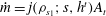
Isentropic patterns are separated by so-called transitional isentropic patterns. Isentropes corresponding to transitional isentropic patterns are sketched in figure 3(a,b) for a constant value of the total enthalpy (the same used in the computation of figure 1). The limiting curve for $\mathscr{S}_{\text{}}^{NI}/\mathscr{S}_{1}^{NC}$ transition includes a simple ( $J\neq 0$ ) high-density sonic point and a non-simple ( $J=0$ ) low-density sonic point. The latter splits into two distinct simple sonic points (isentropic pattern $\mathscr{S}_{1}^{NC}$ ) if the stagnation density is slightly decreased. Next, when ${\it\rho}_{s_{3}}c({\it\rho}_{s_{3}},s)={\it\rho}_{s_{1}}c({\it\rho}_{s_{1}},s)$ the mass flux function has two distinct global maxima and transition $\mathscr{S}_{1}^{NC}/\mathscr{S}_{2}^{NC}$ occurs. With decreasing stagnation density, the two high-density sonic points approach each other and eventually merge in the transitional isentropic flow $\mathscr{S}_{2}^{NC}/\mathscr{S}_{3}^{NC}$ . Finally, the limiting curve for $\mathscr{S}_{3}^{NC}/\mathscr{S}_{\text{}}^{I}$ transition intersects the locus $J=0$ at its minimum ( $J=0$ and ${\it\Lambda}=0$ simultaneously).

Figure 3. Variation of (a) Mach number and (b) mass flux function with density for transitional isentropic flows, computed from the polytropic van der Waals model with $c_{v}/R=50$ . The total enthalpy is constant and equal to the value employed in the computation of figure 1.

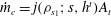
Figure 4. Thermodynamic map of stagnation states related to each isentropic pattern, computed from the van der Waals polytropic model with $c_{v}/R=50$ . Curves labelled $s=s_{vle}$ and $s=s_{{\it\tau}}$ represent the isentropes tangent to the vapour dome and to the ${\it\Gamma}=0$ locus, respectively.

The value of the total enthalpy that was used for the computation of figures 1 and 3 is such that all different isentropic patterns possibly arise. By varying the total enthalpy and gathering the values of stagnation states corresponding to transitional isentropic patterns, one ultimately obtains a thermodynamic map as shown, e.g. for the $P$ – $v$ diagram in figure 4. The map in figure 4 allows one to determine the isentropic pattern resulting from a given set of stagnation thermodynamic conditions. Due to the assumption of single-phase flows, the thermodynamic region of interest is bounded by the saturated vapour boundary if $s<s_{vle}$ . In this case, we can consider the vapour-phase portion of the isentrope and, in spite of the possibility that the region ${\it\Gamma}<0$ is crossed, pattern $\mathscr{S}_{\text{}}^{I}$ necessarily occurs. Note that this is a major difference compared to non-classical unsteady flows. In a steady flow, non-classical effects are due to the possibly non-monotone evolution of the Mach number, which arises in the nearly sonic or supersonic regime. Therefore, the corresponding stagnation states must be located at density values higher than those associated with the negative- ${\it\Gamma}$ region. If $s_{vle}<s<s_{{\it\tau}}$ , where $s_{{\it\tau}}$ denotes the isentrope tangent to the locus ${\it\Gamma}=0$ , each class of isentropic flow can be observed depending on the stagnation state. In the direction of increasing density, patterns $\mathscr{S}_{\text{}}^{I}$ , $\mathscr{S}_{3}^{NC}$ , $\mathscr{S}_{2}^{NC}$ , $\mathscr{S}_{1}^{NC}$ and $\mathscr{S}_{\text{}}^{NI}$ are encountered. With increasing values of $s$ , the region of stagnation states leading to non-classical isentropic patterns shrinks and the corresponding transitional curves ultimately coincide in a single thermodynamic state when $s=s_{{\it\tau}}$ . Along isentropes featuring $0<{\it\Gamma}<1$ , the Mach number may exhibit a non-monotone profile in the supersonic regime, because $J>0$ if ${\it\Gamma}<1$ and $M$ is sufficiently large. Accordingly, either $\mathscr{S}_{\text{}}^{NI}$ or $\mathscr{S}_{\text{}}^{I}$ is possible depending on the stagnation state. The transitional locus $\mathscr{S}_{\text{}}^{NI}/\mathscr{S}_{\text{}}^{I}$ is constructed in the same way as $\mathscr{S}_{3}^{NC}/\mathscr{S}_{\text{}}^{I}$ , i.e. it comprises all stagnation states corresponding to isentropes that intersect the locus $J=0$ at its minimum (with the difference that for $\mathscr{S}_{\text{}}^{NI}/\mathscr{S}_{\text{}}^{I}$ said minimum is supersonic). If ${\it\Gamma}>1$ everywhere along the reference isentrope, the Mach number is a monotone decreasing function of the density and pattern $\mathscr{S}_{\text{}}^{I}$ only can take place.

The identification of the different types of isentropic flow behaviour is essential prior to the construction of general solutions to nozzle flows, which possibly include shock waves. Indeed, smooth branches of any quasi-1D flow can be associated locally with an isentropic pattern. The entropy jump across shock waves results in a shift of the pertinent isentropic curve and can possibly result in the qualitative modification of the flow behaviour, i.e. in a transition of the isentropic pattern. The second law of thermodynamics dictates the direction in which this process can possibly occur. The stagnation density decreases with increasing entropy at constant enthalpy,

(2.9) $$\begin{eqnarray}\displaystyle \left({\displaystyle \frac{\partial {\it\rho}}{\partial s}}\right)_{h}=-{\displaystyle \frac{{\it\rho}T(1+G)}{c^{2}}}<0, & & \displaystyle\end{eqnarray}$$

where $G=v(\partial P/\partial e)_{v}$ is the Grüneisen parameter, which we assume to be positive here throughout. Menikoff & Plohr (Reference Menikoff and Plohr1989) discussed the assumption of $G>0$ for real materials, which is implied by a positive value of the coefficient of thermal expansion, a condition fulfilled by most fluids of interest (with the relevant exception of water at 0 $^{\circ }$ C and 1 bar, see Bethe Reference Bethe1942). Therefore, with reference to figure 3(a,b), transitions of the isentropic pattern occur in the direction of increasing entropy as follows:

(2.10) $$\begin{eqnarray}\displaystyle \mathscr{S}_{}^{NI}\rightarrow \mathscr{S}_{1}^{NC}\rightarrow \mathscr{S}_{2}^{NC}\rightarrow \mathscr{S}_{3}^{NC}\rightarrow \mathscr{S}_{}^{I}. & & \displaystyle\end{eqnarray}$$

Evidently, the transition is not required to occur between two consecutive isentropic patterns (e.g.  $\mathscr{S}_{\text{}}^{NI}\rightarrow \mathscr{S}_{2}^{NC}$ or $\mathscr{S}_{3}^{NC}\rightarrow \mathscr{S}_{\text{}}^{I}$ are admissible transitions). One of the most relevant consequences of the entropy rise across a shock wave is the possible change in the number of sonic points, for the phase planes featuring one only and three sonic points are structurally different, see § 2.2. The number of sonic points may either decrease (following an e.g.  $\mathscr{S}_{1}^{NC}\rightarrow \mathscr{S}_{3}^{NC}$ transition), or increase (e.g.  $\mathscr{S}_{\text{}}^{NI}\rightarrow \mathscr{S}_{2}^{NC}$ ). In addition, from previous investigations it was inferred that non-classical flow fields are associated with reservoir conditions of type $\mathscr{S}_{1}^{NC}$ and $\mathscr{S}_{2}^{NC}$ . The present analysis suggests that non-classical flow configurations are expected also from reservoir conditions featuring a single sonic point, namely $\mathscr{S}_{\text{}}^{NI}$ , because of the possible transition $\mathscr{S}_{\text{}}^{NI}\rightarrow \mathscr{S}_{1}^{NC}$ , $\mathscr{S}_{2}^{NC}$ . The latter claim is confirmed in the following section.

3.1 Functioning regimes: overview

We will investigate quasi-1D steady nozzle flows by examining the dependence of the flow field on the ambient pressure $P_{a}$ , or similarly on the ambient to reservoir pressure ratio ${\it\beta}=P_{a}/P_{r}$ , for given reservoir conditions (subscript $r$ will be used to denote reservoir quantities). When the range $0<{\it\beta}\leqslant 1$ is spanned, a specific sequence of solutions is observed, which together delineate the so-called functioning regime, to be referred to as $\mathscr{R}$ in the following. Any functioning regime is conveniently represented in terms of limiting and intermediate solutions. We formally define as intermediate a solution whose qualitative structure remains unaltered under arbitrary small variations of the ambient pressure. Conversely, a solution is a limiting one if an arbitrary small variation of the ambient pressure produces modifications to its qualitative structure, that is, limiting solutions are isolated solutions of the boundary value problem. Correspondingly, a set of limiting values of the ambient pressure is defined; each pressure value is associated with a limiting flow. Intermediate solutions are observed whenever the ambient pressure lies between two consecutive limiting values. Generally speaking, the qualitative structure of a solution is characterized by the existence and the possible sequence of shock waves. This will be made clear in the subsequent discussion.

Table 2. Summary of the functioning regimes in a converging–diverging nozzle produced by different isentropic patterns of the reservoir conditions.

It is anticipated here, for the understanding of the following treatment, that starting from five different isentropic patterns associated with the reservoir conditions, as many as 10 different functioning regimes have been singled out in the present analysis, and they are gathered in the six classes in table 2. Two classical functioning regimes are introduced: the ideal one $\mathscr{R}_{\text{}}^{I}$ in § 3.2 and the non-ideal one $\mathscr{R}_{\text{}}^{NI}$ in § 3.7, which are produced by reservoir conditions of type $\mathscr{S}_{\text{}}^{I}$ and $\mathscr{S}_{\text{}}^{NI}$ , respectively. These two regimes are characterized by the possibility of observing a classical compression shock in the divergent section. Regime $\mathscr{S}_{\text{}}^{NI}$ further allows for a non-monotone evolution of the Mach number in the supersonic divergent section. Reservoir conditions featuring pattern $\mathscr{S}_{3}^{NC}$ produce the non-classical regime $\mathscr{R}_{3}^{NC}$ described in § 3.3, which features non-monotonic Mach number profile in the subsonic regime, in both the converging and diverging sections. As for non-classical functioning regimes associated with patterns $\mathscr{S}_{1}^{NC}$ and $\mathscr{S}_{2}^{NC}$ , two general classes may be delineated, namely $\mathscr{R}_{1}^{NC}$ and $\mathscr{R}_{2}^{NC}$ , both possibly featuring rarefaction shocks. In the case of the $\mathscr{R}_{2}^{NC}$ flows detailed in § 3.4, the rarefaction shock is sonic on the upstream side and it is located in the converging section of the nozzle. In flows of type $\mathscr{R}_{1}^{NC}$ , the rarefaction shock is sonic on the downstream side and it lies in the diverging section of the nozzle, see § 3.5. A further grouping is outlined, that is sub-classes $a,b$ and $c$ of $\mathscr{R}_{1}^{NC}$ and $\mathscr{R}_{2}^{NC}$ , which are defined in § 3.6 according to the occurrence of shock splitting. Finally, it is shown in § 3.8 that a non-classical functioning regime, namely $\mathscr{R}_{0}^{NC}$ , is produced by $\mathscr{S}_{\text{}}^{NI}$ reservoir conditions which are characterized by the occurrence of a single sonic point.

Functioning regimes will be discussed in the order of increasing number of possible transition of the isentropic pattern (see the ordering in (2.10)), starting from $\mathscr{S}_{\text{}}^{I}$ reservoir conditions, where no transition can take place, up to $\mathscr{S}_{\text{}}^{NI}$ reservoir conditions, from where all transitions are possible.

Figure 5. Exemplary limiting (- - - -) and intermediate (——) flows of type $\mathscr{R}_{\text{}}^{I}$ , computed from the van der Waals polytropic model with $c_{v}/R=50$ . (a) Density solutions, scaled to reservoir density ${\it\rho}_{r}$ ; (b) Mach number solutions. Reservoir conditions: $P_{r}=10P_{c}$ , $v_{r}=10v_{c}$ .

3.2 Functioning regime $\mathscr{R}_{\text{}}^{I}$

The layout of the possible flow configurations produced by $\mathscr{S}_{\text{}}^{I}$ reservoir conditions corresponds to the textbook case of an ideal gas with constant specific heats, see for instance Thompson (Reference Thompson1988). The main results are reported here for reference and are extended to a general, non-ideal thermodynamic description of the fluid. Limiting and intermediate flows are reported in figure 5. Flows of type $\mathscr{R}_{}^{I}(1)$ are completely subsonic and are characterized by increasing mass flow rate with decreasing ambient pressure. Limiting solution $\mathscr{R}_{}^{I}(1{-}2)$ determines the so-called choking condition, because the throat is sonic and a further decrease of the ambient pressure has no influence on the mass flow rate. Let ${\dot{m}}_{max}$ denote the maximum mass flow rate dischargeable by the nozzle and ${\dot{m}}_{s_{\text{}}}$ the mass flow rate in the choked condition; then

(3.1) $$\begin{eqnarray}\displaystyle {\dot{m}}_{max}={\dot{m}}_{s_{\text{}}}={\dot{m}}_{c}(s_{r},h^{t}), & & \displaystyle\end{eqnarray}$$

where the critical mass flow rate ${\dot{m}}_{c}$ is defined by (2.7) and $s_{r}$ is the reservoir entropy. If ${\it\beta}<{\it\beta}_{1{-}2}$ , where ${\it\beta}_{1{-}2}$ is the pressure ratio corresponding to limiting solution $\mathscr{R}_{}^{I}(1{-}2)$ , the flow is choked and subsonic to supersonic transition occurs at the throat. Intermediate flows $\mathscr{R}_{}^{I}(2)$ include a compression shock wave in the diverging section of the nozzle. It can be shown that the entropy jump across the shock wave increases with decreasing ambient pressure. The mass balance equation, evaluated on the outlet section, provides an implicit definition for $s_{e}(P_{e};{\dot{m}},h^{t},A_{e})$ , where subscript $e$ denotes the exit quantities. Thus, if the flow is choked, we obtain

(3.2) $$\begin{eqnarray}\displaystyle {\displaystyle \frac{\text{d}s_{e}}{\text{d}P_{e}}}={\displaystyle \frac{M_{e}^{2}-1}{{\it\rho}_{e}T_{e}(M_{e}^{2}G_{e}+1)}}. & & \displaystyle\end{eqnarray}$$

Note that if the outflow is subsonic, as is the case for solutions of type $\mathscr{R}_{}^{I}(2)$ , then $P_{e}=P_{a}$  and $\text{d}s_{e}/\text{d}P_{e}=\text{d}s_{e}/\text{d}P_{a}$ in the corresponding range of ${\it\beta}$ . In addition, by combining the jump relations and the differential relations for quasi-1D flows, one has

(3.3) $$\begin{eqnarray}\displaystyle {\displaystyle \frac{\text{d}x_{s}}{\text{d}s_{B}}}={\displaystyle \frac{A}{A^{\prime }}}{\displaystyle \frac{{\it\rho}_{A}T_{B}}{[P]}}\left({\displaystyle \frac{1}{M_{B}^{2}}}+{\displaystyle \frac{[v]}{2v_{B}}}G_{B}\right)\left[\left({\displaystyle \frac{1}{M_{B}^{2}}}-1\right){\displaystyle \frac{v_{B}}{v_{A}}}+{\displaystyle \frac{1}{2}}\right]^{-1}, & & \displaystyle\end{eqnarray}$$

where $x_{s}$ is the location of the shock wave and $[X]=X_{B}-X_{A}$ is the jump between a quantity evaluated at the post-shock state (subscript $B$ ) and at the pre-shock state (subscript $A$ ). Given that $M_{B}<1$ , the last two terms are positive (the condition $2v_{B}+[v]G_{B}=0$ is the singularity that limits the maximum possible density increase across compression shocks, see Kluwick Reference Kluwick2001). Hence, a compression shock in the diverging section of the nozzle moves downstream with increasing post-shock entropy, which, in turn, corresponds to decreasing values of the ambient pressure, as is seen by (3.2) together with $s_{e}=s_{B}$ and $P_{e}=P_{a}$ . Ultimately, the shock wave reaches the exit section, see limiting flow $\mathscr{R}_{}^{I}(2{-}3)$ . Flows of type $\mathscr{R}_{}^{I}(3)$ have supersonic exit conditions and may exhibit an over-expanded or under-expanded jet outside of the nozzle if ${\it\beta}\neq {\it\beta}_{3}$ , where ${\it\beta}_{3}$ corresponds to the exit pressure of solution $\mathscr{R}_{}^{I}(3)$ .

3.3 Functioning regime $\mathscr{R}_{3}^{NC}$

If the reservoir conditions correspond to isentropic pattern $\mathscr{S}_{3}^{NC}$ , the Mach number does not increase monotonically through a subsonic expansion. The related functioning regime is a non-classical one, since $J>0$ in a subsonic flow requires ${\it\Gamma}<0$ , and it is denoted by $\mathscr{R}_{3}^{NC}$ . Limiting and intermediate flows of regime $\mathscr{R}_{3}^{NC}$ are sketched in figure 6. The layout and the general properties of the solutions are as described above for the case $\mathscr{R}_{\text{}}^{I}$ , except for a pronounced subsonic peak in the Mach number. This appears as a steeper expansion or compression in the density solutions. In addition, contrary to the ideal case, in flows of type $\mathscr{R}_{3}^{NC}(2)$ the Mach number may also increase downstream of the shock wave in the divergent section. If, however, transition $\mathscr{S}_{2}^{NI}\rightarrow \mathscr{S}_{\text{}}^{I}$ occurs in passing through the shock wave, the Mach number will necessarily decrease up to the exit section, as in the exemplary solution $\mathscr{R}_{3}^{NC}(2)$ reported in figure 6.

Figure 6. Exemplary limiting (- - - -) and intermediate (——) flows of type $\mathscr{R}_{3}^{NC}$ , computed from the van der Waals polytropic model with $c_{v}/R=50$ . (a) Density solutions, scaled to reservoir density ${\it\rho}_{r}$ ; (b) Mach number solutions. Reservoir conditions: $P_{r}=1.1427P_{c}$ , $v_{r}=0.8058v_{c}$ .

3.4 Functioning regimes $\mathscr{R}_{2}^{NC}$

When the isentropic pattern of the reservoir conditions exhibits three sonic points, the layout of the possible flow fields is considerably more complex. Here we discuss regimes of type $\mathscr{R}_{2}^{NC}$ , which exhibit a rarefaction shock wave in the converging section of the nozzle and can originate from reservoir conditions of type $\mathscr{S}_{2}^{NC}$ , see table 2. Three possible configurations are admissible and detailed in § 3.6: $\mathscr{R}_{2a}^{NC}$ , $\mathscr{R}_{2b}^{NC}$ and $\mathscr{R}_{2c}^{NC}$ . Here, the regime $\mathscr{R}_{2a}^{NC}$ in figure 7 – corresponding to the Type-2 flows of Cramer & Fry (Reference Cramer and Fry1993) – is presented to describe common features to all $\mathscr{R}_{2}^{NC}$ regimes.

Inspection of figure 7 reveals that flows such as $\mathscr{R}_{2a}^{NC}(2)$ , including a single compression shock in the diverging section of the nozzle, exist for a very limited range of ambient pressure. This shock, owing to the non-monotone dependence of the Mach number on the density, ultimately has sonic upstream state ( ${\it\rho}={\it\rho}_{s_{2}}$ ), see limiting solution $\mathscr{R}_{2a}^{NC}(2{-}3)$ , and cannot exist further downstream. Shocks with upstream sonic state will be referred to as pre-sonic shocks in the following.

If the ambient pressure is slightly reduced below ${\it\beta}={\it\beta}_{2{-}3}$ , the necessary entropy rise is carried by a double-shock configuration, in which the leading wave is a rarefaction shock and the trailing wave is a pre-sonic compression shock. The trailing shock is formed because the flow downstream of the rarefaction shock becomes sonic when ${\it\rho}={\it\rho}_{s_{2}}$ in the local isentropic pattern, which remains of type $\mathscr{S}_{2}^{NC}$ (i.e. no transition occurs across the leading shock). Intermediate flows of type $\mathscr{R}_{2a}^{NC}(2)$ and $\mathscr{R}_{2a}^{NC}(3)$ are sonic at the throat (sonic condition ${\it\rho}_{s_{1}}$ ). Therefore, the nozzle is choked in the corresponding range of ambient pressure, with a constant value of the mass flow rate denoted as ${\dot{m}}_{s_{1}}$ . Moreover, the simultaneous shift upstream of the rarefaction shock and downstream of the pre-sonic compression shock, in accordance with relation (3.3), makes it possible to satisfy the overall increasing entropy jump in a choked flow as the ambient pressure is decreased, cf. (3.2). Eventually, the leading shock wave has sonic upstream state and it is located exactly at the throat section, see limiting solution $\mathscr{R}_{2a}^{NC}(3{-}4)$ .

Figure 7. Exemplary limiting (- - - -) and intermediate (——) flows of type $\mathscr{R}_{2a}^{NC}$ , computed from the van der Waals polytropic model with $c_{v}/R=50$ . (a) Density solutions, scaled to reservoir density ${\it\rho}_{r}$ ; (b) Mach number solutions; (c) enlargement of (b) including only flows from 2 to 4; (d) enlargement of (b) including only flows from 4 to 7. Reservoir conditions: $P_{r}=1.1300P_{c}$ , $v_{r}=0.7710v_{c}$ .

A rarefaction shock with sonic upstream state can also exist ahead of the throat. If ${\it\beta}_{4{-}5}<{\it\beta}<{\it\beta}_{3{-}4}$ , the mass flow rate increases with decreasing ambient pressure and sonic condition ${\it\rho}_{s_{1}}$ occurs upstream of the throat. Trajectories such as $\mathscr{R}_{2a}^{NC}(4)$ can be continued provided a sonic rarefaction shock is inserted at the sonic point. Notably, this shock has the same upstream and downstream states as the leading shock in limiting flow $\mathscr{R}_{2a}^{NC}(3{-}4)$ , albeit in a different location. Downstream of the rarefaction shock, the flow expands up to the throat because of the converging area. Flows of type $\mathscr{R}_{2a}^{NC}(4)$ are subsonic at the throat and therefore the pressure and density increase in the diverging section of the nozzle. Because the local isentropic pattern is $\mathscr{S}_{2}^{NC}$ , a pre-sonic compression shock must be inserted to continue the flow beyond sonic point ${\it\rho}_{s_{2}}$ (this shock is identical to that of limiting solution $\mathscr{R}_{2a}^{NC}(3{-}4)$ ). The mass flow rate can be increased by decreasing ${\it\beta}$ until $M=1$ at the throat, whereby the sonic condition corresponds to the low-density sonic point ${\it\rho}_{s_{3}}$ in the isentrope downstream of the rarefaction shock. This condition determines limiting flow $\mathscr{R}_{2a}^{NC}(4{-}5)$ , in which the pre-sonic rarefaction shock is in its rearmost position. Let $s_{t}$ denote the entropy value downstream of this shock wave and let ${\dot{m}}_{s_{2}}$ be the mass flow rate corresponding to ${\it\beta}={\it\beta}_{4{-}5}$ . Then

(3.4) $$\begin{eqnarray}\displaystyle {\dot{m}}_{max}={\dot{m}}_{s_{2}}={\dot{m}}_{c}(s_{t},h^{t})<{\dot{m}}_{c}(s_{r},h^{t}), & & \displaystyle\end{eqnarray}$$

where the last inequality follows from $(\partial j/\partial s)_{{\it\rho},h^{t}}=-{\it\rho}T(1+G)/\sqrt{2(h^{t}-h)}$ , which gives $(\partial {\dot{m}}_{c}/\partial s)_{h^{t}}<0$ and from the admissibility requirement $s_{t}>s_{r}$ . Note that there exist two different choking conditions in functioning regime $\mathscr{R}_{2a}^{NC}$ , namely ${\it\beta}_{3{-}4}<{\it\beta}<{\it\beta}_{1{-}2}$ ( ${\dot{m}}={\dot{m}}_{s_{1}}$ ) and ${\it\beta}<{\it\beta}_{4{-}5}$ ( ${\dot{m}}={\dot{m}}_{s_{2}}$ ).

Flows such as $\mathscr{R}_{2a}^{NC}(5)$ or $\mathscr{R}_{2a}^{NC}(6)$ admit ordinary compression shock waves in the diverging section of the nozzle. If the shock is sufficiently close to the throat, as in case $\mathscr{R}_{2a}^{NC}(5)$ , the resultant subsonic compression eventually attains a sonic point and a further shock, with sonic upstream state, must be formed to continue the flow. Following Kluwick (Reference Kluwick1993) and Cramer & Fry (Reference Cramer and Fry1993), we will refer to this double compression-shock configuration as a split shock, owing to the analogies with the shock-splitting phenomenon in unsteady flows (see Wendroff Reference Wendroff1972; Menikoff & Plohr Reference Menikoff and Plohr1989; Cramer Reference Cramer and Kluwick1991). According to relation (3.3), if the leading compression shock moves downstream the corresponding entropy jump increases. Indeed, a reduction of the ambient pressure results in a stronger leading shock and in a weaker terminating shock. Ultimately, the entropy rise across the first compression shock is such that, in the downstream flow, the isentropic pattern corresponds to the transitional type $\mathscr{S}_{2}^{NC}/\mathscr{S}_{3}^{NC}$ . Thus, in the limiting flow $\mathscr{R}_{2a}^{NC}(5{-}6)$ the trailing sonic shock wave has vanishing strength.

If ${\it\beta}<{\it\beta}_{5{-}6}$ , a single non-sonic compression shock occurs, because the post-shock isentropic pattern is either $\mathscr{S}_{3}^{NC}$ or $\mathscr{S}_{\text{}}^{I}$ . Hence, if a compression shock forms sufficiently far downstream of the throat, as is the case in flows of type $\mathscr{R}_{2a}^{NC}(6)$ , the post-shock isentrope no longer contains the sonic point required for the existence of the sonic compression shock. As in previous regimes, with decreasing ambient pressure the shock wave moves downstream in the diverging section of the nozzle and eventually attains the exit section in limiting flow $\mathscr{R}_{2a}^{NC}(6{-}7)$ . If ${\it\beta}<{\it\beta}_{6{-}7}$ , no shock waves exist downstream of the throat and the outflow is supersonic. The major difference with respect to flows including a single sonic point is that flows such as $\mathscr{R}_{2a}^{NC}(7)$ , having arbitrarily large exit Mach number, must include a pre-sonic rarefaction shock upstream of the throat.

3.5 Functioning regimes $\mathscr{R}_{1}^{NC}$

Regimes of type $\mathscr{R}_{1}^{NC}$ , including regimes $\mathscr{R}_{1a}^{NC}$ , $\mathscr{R}_{1b}^{NC}$ and $\mathscr{R}_{1c}^{NC}$ described in § 3.6, exhibit a rarefaction shock wave in the diverging section of the nozzle and can originate from reservoir conditions of type $\mathscr{S}_{1}^{NC}$ or $\mathscr{S}_{2}^{NC}$ , see table 2. The regime $\mathscr{R}_{1a}^{NC}$ in figure 8 – corresponding to Type-1 flows of Cramer & Fry (Reference Cramer and Fry1993) – is now presented to outline all regimes of type $\mathscr{R}_{1}^{NC}$ .

Figure 8. Exemplary limiting (- - - -) and intermediate (——) flows of type $\mathscr{R}_{1a}^{NC}$ , computed from the van der Waals polytropic model with $c_{v}/R=50$ . (a) Density solutions, scaled to reservoir density ${\it\rho}_{r}$ ; (b) Mach number solutions; (c) enlargement of (b) including only flows from 2 to 4; (d) enlargement of (b) including only flows from 4 to 6. Reservoir conditions: $P_{r}=1.1453P_{c}$ , $v_{r}=0.7600v_{c}$ .

With reference to figure 8, flows $\mathscr{R}_{1a}^{NC}(1)$ , $\mathscr{R}_{1a}^{NC}(2)$ and $\mathscr{R}_{1a}^{NC}(3)$ are qualitatively similar to $\mathscr{R}_{2a}^{NC}(1)$ , $\mathscr{R}_{2a}^{NC}(2)$ and $\mathscr{R}_{2a}^{NC}(3)$ , respectively, discussed in the previous section. Differently from $\mathscr{R}_{2a}^{NC}(3)$ , the rarefaction shock of intermediate flow $\mathscr{R}_{1a}^{NC}(3)$ becomes sonic on the downstream side (post-sonic shock) when ${\it\beta}={\it\beta}_{3{-}4}$ . Rarefaction shocks cannot exist ahead of this limiting sonic shock. Thus, in contrast to $\mathscr{R}_{2a}^{NC}$ flows, functioning regime $\mathscr{R}_{1a}^{NC}$ exhibits a unique sonic condition at the throat, corresponding to the high-density sonic point ${\it\rho}_{s1}$ . Accordingly,

(3.5) $$\begin{eqnarray}\displaystyle {\dot{m}}_{max}={\dot{m}}_{s_{\text{}}}={\dot{m}}_{c}(s_{r},h^{t}), & & \displaystyle\end{eqnarray}$$

where ${\dot{m}}_{s_{\text{}}}$ is the mass flow rate discharged when ${\it\beta}<{\it\beta}_{1{-}2}$ . If ${\it\beta}<{\it\beta}_{3{-}4}$ , the flow expands downstream of the limiting rarefaction shock and two different shock configurations are possible, similarly to functioning regime $\mathscr{R}_{2a}^{NC}$ . Compression waves in the neighbourhood of the limiting rarefaction shock occur in the form of a split shock, see intermediate flow $\mathscr{R}_{1a}^{NC}(4)$ . The split-shock configuration ultimately vanishes because of the disintegration of the sonic compression shock, as a result of the shift in the isentrope across the leading compression shock. If ${\it\beta}_{5{-}6}<{\it\beta}<{\it\beta}_{4{-}5}$ , a single non-sonic shock is formed downstream of the limiting rarefaction shock, for the subsequent flow remains subsonic. Finally, flows such as $\mathscr{R}_{1a}^{NC}(6)$ , expanding to arbitrarily low densities and arbitrarily large Mach numbers, are realizable provided that a rarefaction shock with sonic downstream state is inserted into the diverging section of the nozzle.

The two non-classical functioning regimes that we have described so far, namely $\mathscr{R}_{1a}^{NC}$ and $\mathscr{R}_{2a}^{NC}$ , are in fact the Type-1 and Type-2 flows introduced by Cramer & Fry (Reference Cramer and Fry1993), respectively, and have been introduced to describe the features of $\mathscr{R}_{1}^{NC}$ and $\mathscr{R}_{2}^{NC}$ flows, respectively. In the following section we show that a further classification can be formulated according to the mechanism by which the split shock turns into the single-shock configuration.

3.6 On the split-shock/single-shock transition: sub-classes $\mathscr{R}_{a}^{NC}$ , $\mathscr{R}_{b}^{NC}$ and $\mathscr{R}_{c}^{NC}$

In order to investigate the different scenarios for the split-shock formation and eventual disintegration, it is instructive to examine the quantity

(3.6) $$\begin{eqnarray}\displaystyle {\it\Psi}=j({\it\rho};s,h^{t})-j^{\ast }({\it\rho};s), & & \displaystyle\end{eqnarray}$$

where $j^{\ast }$ is the mass flux corresponding to a post-sonic compression shock, which is the difference between the slopes of the Rayleigh lines for a shock with total enthalpy $h^{t}$ and for a post-sonic compression shock, both centred on the thermodynamic state identified by ${\it\rho}$ and $s$ . Note that $j^{\ast }$ and, in turn, ${\it\Psi}$ are defined only if a post-sonic compression shock can originate from the given pre-shock state. By analysing the properties of non-convex shock adiabats, it is possible to prove (see e.g. Kluwick Reference Kluwick2001) that, if a post-sonic compression shock centred on a given pre-shock state exists and is admissible, then it is unique.

Figure 9. Isolines of $h^{t}$ in the ${\it\Psi}$ – ${\it\rho}$ diagram corresponding to the exemplary isentrope $s=s(1.0923P_{c},v_{c})$ , as computed from the van der Waals polytropic model with $c_{v}/R=50$ . The range of densities is restricted to those where $j^{\ast }$ is defined, i.e. where a post-sonic compression shock can possibly originate. Two additional curves are plotted: the sonic locus $M=1$ and the sonic shock disintegration (SD) locus, gathering the pre-shock states corresponding to a shock wave with downstream isentropic pattern $\mathscr{S}_{2}^{NC}/\mathscr{S}_{3}^{NC}$ . The SD locus intersects the sonic locus at point $P_{2}$ . The curve passing through point $P_{2}$ corresponds to the transitional isentropic pattern $\mathscr{S}_{2}^{NC}/\mathscr{S}_{3}^{NC}$ . On the other hand, the curve passing through point $P_{1}$ ( $M=1$ and ${\it\Psi}=0$ ) corresponds to the transitional isentropic pattern $\mathscr{S}_{\text{}}^{NI}/\mathscr{S}_{1}^{NC}$ .

Figure 9 shows exemplary isolines of $h^{t}$ in the ${\it\Psi}$ – ${\it\rho}$ plane of a given isentrope. In this diagram, the abscissa spans the range of densities where a post-sonic compression shock is admissible. Two relevant curves are plotted, namely the sonic locus and the sonic shock disintegration (SD) locus. States located at densities lower than those on the sonic locus represent supersonic, and therefore candidate pre-shock states of admissible shock waves. By combining (3.3) with the well-known differential relations for quasi-1D isentropic flows, it is easy to show that the entropy jump increases with decreasing density of the candidate pre-shock state, provided that the shock wave is compressive. Ultimately, when the pre-shock state occurs on the SD locus, the post-shock isentropic pattern corresponds to the transitional type $\mathscr{S}_{2}^{NC}/\mathscr{S}_{3}^{NC}$ .

To aid understanding of the following analysis, the possible compression-wave configurations in the thermodynamic region of interest in this work have been sketched in the $P$ – $v$ plane, see figure 10. Here ${\it\rho}_{A}$ denotes the density at the selected pre-shock state $A$ and ${\it\rho}_{SD}$ represents the density corresponding to the intersection between ${\it\Psi}({\it\rho};s,h^{t})$ and the SD locus. Split shocks occur when ${\it\Psi}<0$ and ${\it\rho}_{A}>{\it\rho}_{SD}$ , because, along the isentropic compression resulting from shock $A{-}B$ , sonic point $S$ is encountered and a further shock wave is required to continue the flow. Note that state $S$ is necessarily embedded in the region ${\it\Gamma}<0$ , for the curvatures of the shock adiabat and of the isentrope have the same sign in the $P$ – $v$ plane at a sonic point (see, e.g. Menikoff & Plohr Reference Menikoff and Plohr1989).

Figure 10. Qualitative chart illustrating compression waves that bridge the negative- ${\it\Gamma}$ region: $H_{A}$ and $H_{S}$ are shock adiabats from points $A$ and $S$ , respectively; $R_{A}$ and $R_{S}$ are Rayleigh lines; $I_{B}$ is an isentrope. Case ${\it\Psi}<0$ , ${\it\rho}_{A}>{\it\rho}_{SD}$ : split-shock composed of shock $A{-}B$ , isentropic compression along $I_{B}$ up to sonic point $S$ and sonic shock $S{-}C$ . Case ${\it\Psi}<0$ , ${\it\rho}_{A}<{\it\rho}_{SD}$ : shock $A{-}B$ followed by isentropic compression along $I_{B}$ . Case ${\it\Psi}=0$ : the Rayleigh line $R_{A}$ of shock $A{-}C$ is tangent to the shock adiabat $H_{A}$ at the intermediate sonic step $S$ ; this shock can be seen as a unique non-sonic shock or as the composition of post-sonic shock $A{-}S$ and pre-sonic shock $S{-}C$ . Case ${\it\Psi}>0$ : single shock $A{-}B$ ; the Rayleigh line $R_{A}$ bridges the concave-down region of $H_{A}$ .

There exist two different mechanisms by which the split shock turns into an ordinary non-sonic shock. In the first case, the transition takes place when state $A$ crosses the SD locus and the sonic shock disintegrates. As a result, if ${\it\Psi}<0$ and ${\it\rho}_{A}<{\it\rho}_{SD}$ , sonic point $S$ is no longer encountered in the isentropic compression downstream of shock $A{-}B$ . The split-shock/single-shock transition is also accomplished when ${\it\Psi}$ changes sign. As ${\it\Psi}$ goes to zero from below, a weaker isentropic compression and a stronger terminating shock are generated. When ${\it\Psi}=0$ , state $B$ and sonic point $S$ coincide, i.e. the intermediate isentropic compression vanishes. In this case, the leading shock $A{-}B$ and the trailing shock $S{-}C$ merge in the single large-amplitude shock $A{-}C$ . If ${\it\Psi}>0$ an ordinary shock occurs, because the Rayleigh line completely bridges, without touching, the region where the shock adiabat $H_{A}$ is concave down (inflection points of the shock adiabat nearly coincide with the intersections between the shock adiabat and the ${\it\Gamma}=0$ locus, see for instance Kluwick Reference Kluwick2001).

Figure 11. Exemplary limiting (- - - -) and intermediate (——) flows of type $\mathscr{R}_{2b}^{NC}$ , computed from the van der Waals polytropic model with $c_{v}/R=50$ . (a) Density solutions, scaled to reservoir density ${\it\rho}_{r}$ ; (b) Mach number solutions. Reservoir conditions: $P_{r}=1.2824P_{c}$ , $v_{r}=0.7863v_{c}$ .

We now examine the different configuration reported in figure 9. Curves such as $a$ display ${\it\Psi}<0$ ; the split-shock configuration is formed and eventually vanishes when the pre-shock state crosses the SD locus. We will refer to functioning regimes featuring this kind of split-shock/single-shock transition as the sub-class $\mathscr{R}_{a}^{NC}$ , which includes $\mathscr{R}_{1a}^{NC}$ and $\mathscr{R}_{2a}^{NC}$ . The curve labelled $b$ in figure 9 exhibits a zero with $\text{d}{\it\Psi}/\text{d}{\it\rho}<0$ . In this case, by decreasing the pre-shock density, the two compression shocks in the split-shock configuration merge in a single large-amplitude shock. We will refer to functioning regimes featuring this kind of split-shock/single-shock transition as the sub-class $\mathscr{R}_{b}^{NC}$ ( $\mathscr{R}_{1b}^{NC}$ and $\mathscr{R}_{2b}^{NC}$ ). Figure 11 reports the layout of limiting and intermediate flows corresponding to the exemplary case $\mathscr{R}_{2b}^{NC}$ . The limiting flow corresponding to the overlapping of the compression shocks is $\mathscr{R}_{2b}^{NC}(5{-}6)$ . It is noticeable that the split-shock/single-shock transition of $\mathscr{R}_{b}^{NC}$ regimes is qualitatively similar to the transition predicted by the isentropic theory, i.e. if we were to neglect the entropy rise across shock waves (see Cramer & Fry Reference Cramer and Fry1993; Kluwick Reference Kluwick1993).

In addition to $\mathscr{R}_{a}^{NC}$ and $\mathscr{R}_{b}^{NC}$ sub-classes, we introduce the sub-class $\mathscr{R}_{c}^{NC}$ ( $\mathscr{R}_{1c}^{NC}$ and $\mathscr{R}_{2c}^{NC}$ ) of the functioning regimes in which a double split-shock/single-shock transition occurs. This is expected when the stagnation conditions are such that ${\it\Psi}$ has two zeros, as is the case in curves of type $c$ in figure 9. The layout of the limiting and intermediate flows for the exemplary case $\mathscr{R}_{1c}^{NC}$ is sketched in figure 12. When the high-density zero of ${\it\Psi}$ ( $\text{d}{\it\Psi}/\text{d}{\it\rho}<0$ ) is encountered, the two compression shocks merge, see limiting flow $\mathscr{R}_{1c}^{NC}(4{-}5)$ . The reverse process occurs in limiting solution $\mathscr{R}_{1c}^{NC}(5{-}6)$ , because the pre-shock density corresponds to the low-density zero of ${\it\Psi}$ , where $\text{d}{\it\Psi}/\text{d}{\it\rho}>0$ . By further decreasing the pre-shock density, the split shock ultimately vanishes as in $\mathscr{R}_{a}^{NC}$ regimes, i.e. the sonic shock disintegrates.

Figure 12. Exemplary limiting (- - - -) and intermediate (——) flows of type $\mathscr{R}_{1c}^{NC}$ , computed from the van der Waals polytropic model with $c_{v}/R=50$ . (a) Density solutions, scaled to reservoir density ${\it\rho}_{r}$ ; (b) Mach number solutions. Reservoir conditions: $P_{r}=1.2102P_{c}$ , $v_{r}=0.7542v_{c}$ .

Figure 13. Exemplary limiting (- - - -) and intermediate (——) flows of type $\mathscr{R}_{\text{}}^{NI}$ , computed from the van der Waals polytropic model with $c_{v}/R=50$ . (a) Density solutions, scaled to reservoir density ${\it\rho}_{r}$ ; (b) Mach number solutions. Reservoir conditions: $P_{r}=1.7355P_{c}$ , $v_{r}=0.6532v_{c}$ .

3.7 Functioning regime $\mathscr{R}_{\text{}}^{NI}$

The layout of the possible flows corresponding to reservoir conditions of type $\mathscr{S}_{\text{}}^{NI}$ depends on the possible shock-induced transitions of the isentropic pattern. First of all, note that rarefaction shocks cannot occur in these flows, as in any other functioning regime produced by reservoir conditions featuring a unique sonic point. This is easily seen by analysing the related mass flux functions or phase planes. However, compression waves near the negative- ${\it\Gamma}$ region may occur either as ordinary non-sonic shocks or in the form of split shocks, according to the slope of the Rayleigh line. The same argument concerning the ${\it\Psi}$ – ${\it\rho}$ diagram could be repeated for this type of nozzle flow. The functioning regime arising from reservoir conditions of type $\mathscr{S}_{\text{}}^{NI}$ and corresponding to the case ${\it\Psi}>0$ , which implies that compression shocks occurring in the diverging section of the nozzle are ordinary non-sonic shocks, is denoted as $\mathscr{R}_{\text{}}^{NI}$ . In other words, the possible shock-induced transition of the isentropic pattern does not determine any limiting solutions, so that the layout of limiting and intermediate flows is as shown in figure 13. This functioning regime stands out from $\mathscr{R}_{\text{}}^{I}$ and $\mathscr{R}_{3}^{NC}$ (which have qualitatively similar density solutions) because the Mach number is non-monotone along supersonic branches of isentropic expansions. Moreover, $\mathscr{R}_{\text{}}^{NI}$ is referred to as a non-ideal regime, rather than a non-classical one, because it requires the less restrictive condition ${\it\Gamma}<1$ .

3.8 Functioning regime $\mathscr{R}_{0}^{NC}$

To conclude, we present one additional functioning regime, namely $\mathscr{R}_{0}^{NC}$ , which develops from reservoir states associated with the isentropic pattern $\mathscr{S}_{\text{}}^{NI}$ . Following previous discussion, shocks that bridge the negative- ${\it\Gamma}$ region are expected to split if the isentropic pattern downstream of a generic non-sonic shock exhibits three sonic points and the post-shock state lies between sonic points ${\it\rho}_{s3}$ and ${\it\rho}_{s2}$ . In this case, the resultant subsonic compression eventually encounters sonic point ${\it\rho}_{s2}$ and a further shock is required. The layout of limiting and intermediate flows of the type $\mathscr{R}_{0}^{NC}$ is depicted in figure 14. The splitting mechanism in limiting solution $\mathscr{R}_{0}^{NC}(2{-}3)$ is the same occurring in $\mathscr{R}_{c}^{NC}$ regimes when the low-density zero of ${\it\Psi}$ ( $\text{d}{\it\Psi}/\text{d}{\it\rho}>0$ ) is crossed. Similarly to regimes of type $\mathscr{R}_{a}^{NC}$ , a decrease in ambient pressure results in a weaker sonic shock, which ultimately vanishes when ${\it\beta}={\it\beta}_{3{-}4}$ .

It is remarkable that past qualitative investigations of nozzle flows, based on the simplifying assumption of isentropic flow, i.e. neglecting the entropy rise and the resultant shift in the isentropes across shock waves, led to the erroneous conclusion that non-classical nozzle flows develop exclusively from reservoir states featuring three sonic points.

Figure 14. Exemplary limiting (- - - -) and intermediate (——) flows of type $\mathscr{R}_{0}^{NC}$ , computed from the van der Waals polytropic model with $c_{v}/R=50$ . (a) Density solutions, scaled to reservoir density ${\it\rho}_{r}$ ; (b) Mach number solutions. Reservoir conditions: $P_{r}=1.2315P_{c}$ , $v_{r}=0.7287v_{c}$ .