


1 Introduction
In a coastal environment, sandy particles on the seabed surface will start to move once the shear force exerted by surface waves and currents exceeds critical values. Such motion involves complex fluid–particle and particle–particle interactions and can result in various visible features such as vortex ripples in the low-flow regime, or a flat bed with intensive transport under large stormy waves, i.e. sheet flows (van Rijn Reference van Rijn1993). Increasing evidence from theoretical, experimental and field studies suggests that the physical processes involved in these grain scale interactions often underpin the mechanisms for transport observed on natural beaches. In particular, the size and shape variations of natural sand particles have long been recognized as important factors influencing local sand transport under oscillatory flows. For example, Black & Oldman (Reference Black and Oldman1999) observed wave induced grain size sorting and subsequent effects on sand ripple development on the continental shelf, and Vincent, Stolk & Porter (Reference Vincent, Stolk and Porter1998) and Roos et al. (Reference Roos, Wemmenhove, Hulscher, Hoeijmakers and Kruyt2007) identified spatial variations in the mean grain sizes on the Middelkerke Bank that have clear influences on the sand banks and seabed features along the Belgian coast.
Broadly, grain size influences on transport processes can be classified into two effects. First, for the suspended particles, vertical size sorting and selective transport can lead to very different transport capacity for different size fractions. Especially under oscillatory flows due to surface waves, the strong onshore peak flow under the wave crest can lift a large amount of sand from the bed surface. Once in suspension, the fine fractions take a significant time to settle back to the bed, during which the flow already changes its direction, resulting in enhanced offshore suspended transport, i.e. phase lag effects (Dohmen-Janssen et al. Reference Dohmen-Janssen, Kroekenstoel, Hassan and Ribberink2002). The overall net transport direction for fine sand therefore is often found against the wave propagation direction. In contrast, medium and coarse sands are transported close to the bed by the mean flow, settling during low-velocity phases, and their wave-period averaged net transport tends to be in line with the wave propagation direction (Camenen & Larson Reference Camenen and Larson2006; Hassan & Ribberink Reference Hassan and Ribberink2010; Kranenburg, Hsu & Ribberink Reference Kranenburg, Hsu and Ribberink2014). Second, within the bed, agitation by the oscillatory shear force together with the bed level changes due to bedform migration or bed scour can lead to inverse size gradation (Bagnold Reference Bagnold1954; Legros Reference Legros2002), where coarse fractions rise to the surface, leaving the finer fractions below with very limited mobility. The most noticeable consequence of these armouring and sheltering effects is the shift in transport regime, i.e. a switch from offshore transport towards onshore transport or vice versa (Egiazaroff Reference Egiazaroff1965).
Under oscillatory flows, particle exchange between the bedload and the suspended load is fairly dynamic through competing settling and entrainment effects (Hassan & Ribberink Reference Hassan and Ribberink2005). Therefore, in order to understand the grain size effects, the transport processes within both the suspension layer and the high-concentration bed region need to be examined hand in hand. Yet, most existing model concepts decouple these two regions in some way and largely rely on a single-particle representation of the population of natural sand sizes (van Rijn et al. Reference van Rijn, Ribberink, Werf and Walstra2013). This means that the coupled selective transport in the water column and the sorting/segregation phenomena in the bed are yet to be fully understood (Blondeaux Reference Blondeaux2012). Several series of oscillatory flow experiments have provided detailed measurements of net transport rates, flow hydrodynamics and sediment concentrations for both ‘uniform’ and graded sands in sheet-flow conditions (Ribberink & Al-Salem Reference Ribberink and Al-Salem1994; Ahmed & Sato Reference Ahmed and Sato2003; O’Donoghue & Wright Reference O’Donoghue and Wright2004a ,Reference O’Donoghue and Wright b ; Hassan & Ribberink Reference Hassan and Ribberink2005) as well as above vortex ripples (Ribberink & Al-Salem Reference Ribberink and Al-Salem1994; Fredsøe, Andersen & Sumer Reference Fredsøe, Andersen and Sumer1999; Van der Werf et al. Reference Van der Werf, Doucette, O’Donoghue and Ribberink2007). Due to difficulties involved in measuring individual particle accelerations and grain size while transport is taking place, information about particle dynamics, grain size sorting and the impact on transport is very limited. The recent laboratory measurements of Revil-Baudard et al. (Reference Revil-Baudard, Chauchat, Hurther and Barraud2015) are perhaps the most detailed datasets to date of near-bed particle scale transport processes. Their time resolved velocity and concentration measurements for a steady sheet flow show a number of features compatible with existing modelling concepts, e.g. the Rouse (Reference Rouse1937) profile, and strongly damped turbulence (Ribberink & Al-Salem Reference Ribberink and Al-Salem1994), but a strong intermittency observed in the near-bed transport emphasizes the importance of grain scale interactions with coherent flow structures.
These factors motivate the development of numerical modelling approaches to identify the mechanisms of particle–fluid interaction, grain sorting and selective transport with relation to the bottom boundary layer hydrodynamics. Balachandar (Reference Balachandar2009) and Balachandar & Eaton (Reference Balachandar and Eaton2010) reviewed simulation techniques for turbulent multiphase flows, and identified the range of applicability for several methods in terms of particle length and time scales,
 $d_{p}$
and
$d_{p}$
and
 ${\it\tau}_{p}$
, non-dimensionalized by the Kolmogorov scales,
${\it\tau}_{p}$
, non-dimensionalized by the Kolmogorov scales,
 ${\it\eta}$
and
${\it\eta}$
and
 ${\it\tau}_{{\it\eta}}$
. When the particle Stokes number,
${\it\tau}_{{\it\eta}}$
. When the particle Stokes number,
 $St={\it\tau}_{p}/{\it\tau}_{{\it\eta}}$
, is small (
$St={\it\tau}_{p}/{\it\tau}_{{\it\eta}}$
, is small (
 $St\lesssim 0.2$
), particles respond rapidly to the smallest eddies in the flow, and the relative particle phase velocity may be expressed using a first-order expansion in terms of
$St\lesssim 0.2$
), particles respond rapidly to the smallest eddies in the flow, and the relative particle phase velocity may be expressed using a first-order expansion in terms of
 $St$
(Ferry & Balachandar Reference Ferry and Balachandar2001). The resulting equilibrium Eulerian or single mixture equations then become a very effective tool for simulating transport of small particles, as demonstrated by Penko et al. (Reference Penko, Calantoni, Rodriguez-Abudo, Foster and Slinn2013) in the vortex ripple regime and Ozdemir, Hsu & Balachandar (Reference Ozdemir, Hsu and Balachandar2010) for oscillatory sheet flows. For larger Stokes numbers, a continuum description of the particle phase can be retained by solving two distinct sets of conservation equations within a classical Eulerian–Eulerian approach (Druzhinin & Elghobashi Reference Druzhinin and Elghobashi1998). Several one-dimensional two-fluid frameworks have been proposed for simulation of sheet flows, typically in conjunction with modified two-equation Reynolds averaged turbulence closures to account for particle–fluid interactions in various
$St$
(Ferry & Balachandar Reference Ferry and Balachandar2001). The resulting equilibrium Eulerian or single mixture equations then become a very effective tool for simulating transport of small particles, as demonstrated by Penko et al. (Reference Penko, Calantoni, Rodriguez-Abudo, Foster and Slinn2013) in the vortex ripple regime and Ozdemir, Hsu & Balachandar (Reference Ozdemir, Hsu and Balachandar2010) for oscillatory sheet flows. For larger Stokes numbers, a continuum description of the particle phase can be retained by solving two distinct sets of conservation equations within a classical Eulerian–Eulerian approach (Druzhinin & Elghobashi Reference Druzhinin and Elghobashi1998). Several one-dimensional two-fluid frameworks have been proposed for simulation of sheet flows, typically in conjunction with modified two-equation Reynolds averaged turbulence closures to account for particle–fluid interactions in various
 $St$
regimes (Hsu, Jenkins & Liu Reference Hsu, Jenkins and Liu2004; Amoudry, Hsu & Liu Reference Amoudry, Hsu and Liu2008; Chen et al.
Reference Chen, Li, Niu, Li, Chen and Yu2011; Revil-Baudard & Chauchat Reference Revil-Baudard and Chauchat2013; Kranenburg et al.
Reference Kranenburg, Hsu and Ribberink2014). Recently, Chen & Yu (Reference Chen and Yu2015) have extended their model to 2D, and simulated sediment motion over fixed vortex ripples. Their simulations, as well as the discrete-vortex model calculations of Van der Werf et al. (Reference Van der Werf, Magar, Malarkey, Guizien and ODonoghue2008) and Malarkey, Magar & Davies (Reference Malarkey, Magar and Davies2015), reveal the effectiveness of sediment trapping by near-bed vortices, and the correlation of the observed suspended sediment concentration peaks with the vortex formation and ejection events. Polydisperse particles and particles with larger inertia (
$St$
regimes (Hsu, Jenkins & Liu Reference Hsu, Jenkins and Liu2004; Amoudry, Hsu & Liu Reference Amoudry, Hsu and Liu2008; Chen et al.
Reference Chen, Li, Niu, Li, Chen and Yu2011; Revil-Baudard & Chauchat Reference Revil-Baudard and Chauchat2013; Kranenburg et al.
Reference Kranenburg, Hsu and Ribberink2014). Recently, Chen & Yu (Reference Chen and Yu2015) have extended their model to 2D, and simulated sediment motion over fixed vortex ripples. Their simulations, as well as the discrete-vortex model calculations of Van der Werf et al. (Reference Van der Werf, Magar, Malarkey, Guizien and ODonoghue2008) and Malarkey, Magar & Davies (Reference Malarkey, Magar and Davies2015), reveal the effectiveness of sediment trapping by near-bed vortices, and the correlation of the observed suspended sediment concentration peaks with the vortex formation and ejection events. Polydisperse particles and particles with larger inertia (
 $St\gtrsim 1$
) are problematic to model with continuum approaches, although adaptations based on the method of moments (Fox & Vedula Reference Fox and Vedula2009) are promising. In such cases a Lagrangian representation of the sediment phase, where hydrodynamic interactions between the fluid and particles are computed on a per-particle basis, becomes an attractive option. In the context of multiphase turbulent flow simulation, Lagrangian particle models can roughly be classified at either fully resolved or point-particle approaches.
$St\gtrsim 1$
) are problematic to model with continuum approaches, although adaptations based on the method of moments (Fox & Vedula Reference Fox and Vedula2009) are promising. In such cases a Lagrangian representation of the sediment phase, where hydrodynamic interactions between the fluid and particles are computed on a per-particle basis, becomes an attractive option. In the context of multiphase turbulent flow simulation, Lagrangian particle models can roughly be classified at either fully resolved or point-particle approaches.
In fully resolved simulations (FRS), the no-slip boundary condition on individual particle surfaces is enforced directly, and all scales of fluid motion, including ones introduced by the particles, are resolved by the continuous phase grid. Impressive simulations have been performed by several groups on spherical particle bedload transport in steady currents (Derksen Reference Derksen2011; Ji et al. Reference Ji, Munjiza, Avital, Ma and Williams2013; Kidanemariam & Uhlmann Reference Kidanemariam and Uhlmann2014b ), flows of dense suspensions (Picano, Breugem & Brandt Reference Picano, Breugem and Brandt2015) and the formation and propagation of small rolling grain and vortex dunes (Kidanemariam & Uhlmann Reference Kidanemariam and Uhlmann2014a ). It is expected that FRS can contribute significantly to knowledge of microscale sediment transport processes, and lead to improved closures for the averaged equations (Prosperetti Reference Prosperetti2015). However, for simulating sediment transport at length and time scales relevant to the wave bottom boundary layer, FRS are likely to be limited by computational resources for some time to come.
In the point-particle approach, the particle–fluid interface is not resolved by the continuous phase grid. Instead, particles are treated as point sources of mass and momentum and are coupled to the flow through the appropriately averaged equations (i.e. Anderson & Jackson Reference Anderson and Jackson1967) and closure relationships. This approach is now well established as a research tool in a number of fields (see Van der Hoef et al. (Reference Van der Hoef, van Sint Annaland, Deen and Kuipers2008), Subramaniam (Reference Subramaniam2013) for recent reviews). Early efforts at point-particle modelling in the wave bottom boundary layer concentrated on bedload transport of massive particles, where collisional forces are dominant, and one-dimensional hydrodynamic models could be justified for the near-bed flow (Jiang & Haff Reference Jiang and Haff1993; Drake & Calantoni Reference Drake and Calantoni2001). More recent work has coupled point-particle models to three-dimensional direct and large-eddy simulations in order to simulate both bedload and suspended load particle transport in steady currents (Apte, Mahesh & Lundgren Reference Apte, Mahesh and Lundgren2008; Capecelatro & Desjardins Reference Capecelatro and Desjardins2013b
; Schmeeckle Reference Schmeeckle2014). For many geophysical flows, including full-scale coastal boundary layers, large Reynolds numbers result in prohibitively small grid sizes for FRS. At the same time, large
 $St$
complicates existing continuum based models. To simulate natural sand dynamics in relevant conditions, the point-particle approach may then be the only viable option, provided that the important particle–fluid interactions can be captured or modelled.
$St$
complicates existing continuum based models. To simulate natural sand dynamics in relevant conditions, the point-particle approach may then be the only viable option, provided that the important particle–fluid interactions can be captured or modelled.
Within the sand bed and in the dense near-bed region of the bottom boundary layer, energy is exchanged and dissipated between particles during collisions, and a model is needed for these particle–particle interactions. Existing models based on the soft-sphere discrete element method (DEM) (Cundall & Strack Reference Cundall and Strack1979) typically assume a common spherical shape for all of the particles. When dealing with natural sands, several fundamental mechanisms at the particle scale are absent as a result of this simplification.
-
(i) The packing fraction of a natural sand bed at rest and its maximum angle of repose both depend strongly on the particle-size distribution (Soulsby Reference Soulsby1997).
-
(ii) The effective drag coefficient on individual angular sand particles is known to be stronger than that of equivalent sized spheres (Fredsøe & Deigaard Reference Fredsøe and Deigaard1992), and there is evidence that the hindered settling velocity of a particle suspension may be influenced by particle shape (Baldock et al. Reference Baldock, Tomkins, Nielsen and Hughes2004).
-
(iii) Immersed collisions of subaqueous sand particles appear to be more influenced by lubrication forces than collisions of spherical particles (Schmeeckle et al. Reference Schmeeckle, Nelson, Pitlick and Bennett2001), resulting in lower coefficients of restitution for similarly energetic collisions.
Without resolving these critical challenges, application of the DEM so far is limited to particle-laden flows with fairly uniform particle size and shape. The present study therefore aims to tackle these difficulties in order to extend the capability of the DEM approach to simulate natural sediment transport processes. The inclusion of realistic size distributions is straightforward within a point-particle model, and lognormal size distributions characterized by a median diameter,
 $d_{50}$
, and geometric standard deviation,
$d_{50}$
, and geometric standard deviation,
 ${\it\sigma}_{g}$
, are used here. Explicit simulation of irregular shaped particles has been performed (e.g. Calantoni, Holland & Drake Reference Calantoni, Holland and Drake2004), but in the present model it is preferred to retain the computational simplicity of spherical particles, and instead irregular shape effects are represented implicitly through several mechanisms in the model equations. The present model builds upon the point-particle approach described by Finn, Shams & Apte (Reference Finn, Shams and Apte2011), Shams, Finn & Apte (Reference Shams, Finn and Apte2011) and Cihonski, Finn & Apte (Reference Cihonski, Finn and Apte2013), extending that model to capture these phenomena in densely laden flows with natural sand grains. The coupled multiphase equations for Eulerian fluid motion and Lagrangian particle motion are described in § 2, and some unique features of their numerical implementation are described in § 3. In § 4, two mobile bed oscillatory flow simulations are described corresponding to the vortex ripple experiments of Van der Werf et al. (Reference Van der Werf, Doucette, O’Donoghue and Ribberink2007) and the sheet-flow experiments of O’Donoghue & Wright (Reference O’Donoghue and Wright2004a
,Reference O’Donoghue and Wright
b
). Simulation results are compared directly with measurements before exploring the size-dependent particle motion and spatio-temporal size sorting phenomena. Additionally, a systematic validation of the model’s ability to predict the individual and collective behaviour of sand particles, and a model sensitivity analysis are provided in appendices A and B.
${\it\sigma}_{g}$
, are used here. Explicit simulation of irregular shaped particles has been performed (e.g. Calantoni, Holland & Drake Reference Calantoni, Holland and Drake2004), but in the present model it is preferred to retain the computational simplicity of spherical particles, and instead irregular shape effects are represented implicitly through several mechanisms in the model equations. The present model builds upon the point-particle approach described by Finn, Shams & Apte (Reference Finn, Shams and Apte2011), Shams, Finn & Apte (Reference Shams, Finn and Apte2011) and Cihonski, Finn & Apte (Reference Cihonski, Finn and Apte2013), extending that model to capture these phenomena in densely laden flows with natural sand grains. The coupled multiphase equations for Eulerian fluid motion and Lagrangian particle motion are described in § 2, and some unique features of their numerical implementation are described in § 3. In § 4, two mobile bed oscillatory flow simulations are described corresponding to the vortex ripple experiments of Van der Werf et al. (Reference Van der Werf, Doucette, O’Donoghue and Ribberink2007) and the sheet-flow experiments of O’Donoghue & Wright (Reference O’Donoghue and Wright2004a
,Reference O’Donoghue and Wright
b
). Simulation results are compared directly with measurements before exploring the size-dependent particle motion and spatio-temporal size sorting phenomena. Additionally, a systematic validation of the model’s ability to predict the individual and collective behaviour of sand particles, and a model sensitivity analysis are provided in appendices A and B.
2 Mathematical model
2.1 Sediment motion
The motion of the sediment phase is computed by evaluating the net force and torque acting on each Lagrangian particle and integrating the following equations for the particle positions,
 $\boldsymbol{x}_{p}$
, velocities,
$\boldsymbol{x}_{p}$
, velocities,
 $\boldsymbol{u}_{p}$
, and angular velocities,
$\boldsymbol{u}_{p}$
, and angular velocities,
 ${\bf\omega}_{p}$
,
${\bf\omega}_{p}$
,
 $$\begin{eqnarray}\frac{\text{d}}{\text{d}t}(\boldsymbol{x}_{p})=\boldsymbol{u}_{p},\quad \frac{\text{d}}{\text{d}t}(\boldsymbol{u}_{p})=\frac{1}{m_{p}}\sum \boldsymbol{F}_{p},\quad \frac{\text{d}}{\text{d}t}({\bf\omega}_{p})=\frac{1}{i_{p}}\sum \boldsymbol{T}_{p},\end{eqnarray}$$
where
 $m_{p}$
and
$m_{p}$
and
 $i_{p}$
are the particle mass and moment of inertia respectively. Throughout this work the particle diameter,
$i_{p}$
are the particle mass and moment of inertia respectively. Throughout this work the particle diameter,
 $d_{p}$
, is assumed to be of the order of or smaller than the Eulerian grid spacing,
$d_{p}$
, is assumed to be of the order of or smaller than the Eulerian grid spacing,
 ${\it\Delta}$
. The particle–fluid interface is therefore unresolved, and a point-particle formulation is used to model the net force,
${\it\Delta}$
. The particle–fluid interface is therefore unresolved, and a point-particle formulation is used to model the net force,
 $\boldsymbol{F}_{p}$
, and torque,
$\boldsymbol{F}_{p}$
, and torque,
 $\boldsymbol{T}_{p}$
, as a summation of specific hydrodynamic and interparticle contributions:
$\boldsymbol{T}_{p}$
, as a summation of specific hydrodynamic and interparticle contributions:
 $$\begin{eqnarray}\displaystyle & \displaystyle \boldsymbol{F}_{p}=\underbrace{\boldsymbol{F}_{g}}_{\text{Gravity}}+\underbrace{\boldsymbol{F}_{pr}}_{\text{Pressure}}+\underbrace{\boldsymbol{F}_{d}}_{\text{Drag}}+\underbrace{\boldsymbol{F}_{l}}_{\text{Lift}}+\underbrace{\boldsymbol{F}_{am}}_{\text{Added mass}}+\underbrace{\boldsymbol{F}_{c}}_{\text{Collision}}, & \displaystyle\end{eqnarray}$$
 $$\begin{eqnarray}\displaystyle & \displaystyle \boldsymbol{T}_{p}=\underbrace{\boldsymbol{T}_{h}}_{\text{Hydrodynamic}}+\underbrace{\boldsymbol{T}_{c}}_{\text{Collision}}+\underbrace{\boldsymbol{T}_{r}}_{\text{Rolling}}. & \displaystyle\end{eqnarray}$$
The formulation of each term is discussed below.
2.1.1 Hydrodynamic forces
In this work, the total hydrodynamic force acting on each particle contains contributions from gravity, pressure, drag, lift and added mass effects along the lines of a modified Maxey & Riley (Reference Maxey and Riley1983) equation for inertial particle motion. When developing a system of Lagrangian equations, inclusion or exclusion of individual terms can be justified on a case by case basis, with model closures selected for the desired application. The relatively low specific gravity of marine sediments and the oscillatory nature of the wave bottom boundary layer have motivated the inclusion of lift and added mass forces, in addition to the more commonly used drag, gravity and pressure contributions.
Table 1. Models for hydrodynamic forces and torques acting on Lagrangian point particles. The subscript
 $_{|p}$
denotes a fluid property evaluated at the particle centre.
$_{|p}$
denotes a fluid property evaluated at the particle centre.

The expressions used to compute the hydrodynamic contributions to (2.2) and (2.3) are given in table 1, including closure models where applicable. The equations for hydrodynamic forces and torques require several fluid properties to be interpolated to individual particle locations. The interpolation of fluid property
 ${\it\phi}_{f}$
from the control volume (CV) centres,
${\it\phi}_{f}$
from the control volume (CV) centres,
 $\boldsymbol{x}$
, to the particle coordinates,
$\boldsymbol{x}$
, to the particle coordinates,
 $\boldsymbol{x}_{p}$
, is defined as
$\boldsymbol{x}_{p}$
, is defined as
 $$\begin{eqnarray}{\it\phi}_{f|p}=\displaystyle \mathop{\sum }_{cv}\mathscr{I}(\boldsymbol{x},\boldsymbol{x}_{p}){\it\phi}_{f},\end{eqnarray}$$
where the interpolant function,
 $\mathscr{I}(\boldsymbol{x},\boldsymbol{x}_{p})$
, is a trilinear function which uses the eight nearest grid points on the three-dimensional grid. This compact second-order kernel is sufficient to obtain smooth particle trajectories for the sand particles of interest when small time steps are used to resolve particle collisions, and requires a lower computational overhead compared with higher-order interpolants.
$\mathscr{I}(\boldsymbol{x},\boldsymbol{x}_{p})$
, is a trilinear function which uses the eight nearest grid points on the three-dimensional grid. This compact second-order kernel is sufficient to obtain smooth particle trajectories for the sand particles of interest when small time steps are used to resolve particle collisions, and requires a lower computational overhead compared with higher-order interpolants.
The gravity force,
 $\boldsymbol{F}_{g}$
, is the weight of the particle, with
$\boldsymbol{F}_{g}$
, is the weight of the particle, with
 $g_{y}$
taken to be
$g_{y}$
taken to be
 $9.81~\text{m}~\text{s}^{-2}$
. When combined with the pressure force,
$9.81~\text{m}~\text{s}^{-2}$
. When combined with the pressure force,
 $\boldsymbol{F}_{pr}$
, which involves the gradient of the total fluid pressure, the particles respond to both buoyancy and local variations in dynamic pressure.
$\boldsymbol{F}_{pr}$
, which involves the gradient of the total fluid pressure, the particles respond to both buoyancy and local variations in dynamic pressure.
The drag force,
 $\boldsymbol{F}_{d}$
, is computed based on the relative particle velocity,
$\boldsymbol{F}_{d}$
, is computed based on the relative particle velocity,
 $|\boldsymbol{u}_{p}-\boldsymbol{u}_{f|p}|$
, the Stokes flow relaxation time,
$|\boldsymbol{u}_{p}-\boldsymbol{u}_{f|p}|$
, the Stokes flow relaxation time,
 ${\it\tau}_{st}={\it\rho}_{p}d_{p}^{2}/18{\it\mu}_{0}{\it\Theta}_{f}$
, and the drag coefficient,
${\it\tau}_{st}={\it\rho}_{p}d_{p}^{2}/18{\it\mu}_{0}{\it\Theta}_{f}$
, and the drag coefficient,
 $C_{d}(Re_{p},{\it\Theta}_{p})$
. Here,
$C_{d}(Re_{p},{\it\Theta}_{p})$
. Here,
 ${\it\Theta}_{p|p}$
is the local particle fraction (
${\it\Theta}_{p|p}$
is the local particle fraction (
 ${\it\Theta}_{f}=1-{\it\Theta}_{p}$
corresponds to the fluid fraction) interpolated to the particle centre, and the particle Reynolds number based on the superficial velocity is
${\it\Theta}_{f}=1-{\it\Theta}_{p}$
corresponds to the fluid fraction) interpolated to the particle centre, and the particle Reynolds number based on the superficial velocity is
 $$\begin{eqnarray}Re_{p}=\frac{{\it\Theta}_{f|p}{\it\rho}_{f}d_{p}|\boldsymbol{u}_{p}-\boldsymbol{u}_{f|p}|}{{\it\mu}_{0}},\end{eqnarray}$$
where
 ${\it\mu}_{0}$
is the dynamic viscosity of the fluid phase without considering the effects of the particle suspension (§ 2.2). The functional form of
${\it\mu}_{0}$
is the dynamic viscosity of the fluid phase without considering the effects of the particle suspension (§ 2.2). The functional form of
 $C_{d}(Re_{p},{\it\Theta}_{p})$
can significantly influence the collective behaviour of particles and is especially important for simulating coastal sediments, where settling velocities can vary by an order of magnitude in the boundary layer due to concentration gradients (Richardson & Zaki Reference Richardson and Zaki1954). Fully resolved simulations of flow through fixed arrangements of spherical particles have allowed for parametrization of the effective drag coefficient for a wide range of
$C_{d}(Re_{p},{\it\Theta}_{p})$
can significantly influence the collective behaviour of particles and is especially important for simulating coastal sediments, where settling velocities can vary by an order of magnitude in the boundary layer due to concentration gradients (Richardson & Zaki Reference Richardson and Zaki1954). Fully resolved simulations of flow through fixed arrangements of spherical particles have allowed for parametrization of the effective drag coefficient for a wide range of
 ${\it\Theta}_{p}$
and
${\it\Theta}_{p}$
and
 $Re_{p}$
, and recently several relationships for
$Re_{p}$
, and recently several relationships for
 $C_{d}(Re_{p},{\it\Theta}_{p})$
have been proposed (see Tang et al. (Reference Tang, Peters, Kuipers, Kriebitzsch and Hoef2015) for a recent review). For this work, the correlation of Tenneti, Garg & Subramaniam (Reference Tenneti, Garg and Subramaniam2011) is chosen because (i) it is valid up to
$C_{d}(Re_{p},{\it\Theta}_{p})$
have been proposed (see Tang et al. (Reference Tang, Peters, Kuipers, Kriebitzsch and Hoef2015) for a recent review). For this work, the correlation of Tenneti, Garg & Subramaniam (Reference Tenneti, Garg and Subramaniam2011) is chosen because (i) it is valid up to
 $Re_{p}=300$
and (ii) it has been developed as a correction to the dilute limit,
$Re_{p}=300$
and (ii) it has been developed as a correction to the dilute limit,
 $C_{d}(Re_{p},0)$
, rather than the low-Reynolds-number limit,
$C_{d}(Re_{p},0)$
, rather than the low-Reynolds-number limit,
 $C_{d}(0,{\it\Theta}_{p})$
. This attribute allows particle shape effects to be more easily incorporated into the drag law by, for example, specifying the
$C_{d}(0,{\it\Theta}_{p})$
. This attribute allows particle shape effects to be more easily incorporated into the drag law by, for example, specifying the
 $C_{d}(Re_{p},0)$
relationship for angular natural sand particles (Fredsøe & Deigaard Reference Fredsøe and Deigaard1992) rather than the typical relation for smooth spherical particles (Schiller & Naumann Reference Schiller and Naumann1935). To account for the wide distribution of particle sizes found in naturally graded sands, the polydisperse correction to the drag force proposed by Beetstra, Van der Hoef & Kuipers (Reference Beetstra, Van der Hoef and Kuipers2007a
,Reference Beetstra, Van der Hoef and Kuipers
b
) is used. They found that computing
$C_{d}(Re_{p},0)$
relationship for angular natural sand particles (Fredsøe & Deigaard Reference Fredsøe and Deigaard1992) rather than the typical relation for smooth spherical particles (Schiller & Naumann Reference Schiller and Naumann1935). To account for the wide distribution of particle sizes found in naturally graded sands, the polydisperse correction to the drag force proposed by Beetstra, Van der Hoef & Kuipers (Reference Beetstra, Van der Hoef and Kuipers2007a
,Reference Beetstra, Van der Hoef and Kuipers
b
) is used. They found that computing
 $Re_{p}$
based on the Sauter mean diameter of the local particle population,
$Re_{p}$
based on the Sauter mean diameter of the local particle population,
 $\langle d\rangle$
, and scaling the individual particle drag force by a factor
$\langle d\rangle$
, and scaling the individual particle drag force by a factor
 $d_{p}/\langle d\rangle$
provided good results for both bi- and polydisperse systems with wide size variations.
$d_{p}/\langle d\rangle$
provided good results for both bi- and polydisperse systems with wide size variations.
Only shear based contributions to the lift force,
 $\boldsymbol{F}_{l}$
are considered, and the closure of Saffman (Reference Saffman1965) is used for the lift coefficient,
$\boldsymbol{F}_{l}$
are considered, and the closure of Saffman (Reference Saffman1965) is used for the lift coefficient,
 $C_{l}$
. As with the drag closures, new experimental techniques and FRS will hopefully lead to improved relations for
$C_{l}$
. As with the drag closures, new experimental techniques and FRS will hopefully lead to improved relations for
 $C_{l}$
in conditions relevant to coastal boundary layers, and future developments can easily be incorporated into the present model. Similarly, investigations of virtual mass effects on particles in non-dilute suspensions should provide improved understanding on how to effectively model the added mass force,
$C_{l}$
in conditions relevant to coastal boundary layers, and future developments can easily be incorporated into the present model. Similarly, investigations of virtual mass effects on particles in non-dilute suspensions should provide improved understanding on how to effectively model the added mass force,
 $\boldsymbol{F}_{am}$
, in these conditions. In the present work, the expression for an isolated rigid sphere in non-uniform flow is used, with added mass coefficient
$\boldsymbol{F}_{am}$
, in these conditions. In the present work, the expression for an isolated rigid sphere in non-uniform flow is used, with added mass coefficient
 $C_{am}=0.5$
.
$C_{am}=0.5$
.
A particle will also experience a hydrodynamic torque,
 $\boldsymbol{T}_{h}$
, due to its relative rate of rotation in a viscous fluid,
$\boldsymbol{T}_{h}$
, due to its relative rate of rotation in a viscous fluid,
 ${\bf\omega}_{rel}=(1/2)(\boldsymbol{{\rm\nabla}}\times \boldsymbol{u}_{f})_{|p}-{\bf\omega}_{p}$
. The expression for
${\bf\omega}_{rel}=(1/2)(\boldsymbol{{\rm\nabla}}\times \boldsymbol{u}_{f})_{|p}-{\bf\omega}_{p}$
. The expression for
 $\boldsymbol{T}_{h}$
contains a torque coefficient,
$\boldsymbol{T}_{h}$
contains a torque coefficient,
 $C_{t}$
, which is modelled as a function of the particle rotational Reynolds number,
$C_{t}$
, which is modelled as a function of the particle rotational Reynolds number,
 $$\begin{eqnarray}Re_{r}={\displaystyle \frac{{\it\rho}_{f}d_{p}^{2}|{\bf\omega}_{rel}|}{4{\it\mu}_{0}}}.\end{eqnarray}$$
Values of
 $C_{t}$
were determined by Pan, Tanaka & Tsuji (Reference Pan, Tanaka and Tsuji2001) by matching the Stokes solution at low
$C_{t}$
were determined by Pan, Tanaka & Tsuji (Reference Pan, Tanaka and Tsuji2001) by matching the Stokes solution at low
 $Re_{r}$
to experimental data at higher
$Re_{r}$
to experimental data at higher
 $Re_{r}$
.
$Re_{r}$
.

Figure 1. Schematic of two particles colliding and the variables used in the soft-sphere collision treatment.
As our fundamental understanding of multiphase flow physics improves through new experimental and FRS databases, it is expected that the predictive capability of point-particle models will also improve, especially where irregularly shaped natural sediments are concerned. For example, Hölzer & Sommerfeld (Reference Hölzer and Sommerfeld2008) and Zastawny et al. (Reference Zastawny, Mallouppas, Zhao and Van Wachem2012) have developed orientation-dependent closures for shape-dependent lift, drag and torque coefficients obtained from FRS of irregular shaped particles (fibres and ellipsoids). Book-keeping of individual particle orientations within a point-particle framework represents a significant barrier to implementing such relationships, but such an approach may be a promising next step for simulating natural sand particles.
2.1.2 Particle collisions
In regions of high particle concentration encountered near the sediment bed, particle motion is dominated by collisions and enduring contacts between particles. To include these collisions in a physically realistic way, a soft-sphere DEM based on the work of Cundall & Strack (Reference Cundall and Strack1979) is employed. Figure 1 schematically illustrates a pair of particles, denoted
 $i$
and
$i$
and
 $j$
, undergoing collision and the variables used to compute the collision force,
$j$
, undergoing collision and the variables used to compute the collision force,
 $\boldsymbol{F}_{c}$
, collision torque,
$\boldsymbol{F}_{c}$
, collision torque,
 $\boldsymbol{T}_{c}$
, and rolling torque,
$\boldsymbol{T}_{c}$
, and rolling torque,
 $\boldsymbol{T}_{r}$
. During collision a unit normal vector,
$\boldsymbol{T}_{r}$
. During collision a unit normal vector,
 $\boldsymbol{n}_{ij}$
, points from particle
$\boldsymbol{n}_{ij}$
, points from particle
 $i$
to particle
$i$
to particle
 $j$
,
$j$
,
 $$\begin{eqnarray}\boldsymbol{n}_{ij}=\frac{\boldsymbol{x}_{p,j}-\boldsymbol{x}_{p,i}}{|\boldsymbol{x}_{p,j}-\boldsymbol{x}_{p,i}|}.\end{eqnarray}$$
In order to mimic the elastic deformation that occurs during collision, the two colliding particles are allowed to overlap slightly in the normal direction, by an amount
 $$\begin{eqnarray}{\it\delta}_{ij}^{n}=0.5(d_{p,i}+d_{p,j})-|\boldsymbol{x}_{p,i}-\boldsymbol{x}_{p,j}|.\end{eqnarray}$$
The total relative velocity of the two spheres at the contact point can be written as
 $$\begin{eqnarray}\boldsymbol{u}_{ij}=\boldsymbol{u}_{p,i}-\boldsymbol{u}_{p,j}+\left({\textstyle \frac{1}{2}}d_{p,i}{\bf\omega}_{p,i}+{\textstyle \frac{1}{2}}d_{p,j}{\bf\omega}_{p,j}\right)\times \boldsymbol{n}_{ij},\end{eqnarray}$$
and can be decomposed into the normal and tangential components,
 $$\begin{eqnarray}\displaystyle & \displaystyle \boldsymbol{u}_{ij}^{n}=(\boldsymbol{u}_{ij}\boldsymbol{\cdot }\boldsymbol{n}_{ij})\boldsymbol{n}_{ij}, & \displaystyle\end{eqnarray}$$
 $$\begin{eqnarray}\displaystyle & \displaystyle \boldsymbol{u}_{ij}^{t}=\boldsymbol{u}_{ij}-\boldsymbol{u}_{ij}^{n}. & \displaystyle\end{eqnarray}$$
The normal force generated by the collision is modelled by considering the overlapping particles as a linear spring–damper system, with spring constant
 $k_{n}$
and damping constant
$k_{n}$
and damping constant
 ${\it\xi}_{n}$
:
${\it\xi}_{n}$
:
 $$\begin{eqnarray}\boldsymbol{F}_{c,ij}^{n}=\left\{\begin{array}{@{}ll@{}}-k_{n}{\it\delta}_{ij}\boldsymbol{n}_{ij}-{\it\xi}_{n}\boldsymbol{u}_{ij}^{n}, & \text{ for }|\boldsymbol{x}_{p,i}-\boldsymbol{x}_{p,j}|<0.5(d_{p,i}+d_{p,j})+{\it\alpha},\\ 0, & \text{ otherwise}.\end{array}\right.\end{eqnarray}$$
In (2.12) the parameter
 ${\it\alpha}$
is the so-called radius of influence (Patankar & Joseph Reference Patankar and Joseph2001). Values of
${\it\alpha}$
is the so-called radius of influence (Patankar & Joseph Reference Patankar and Joseph2001). Values of
 ${\it\alpha}$
greater than zero will initiate a repulsive force slightly before the particles overlap. This allows the model to be robust for high-speed collisions, but will result in close-packed states that are less dense than in real systems. To achieve correct close-packing densities,
${\it\alpha}$
greater than zero will initiate a repulsive force slightly before the particles overlap. This allows the model to be robust for high-speed collisions, but will result in close-packed states that are less dense than in real systems. To achieve correct close-packing densities,
 ${\it\alpha}$
is adjusted linearly as a function of the collision CFL number (Capecelatro & Desjardins Reference Capecelatro and Desjardins2013a
),
${\it\alpha}$
is adjusted linearly as a function of the collision CFL number (Capecelatro & Desjardins Reference Capecelatro and Desjardins2013a
),
 $$\begin{eqnarray}\displaystyle {\it\alpha}=\frac{{\it\alpha}_{0}}{2}(d_{p,i}+d_{p,j})\left(\frac{\text{CFL}_{ij}^{c}}{\text{CFL}_{max}^{c}}\right),\quad \text{where }\text{CFL}_{ij}^{c}=\frac{2|\boldsymbol{u}_{ij,n}|{\rm\Delta}t_{p}}{(d_{p,i}+d_{p,j})}. & & \displaystyle\end{eqnarray}$$
Here,
 ${\rm\Delta}t_{p}$
is the particle time step and
${\rm\Delta}t_{p}$
is the particle time step and
 ${\it\alpha}_{0}$
is the maximum radius of influence, which is used when the collision CFL is equal to the maximum permitted collision CFL number,
${\it\alpha}_{0}$
is the maximum radius of influence, which is used when the collision CFL is equal to the maximum permitted collision CFL number,
 $\text{CFL}_{max}^{c}$
.
$\text{CFL}_{max}^{c}$
.
A similar linear spring–damper analogy with the addition of a frictional limiter is used to model the frictional forces generated by relative motion in the tangential direction as
 $$\begin{eqnarray}\boldsymbol{F}_{c,ij}^{t}=\left\{\begin{array}{@{}ll@{}}-k_{t}{\bf\delta}_{ij}^{t}-{\it\xi}_{t}\boldsymbol{u}_{ij}^{t}, & \text{for }\left|k_{t}{\bf\delta}_{ij}^{t}\right|\leqslant {\it\vartheta}_{s}\left|\boldsymbol{F}_{\!c,ij}^{n}\right|,\left|\boldsymbol{F}_{\!c,ij}^{n}\right|>0\text{ (sticking)},\\ -{\it\vartheta}_{s}\left|\boldsymbol{F}_{\!c,ij}^{n}\right|\boldsymbol{t}_{ij}, & \text{for }\left|k_{t}{\bf\delta}_{ij}^{t}\right|>{\it\vartheta}_{s}\left|\boldsymbol{F}_{\!c,ij}^{n}\right|,\left|\boldsymbol{F}_{\!c,ij}^{n}\right|>0\text{ (sliding)},\\ 0, & \text{for }|\boldsymbol{F}_{\!c,ij}^{n}|=0\text{ (no contact).}\end{array}\right.\end{eqnarray}$$
Here,
 ${\it\vartheta}_{s}$
is the coefficient of static/sliding friction, and the tangential unit vector is defined from the extension of the tangential spring,
${\it\vartheta}_{s}$
is the coefficient of static/sliding friction, and the tangential unit vector is defined from the extension of the tangential spring,
 $\boldsymbol{t}_{ij}={\bf\delta}_{ij}^{t}/|{\bf\delta}_{ij}^{t}|$
. The model distinguishes between the sticking and sliding regimes based on the tangential displacement history, a feature crucial to obtaining stable heap formation (Brendel & Dippel Reference Brendel and Dippel1998). This requires storing and updating the length of the tangential spring,
$\boldsymbol{t}_{ij}={\bf\delta}_{ij}^{t}/|{\bf\delta}_{ij}^{t}|$
. The model distinguishes between the sticking and sliding regimes based on the tangential displacement history, a feature crucial to obtaining stable heap formation (Brendel & Dippel Reference Brendel and Dippel1998). This requires storing and updating the length of the tangential spring,
 ${\bf\delta}_{ij}^{t}$
, during each time step according to
${\bf\delta}_{ij}^{t}$
, during each time step according to
 $$\begin{eqnarray}{\bf\delta}_{ij}^{t}=\left\{\begin{array}{@{}ll@{}}{\bf\delta}_{ij}^{t}+\boldsymbol{u}_{ij}^{t}{\rm\Delta}t_{p} & \text{ (sticking)},\\ -{\displaystyle \frac{1}{k_{t}}}\left({\it\vartheta}_{s}|\boldsymbol{F}_{ij}^{n}|+{\it\xi}_{t}\boldsymbol{u}_{ij}^{t}\right) & \text{ (sliding)},\\ 0 & \text{ (no contact)}.\end{array}\right.\end{eqnarray}$$
Because the tangential plane may change during the duration of the contact, the length of the spring is projected back into the current tangential plane after every step as
 $$\begin{eqnarray}{\bf\delta}_{ij}^{t}={\bf\delta}_{ij}^{t}-({\bf\delta}_{ij}^{t}\boldsymbol{\cdot }\boldsymbol{n}_{ij})\boldsymbol{n}_{ij}.\end{eqnarray}$$
The total force acting on particle
 $i$
due to collision with all other particles
$i$
due to collision with all other particles
 $j$
is then
$j$
is then
 $$\begin{eqnarray}\boldsymbol{F}_{c}=\mathop{\sum }_{j/=i}\boldsymbol{F}_{\!c,ij}^{n}+\boldsymbol{F}_{\!c,ij}^{t},\end{eqnarray}$$
and from Newton’s third law it follows that
 $\boldsymbol{F}_{\!c,ji}=-\boldsymbol{F}_{\!c,ij}$
. The corresponding collisional torque on particle
$\boldsymbol{F}_{\!c,ji}=-\boldsymbol{F}_{\!c,ij}$
. The corresponding collisional torque on particle
 $i$
is due to the tangential collision forces described above,
$i$
is due to the tangential collision forces described above,
 $$\begin{eqnarray}\boldsymbol{T}_{c}=\mathop{\sum }_{j/=i}\frac{d_{i}}{2}\boldsymbol{F}_{\!c,ij}^{t}\times \boldsymbol{n}_{ij}.\end{eqnarray}$$
We also include a rolling torque to account for the increased rolling resistance of irregularly shaped particles, and use the directional constant torque model of Zhou et al. (Reference Zhou, Wright, Yang, Xu and Yu1999b ),
 $$\begin{eqnarray}\boldsymbol{T}_{r}=\mathop{\sum }_{j/=i}-{\it\vartheta}_{r}|\boldsymbol{F}_{\!c,ij}^{n}|r_{ij}\frac{{\bf\omega}_{rel}}{|{\bf\omega}_{rel}|}.\end{eqnarray}$$
Here,
 ${\it\vartheta}_{r}$
is a dimensionless coefficient of rolling friction,
${\it\vartheta}_{r}$
is a dimensionless coefficient of rolling friction,
 $r_{ij}=((d_{i}d_{j})/(d_{i}+d_{j}))/2$
is the reduced radius and
$r_{ij}=((d_{i}d_{j})/(d_{i}+d_{j}))/2$
is the reduced radius and
 ${\bf\omega}_{rel}={\bf\omega}_{p,i}-{\bf\omega}_{p,j}$
is used to form a unit vector in the direction of rolling resistance for particle
${\bf\omega}_{rel}={\bf\omega}_{p,i}-{\bf\omega}_{p,j}$
is used to form a unit vector in the direction of rolling resistance for particle
 $i$
.
$i$
.
2.2 Fluid motion
The discrete Lagrangian sediment motion is coupled to the continuous Eulerian fluid motion by solving the volume filtered Navier–Stokes equations (Anderson & Jackson Reference Anderson and Jackson1967; Cihonski et al. Reference Cihonski, Finn and Apte2013):
 $$\begin{eqnarray}\displaystyle \frac{\partial }{\partial t}({\it\rho}_{f}{\it\Theta}_{f})+\boldsymbol{{\rm\nabla}}\boldsymbol{\cdot }({\it\rho}_{f}{\it\Theta}_{f}\boldsymbol{u}_{f})=0, & & \displaystyle\end{eqnarray}$$
 $$\begin{eqnarray}\displaystyle & & \displaystyle \frac{\partial }{\partial t}({\it\rho}_{f}{\it\Theta}_{f}\boldsymbol{u}_{f})+\boldsymbol{{\rm\nabla}}\boldsymbol{\cdot }({\it\rho}_{f}{\it\Theta}_{f}\boldsymbol{u}_{f}\boldsymbol{u}_{f})\nonumber\\ \displaystyle & & \displaystyle \qquad =-\boldsymbol{{\rm\nabla}}p+\boldsymbol{{\rm\nabla}}\boldsymbol{\cdot }\left({\it\mu}_{eff}\left(\boldsymbol{{\rm\nabla}}\boldsymbol{u}_{f}+\boldsymbol{{\rm\nabla}}\boldsymbol{u}_{f}^{T}-\frac{2}{3}\boldsymbol{{\rm\nabla}}\boldsymbol{\cdot }\boldsymbol{u}_{f}\right)\right)-{\it\Theta}_{f}{\it\rho}_{f}\boldsymbol{g}+\boldsymbol{f}_{p\rightarrow f}.\end{eqnarray}$$
In the above form the conservation equations account for the volume of fluid that is locally displaced by the motion of the sediment through the fluid fraction,
 ${\it\Theta}_{f}$
. In addition to volume exclusion effects, (2.21) also contains the typical interphase momentum transfer term,
${\it\Theta}_{f}$
. In addition to volume exclusion effects, (2.21) also contains the typical interphase momentum transfer term,
 $\boldsymbol{f}_{p\rightarrow f}$
. This term includes the equal and opposite reaction from the particle surface forces back to the flow. To define these quantities, it is necessary to introduce the filter operation which distributes a property of the particles,
$\boldsymbol{f}_{p\rightarrow f}$
. This term includes the equal and opposite reaction from the particle surface forces back to the flow. To define these quantities, it is necessary to introduce the filter operation which distributes a property of the particles,
 ${\it\phi}_{p}$
, to the continuous field,
${\it\phi}_{p}$
, to the continuous field,
 ${\it\phi}_{f}$
, located at the Eulerian grid points,
${\it\phi}_{f}$
, located at the Eulerian grid points,
 $$\begin{eqnarray}{\it\phi}_{f}(\boldsymbol{x})=\displaystyle \mathop{\sum }_{i_{p}=1}^{n_{p}}\mathscr{F}(\boldsymbol{x},\boldsymbol{x}_{p}){\it\phi}_{p}.\end{eqnarray}$$
The truncated polynomial filter function,
 $\mathscr{F}$
, suggested by Deen, van Sint Annaland & Kuipers (Reference Deen, van Sint Annaland and Kuipers2004) is used,
$\mathscr{F}$
, suggested by Deen, van Sint Annaland & Kuipers (Reference Deen, van Sint Annaland and Kuipers2004) is used,
 $$\begin{eqnarray}\mathscr{F}(\boldsymbol{x},\boldsymbol{x}_{p})=\left\{\begin{array}{@{}ll@{}}{\displaystyle \frac{15}{16}}\left[{\displaystyle \frac{\left|\boldsymbol{x}-\boldsymbol{x}_{p}\right|^{4}}{h^{5}}}-2{\displaystyle \frac{\left|\boldsymbol{x}-\boldsymbol{x}_{p}\right|^{2}}{h^{3}}}+{\displaystyle \frac{1}{h}}\right], & \left|\boldsymbol{x}-\boldsymbol{x}_{p}\right|<h,\\ 0, & \text{otherwise},\end{array}\right.\end{eqnarray}$$
where
 $h$
is the filter half-width which controls the region of influence of each particle.
$h$
is the filter half-width which controls the region of influence of each particle.
Using (2.22) and (2.23), the fluid fraction of a control volume with volume
 $\mathscr{V}_{cv}$
is defined from the particle positions as
$\mathscr{V}_{cv}$
is defined from the particle positions as
 $$\begin{eqnarray}{\it\Theta}_{f}(\boldsymbol{x})=1-\frac{1}{\mathscr{V}_{cv}}\left[\displaystyle \mathop{\sum }_{i_{p}=1}^{n_{p}}\mathscr{F}(\boldsymbol{x},\boldsymbol{x}_{p})\frac{{\rm\pi}}{6}d_{p}^{3}\right].\end{eqnarray}$$
Similarly, the interphase momentum transfer term is
 $$\begin{eqnarray}\boldsymbol{f}_{p\rightarrow f}\left(\boldsymbol{x}\right)=-\mathop{\sum }_{i_{p}=1}^{n_{p}}\mathscr{F}\left(\boldsymbol{x},\boldsymbol{x}_{p}\right)(\boldsymbol{F}_{pr}+\boldsymbol{F}_{d}+\boldsymbol{F}_{l}+\boldsymbol{F}_{am}).\end{eqnarray}$$
The variation of the effective viscosity of the sediment–fluid suspension is modelled using a modified version of the Eilers (Reference Eilers1941) equation (Ferrini et al. Reference Ferrini, Ercolani, De Cindio, Nicodemo, Nicolais and Ranaudo1979) as
 $$\begin{eqnarray}{\it\mu}_{eff}={\it\mu}_{0}\left[1+\frac{0.5\left[{\it\mu}\right]{\it\Theta}_{p}}{\left(1-{\it\Theta}_{p}\right)/{\it\Theta}_{cp}}\right]^{2}.\end{eqnarray}$$
Here,
 ${\it\Theta}_{cp}$
is the packing fraction under close-packed conditions and
${\it\Theta}_{cp}$
is the packing fraction under close-packed conditions and
 $\left[{\it\mu}\right]$
is the intrinsic viscosity which accounts for the effect of particle shape on the rheology of the mixture. Aside from particle shape, factors such as microstructural changes with shear rate, and particle polydispersivity are known to influence
$\left[{\it\mu}\right]$
is the intrinsic viscosity which accounts for the effect of particle shape on the rheology of the mixture. Aside from particle shape, factors such as microstructural changes with shear rate, and particle polydispersivity are known to influence
 ${\it\mu}_{eff}$
in complex ways (Stickel & Powell Reference Stickel and Powell2005). Equation (2.26) does not explicitly account for these factors, but has been shown to closely reproduce the behaviour of a variety of particle–fluid mixtures at high shear rates (Ferrini et al.
Reference Ferrini, Ercolani, De Cindio, Nicodemo, Nicolais and Ranaudo1979) relevant to the present conditions.
${\it\mu}_{eff}$
in complex ways (Stickel & Powell Reference Stickel and Powell2005). Equation (2.26) does not explicitly account for these factors, but has been shown to closely reproduce the behaviour of a variety of particle–fluid mixtures at high shear rates (Ferrini et al.
Reference Ferrini, Ercolani, De Cindio, Nicodemo, Nicolais and Ranaudo1979) relevant to the present conditions.
The unresolved subgrid-scale turbulent stresses can be modelled using a large-eddy simulation approach, thereby adding a turbulent contribution to
 ${\it\mu}_{eff}$
. For the high-
${\it\mu}_{eff}$
. For the high-
 $Re$
oscillatory flow conditions considered here, a variable density dynamic Smagorinsky model described in Shams et al. (Reference Shams, Finn and Apte2011) is used. Under the present conditions, where the flow is resolved at near particle scale, the turbulent contribution to the effective viscosity is found to be minor relative to the contribution from the suspension viscosity (equation (2.26)).
$Re$
oscillatory flow conditions considered here, a variable density dynamic Smagorinsky model described in Shams et al. (Reference Shams, Finn and Apte2011) is used. Under the present conditions, where the flow is resolved at near particle scale, the turbulent contribution to the effective viscosity is found to be minor relative to the contribution from the suspension viscosity (equation (2.26)).
The particles therefore have a direct influence on the resolved continuous phase stress tensor via the fluid fraction (volume displacement) and the interphase momentum transfer. These resolved fields in turn influence the modelled subgrid dissipation via the dynamic Smagorinsky and Eilers equation closures for
 ${\it\mu}_{eff}$
. We have not attempted to further model any subparticle fluid motions (wakes) introduced by the particles, or any direct effect that the particles have on the subgrid scales. Similarly, the effects of subgrid-scale fluid motions on particle dynamics are neglected, and a scaling analysis has indicated (§ 4.2) that the particles in the present study interact primarily with resolved fluid length scales.
${\it\mu}_{eff}$
. We have not attempted to further model any subparticle fluid motions (wakes) introduced by the particles, or any direct effect that the particles have on the subgrid scales. Similarly, the effects of subgrid-scale fluid motions on particle dynamics are neglected, and a scaling analysis has indicated (§ 4.2) that the particles in the present study interact primarily with resolved fluid length scales.
3 Numerical implementation
The two systems of equations for the particles (equations (2.1)–(2.3)) and fluid (equations (2.20)–(2.21)) are coupled and solved in a structured Cartesian grid framework using a finite volume discretization and a pressure based second-order fractional time-stepping scheme based on the work of Finn et al. (Reference Finn, Shams and Apte2011), Shams et al. (Reference Shams, Finn and Apte2011) and Cihonski et al. (Reference Cihonski, Finn and Apte2013). Extensive validation of the method for dilute bubble- and particle-laden flows has been reported in these works. In appendix A, several new tests are presented to validate and calibrate the model for simulating subaqueous natural sand behaviour, namely (i) immersed collision dynamics, (ii) macroscale packing fraction and angle of repose, and (iii) hindered settling behaviour at both dense and dilute concentrations. In appendix B, model sensitivity to the parameters described in this section is examined for the case of unidirectional flow.
3.1 Model parameters
The particle collision model contains several parameters, which can potentially influence both the micro- and the macroscale particle behaviour. In addition, the modified Eilers equation for the effective mixture viscosity contains the parameters
 ${\it\Theta}_{cp}$
and
${\it\Theta}_{cp}$
and
 $\left[{\it\mu}\right]$
, and the transfer of information from particles to the flow relies on the filter scale parameter,
$\left[{\it\mu}\right]$
, and the transfer of information from particles to the flow relies on the filter scale parameter,
 $h$
. The parameter values used for input to the natural sand simulations in § 4 are provided in table 2 and are discussed below. Model sensitivity to reasonable variations in these parameters is explored in appendices A and B.
$h$
. The parameter values used for input to the natural sand simulations in § 4 are provided in table 2 and are discussed below. Model sensitivity to reasonable variations in these parameters is explored in appendices A and B.
Table 2. Baseline parameters chosen for simulation of natural sands.
From a numerical standpoint, the main challenge is to select an appropriate value for the normal particle stiffness,
 $k_{n}$
. It is possible to derive values for
$k_{n}$
. It is possible to derive values for
 $k_{n}$
and
$k_{n}$
and
 $k_{t}$
directly from the Young’s and shear moduli of a material, but such values can result in prohibitively small contact durations, which must be resolved by the simulation particle time step,
$k_{t}$
directly from the Young’s and shear moduli of a material, but such values can result in prohibitively small contact durations, which must be resolved by the simulation particle time step,
 ${\rm\Delta}t_{p}$
. Instead,
${\rm\Delta}t_{p}$
. Instead,
 $k_{n}=10^{3}~\text{N}~\text{m}^{-1}$
is chosen on the basis that it is large enough to avoid significant particle overlap (
$k_{n}=10^{3}~\text{N}~\text{m}^{-1}$
is chosen on the basis that it is large enough to avoid significant particle overlap (
 ${>}1\,\%$
). Arguably, the bulk particle motion will be rather insensitive to variations in stiffness in the presence of large dissipative forces (i.e. drag), and this has been observed to be true in prior numerical studies (i.e. Drake & Calantoni Reference Drake and Calantoni2001) as well as in appendix B. The ratio of tangential stiffness to normal stiffness is fixed to
${>}1\,\%$
). Arguably, the bulk particle motion will be rather insensitive to variations in stiffness in the presence of large dissipative forces (i.e. drag), and this has been observed to be true in prior numerical studies (i.e. Drake & Calantoni Reference Drake and Calantoni2001) as well as in appendix B. The ratio of tangential stiffness to normal stiffness is fixed to
 $k_{t}/k_{n}=0.4$
.
$k_{t}/k_{n}=0.4$
.
For most materials the dry coefficient of normal restitution,
 $e_{n,dry}$
, is well characterized (approximately 0.65 for quartz sands), and can be used to relate the normal damping parameter,
$e_{n,dry}$
, is well characterized (approximately 0.65 for quartz sands), and can be used to relate the normal damping parameter,
 ${\it\xi}_{n}$
, to the spring constant,
${\it\xi}_{n}$
, to the spring constant,
 $k_{n}$
, through an analytical solution to the linear mass–spring–damper problem,
$k_{n}$
, through an analytical solution to the linear mass–spring–damper problem,
 $$\begin{eqnarray}{\it\xi}_{n}=\frac{-2\ln e_{n}\sqrt{m_{ij}k_{n}}}{\sqrt{{\rm\pi}^{2}+\ln ^{2}e_{n}}},\end{eqnarray}$$
where
 $e_{n}$
is taken to be
$e_{n}$
is taken to be
 $e_{n,dry}$
and
$e_{n,dry}$
and
 $m_{ij}=m_{i}m_{j}/(m_{i}+m_{j})$
is the reduced mass. During the rebound phase of an immersed (wet) collision, the flow in the gap between two particles may result in a significantly suppressed rebound velocity and lower effective coefficient of restitution,
$m_{ij}=m_{i}m_{j}/(m_{i}+m_{j})$
is the reduced mass. During the rebound phase of an immersed (wet) collision, the flow in the gap between two particles may result in a significantly suppressed rebound velocity and lower effective coefficient of restitution,
 $e_{n,wet}$
. Point-particle models that do not resolve this flow should model the effects of these unresolved lubrication forces. Controlled experiments (Schmeeckle et al.
Reference Schmeeckle, Nelson, Pitlick and Bennett2001; Yang & Hunt Reference Yang and Hunt2006) and FRS (Simeonov & Calantoni Reference Simeonov and Calantoni2012) have demonstrated the strong dependence of
$e_{n,wet}$
. Point-particle models that do not resolve this flow should model the effects of these unresolved lubrication forces. Controlled experiments (Schmeeckle et al.
Reference Schmeeckle, Nelson, Pitlick and Bennett2001; Yang & Hunt Reference Yang and Hunt2006) and FRS (Simeonov & Calantoni Reference Simeonov and Calantoni2012) have demonstrated the strong dependence of
 $e_{n,wet}$
on the impact Stokes number,
$e_{n,wet}$
on the impact Stokes number,
 $$\begin{eqnarray}St_{i}=\frac{m_{ij}\left|\boldsymbol{u}_{ij}^{n}\right|}{6{\rm\pi}{\it\mu}_{0}r_{ij}^{2}},\end{eqnarray}$$
where
 $St_{i}$
is the ratio of the inertial force required to stop the two approaching particles to the pressure force generated by the flow in the small gap between them. Results show there is a limit,
$St_{i}$
is the ratio of the inertial force required to stop the two approaching particles to the pressure force generated by the flow in the small gap between them. Results show there is a limit,
 $St_{c}$
, below which no rebound occurs (
$St_{c}$
, below which no rebound occurs (
 $e_{n,wet}=0$
) and an elastic limit,
$e_{n,wet}=0$
) and an elastic limit,
 $St_{e}$
, above which the rebound is unaffected by lubrication forces (
$St_{e}$
, above which the rebound is unaffected by lubrication forces (
 $e_{n,wet}=e_{n,dry}$
). Experiments with perfect spheres have shown that
$e_{n,wet}=e_{n,dry}$
). Experiments with perfect spheres have shown that
 $St_{c}\approx 10{-}15$
, and that
$St_{c}\approx 10{-}15$
, and that
 $e_{wet}$
asymptotes to
$e_{wet}$
asymptotes to
 $e_{dry}$
around a value of
$e_{dry}$
around a value of
 $St_{e}\approx 100{-}500$
(Yang & Hunt Reference Yang and Hunt2006). A much more limited characterization of immersed natural sand grain collisions exists, with the observations of Schmeeckle et al. (Reference Schmeeckle, Nelson, Pitlick and Bennett2001) being an exception. Although there is significant scatter in this dataset, they estimate a significantly smaller transition region with
$St_{e}\approx 100{-}500$
(Yang & Hunt Reference Yang and Hunt2006). A much more limited characterization of immersed natural sand grain collisions exists, with the observations of Schmeeckle et al. (Reference Schmeeckle, Nelson, Pitlick and Bennett2001) being an exception. Although there is significant scatter in this dataset, they estimate a significantly smaller transition region with
 $St_{c}\approx 39$
and
$St_{c}\approx 39$
and
 $St_{e}\approx 105$
due to both hydrodynamic and grain shape effects. These values are used in the present work, and it is assumed that
$St_{e}\approx 105$
due to both hydrodynamic and grain shape effects. These values are used in the present work, and it is assumed that
 $e_{n,wet}$
varies linearly with
$e_{n,wet}$
varies linearly with
 $St$
for impacts in the transition range (
$St$
for impacts in the transition range (
 $St_{c}<St<St_{e}$
),
$St_{c}<St<St_{e}$
),
 $$\begin{eqnarray}e_{n,wet}=\min \left[\max \left[\frac{St_{i}-St_{c}}{St_{e}-St_{c}},0\right],1\right]e_{n,dry}.\end{eqnarray}$$
Similarly to the tangential spring history,
 $e_{n,wet}$
is computed during the initiation of contact between two particles and is stored as a property of the collision pair,
$e_{n,wet}$
is computed during the initiation of contact between two particles and is stored as a property of the collision pair,
 $ij$
, for the duration of each contact. It is then used in (3.1) to compute
$ij$
, for the duration of each contact. It is then used in (3.1) to compute
 ${\it\xi}_{n}$
.
${\it\xi}_{n}$
.
Tangential damping associated with
 ${\it\xi}_{t}$
is set to zero for the present simulations. Lubrication influences on the tangential collision forces may be included, for example by including Stokesian lubrication theory for spherical particles (Marzougui, Chareyre & Chauchat Reference Marzougui, Chareyre and Chauchat2015). However, such effects are poorly quantified for irregular shaped particles, and in the present model the lubrication effects on the mixture shear stresses are included implicitly in the modified Eilers equation.
${\it\xi}_{t}$
is set to zero for the present simulations. Lubrication influences on the tangential collision forces may be included, for example by including Stokesian lubrication theory for spherical particles (Marzougui, Chareyre & Chauchat Reference Marzougui, Chareyre and Chauchat2015). However, such effects are poorly quantified for irregular shaped particles, and in the present model the lubrication effects on the mixture shear stresses are included implicitly in the modified Eilers equation.
Values for the friction coefficients
 ${\it\vartheta}_{s}$
and
${\it\vartheta}_{s}$
and
 ${\it\vartheta}_{r}$
may be determined experimentally for spherical particles, but the frictional interactions between angular sand grains are more difficult to characterize. Ideally, the model should be able to match the collective behaviour of angular sand particles, especially the close-packing fraction and angle of repose, while retaining a spherical representation for numerical convenience. To accomplish this, the influence of
${\it\vartheta}_{r}$
may be determined experimentally for spherical particles, but the frictional interactions between angular sand grains are more difficult to characterize. Ideally, the model should be able to match the collective behaviour of angular sand particles, especially the close-packing fraction and angle of repose, while retaining a spherical representation for numerical convenience. To accomplish this, the influence of
 ${\it\vartheta}_{s}$
and
${\it\vartheta}_{s}$
and
 ${\it\vartheta}_{r}$
on these two parameters is studied in a calibration test detailed in § A.2. This leads to the choice of
${\it\vartheta}_{r}$
on these two parameters is studied in a calibration test detailed in § A.2. This leads to the choice of
 ${\it\vartheta}_{s}=0.4$
and
${\it\vartheta}_{s}=0.4$
and
 ${\it\vartheta}_{r}=0.06$
.
${\it\vartheta}_{r}=0.06$
.
To compute the radius of influence,
 ${\it\alpha}_{0}=0.075$
and
${\it\alpha}_{0}=0.075$
and
 $\text{CFL}_{MAX}^{c}=0.1$
are chosen, in line with Patankar & Joseph (Reference Patankar and Joseph2001).
$\text{CFL}_{MAX}^{c}=0.1$
are chosen, in line with Patankar & Joseph (Reference Patankar and Joseph2001).
The maximum packing fraction used in the modified Eilers equation (2.26) is set to
 ${\it\Theta}_{cp}=0.64$
. For monodisperse spherical particles the intrinsic viscosity,
${\it\Theta}_{cp}=0.64$
. For monodisperse spherical particles the intrinsic viscosity,
 $\left[{\it\mu}\right]$
, in such a model is accepted to be 2.5 (Stickel & Powell Reference Stickel and Powell2005), and the behaviour of non-spherical particle suspensions is compatible with increased values of
$\left[{\it\mu}\right]$
, in such a model is accepted to be 2.5 (Stickel & Powell Reference Stickel and Powell2005), and the behaviour of non-spherical particle suspensions is compatible with increased values of
 $\left[{\it\mu}\right]$
(Ferrini et al.
Reference Ferrini, Ercolani, De Cindio, Nicodemo, Nicolais and Ranaudo1979). Following the recommendations of Penko, Calantoni & Slinn (Reference Penko, Calantoni and Slinn2009),
$\left[{\it\mu}\right]$
(Ferrini et al.
Reference Ferrini, Ercolani, De Cindio, Nicodemo, Nicolais and Ranaudo1979). Following the recommendations of Penko, Calantoni & Slinn (Reference Penko, Calantoni and Slinn2009),
 $\left[{\it\mu}\right]=3.0$
is chosen for natural sands in this paper.
$\left[{\it\mu}\right]=3.0$
is chosen for natural sands in this paper.
The choice of the filter half-width,
 $h$
, is not straightforward (Capecelatro & Desjardins Reference Capecelatro and Desjardins2013a
; Simeonov, Bateman & Calantoni Reference Simeonov, Bateman and Calantoni2015), especially for polydisperse systems. It should be large enough that the volume filtered description of the flow is valid. On the other hand, it is desirable to keep it small enough that particle interactions with meso-scale flow features can be captured. A sensitivity analysis of the effects of
$h$
, is not straightforward (Capecelatro & Desjardins Reference Capecelatro and Desjardins2013a
; Simeonov, Bateman & Calantoni Reference Simeonov, Bateman and Calantoni2015), especially for polydisperse systems. It should be large enough that the volume filtered description of the flow is valid. On the other hand, it is desirable to keep it small enough that particle interactions with meso-scale flow features can be captured. A sensitivity analysis of the effects of
 $h$
(appendix B) led to the selection of
$h$
(appendix B) led to the selection of
 $h=3d_{50}$
for the present study.
$h=3d_{50}$
for the present study.

Figure 2. Strategy for isolating mobile grains on the surface of bedforms during the simulation.
3.2 Particle time advancement
For the submillimetre particle sizes considered here, collision durations can be quite small relative to the required fluid time step, and subcycling of the particle equations (2.1)–(2.3) is performed with
 ${\rm\Delta}t_{p}\ll {\it\tau}_{c}$
, where
${\rm\Delta}t_{p}\ll {\it\tau}_{c}$
, where
 $$\begin{eqnarray}{\it\tau}_{c}=\sqrt{\frac{{\rm\pi}^{2}+\left(\ln e_{dry}\right)^{2}}{k_{n}/m_{min}}}\end{eqnarray}$$
is the minimum collision duration, with
 $m_{min}$
corresponding to the mass of the smallest particle in the system. Simulations of purely granular systems often employ high-order schemes for accurate particle time advancement, but in the presence of large dissipative forces (drag), first-order schemes perform adequately with low computational overhead (Van der Hoef et al.
Reference Van der Hoef, van Sint Annaland, Deen and Kuipers2008; Shams et al.
Reference Shams, Finn and Apte2011), and first-order Euler time advancement is used here.
$m_{min}$
corresponding to the mass of the smallest particle in the system. Simulations of purely granular systems often employ high-order schemes for accurate particle time advancement, but in the presence of large dissipative forces (drag), first-order schemes perform adequately with low computational overhead (Van der Hoef et al.
Reference Van der Hoef, van Sint Annaland, Deen and Kuipers2008; Shams et al.
Reference Shams, Finn and Apte2011), and first-order Euler time advancement is used here.
Simulation of bedforms with a particle based approach can be very computationally intensive due to the severe separation of space and time scales: sand vortex ripples are typically tens of centimetres in length, meaning that several million particles can be needed to simulate both bedload and suspended load over a single ripple. When combined with the short collision durations, solution of the particle equations can quickly become a simulation bottleneck. To address this issue and enable the model to simulate full-scale bedforms, the model performs an extra step to identify which grains may be mobilized by the flow at any given instant. The concept is similar in spirit to the ‘bottom to top reconstruction’ methods sometimes used to simulate static granular assemblies (Pöschel & Schwager Reference Pöschel and Schwager2005) and is illustrated in figure 2. At regular intervals, the location of the three-dimensional bedform surface is computed by finding the level set
 ${\it\Theta}_{p}=0.5$
. Each particle is then classified based on its depth,
${\it\Theta}_{p}=0.5$
. Each particle is then classified based on its depth,
 $\mathscr{D}$
, below this interface as mobile (
$\mathscr{D}$
, below this interface as mobile (
 $\mathscr{D}<9d_{50}$
), fixed (
$\mathscr{D}<9d_{50}$
), fixed (
 $9d_{50}<\mathscr{D}<18d_{50}$
) or dormant (
$9d_{50}<\mathscr{D}<18d_{50}$
) or dormant (
 $18d_{50}<\mathscr{D}$
). Particle motion is then updated according to this classification as follows.
$18d_{50}<\mathscr{D}$
). Particle motion is then updated according to this classification as follows.
-
(i) Mobile: the particle is mobile, and will be advanced according to system (2.1), using the time step
 ${\rm\Delta}t_{p}\ll {\it\tau}_{c}$
.
${\rm\Delta}t_{p}\ll {\it\tau}_{c}$
. -
(ii) Fixed: all particle forces are computed with the same
${\rm\Delta}t_{p}$
as for mobile particles, but
$\boldsymbol{u}_{p}$
and
${\bf\omega}_{p}$
are set to zero. -
(iii) Dormant:
$\boldsymbol{u}_{p}$
and
${\bf\omega}_{p}$
are set to zero, and only hydrodynamic forces are computed, with a larger time step equal to the fluid phase time step,
${\rm\Delta}t_{f}$
(no subcycling).


In this approach, the fluid phase solution remains unchanged, and small velocities in and out of the fixed and dormant portions of the ripple bed may result, where the solid fraction is roughly
 ${\it\Theta}_{p}\approx 0.6$
. The purpose of the fixed particle layer is to support the mobile layer and isolate these particles from the dormant collisionless region below. The thickness of the mobile layer is chosen to be large enough that particle motion at the interface with the fixed particles is effectively zero, and the fixed layer thickness is chosen to ensure isolation of the mobile and dormant particles. If the number of dormant particles at any instant is large, the strategy described here becomes very efficient without sacrificing the ability to capture particle–fluid coupling and associated morphological change (i.e. ripple migration).
${\it\Theta}_{p}\approx 0.6$
. The purpose of the fixed particle layer is to support the mobile layer and isolate these particles from the dormant collisionless region below. The thickness of the mobile layer is chosen to be large enough that particle motion at the interface with the fixed particles is effectively zero, and the fixed layer thickness is chosen to ensure isolation of the mobile and dormant particles. If the number of dormant particles at any instant is large, the strategy described here becomes very efficient without sacrificing the ability to capture particle–fluid coupling and associated morphological change (i.e. ripple migration).
4 Model application: sand transport in oscillatory boundary layers
The remainder of this paper considers two simulations of sediment transport in oscillatory boundary layer flow, corresponding to condition Mr5b63 from the vortex ripple (VR) experiments of Van der Werf et al. (Reference Van der Werf, Doucette, O’Donoghue and Ribberink2007) and condition MA5010 from the sheet-flow (SF) experiments of O’Donoghue & Wright (Reference O’Donoghue and Wright2004a ,Reference O’Donoghue and Wright b ). Both experiments were conducted in a closed-loop piston-driven oscillatory flow tunnel and resulted in phase resolved velocity and concentration measurements.
4.1 Simulation set-up
Table 3 provides an overview of the parameters used to set up these two simulations, and the numerical configuration is shown in figure 3. In both experiments, the piston velocity,
 $U(t)$
, corresponded to the near-bed flow under a second-order Stokes wave,
$U(t)$
, corresponded to the near-bed flow under a second-order Stokes wave,
 $$\begin{eqnarray}U(t)=u_{1}\cos ({\it\omega}t-{\it\gamma})+u_{2}\cos (2{\it\omega}t-2{\it\gamma}).\end{eqnarray}$$
Here,
 ${\it\omega}=2{\rm\pi}/T$
is the angular frequency,
${\it\omega}=2{\rm\pi}/T$
is the angular frequency,
 $T$
is the period,
$T$
is the period,
 $U_{1}$
and
$U_{1}$
and
 $U_{2}$
are the first and second harmonic velocity amplitudes, and
$U_{2}$
are the first and second harmonic velocity amplitudes, and
 ${\it\gamma}$
is the phase shift such that
${\it\gamma}$
is the phase shift such that
 $U(0)=0$
,
$U(0)=0$
,
 $$\begin{eqnarray}{\it\gamma}=\arccos \left(\frac{\sqrt{U_{1}^{2}+8U_{2}^{2}}-U_{1}}{4U_{2}}\right).\end{eqnarray}$$
The piston velocity
 $U(t)$
is shown in figure 3(a) for both cases, and also above several phase-dependent results in this section. The values of
$U(t)$
is shown in figure 3(a) for both cases, and also above several phase-dependent results in this section. The values of
 $U_{1}$
and
$U_{1}$
and
 $U_{2}$
were set so that the maximum free-stream velocity,
$U_{2}$
were set so that the maximum free-stream velocity,
 $U_{max}$
, was equal to
$U_{max}$
, was equal to
 $0.63~\text{m}~\text{s}^{-1}$
in the vortex ripple condition and
$0.63~\text{m}~\text{s}^{-1}$
in the vortex ripple condition and
 $1.50~\text{m}~\text{s}^{-1}$
in the sheet-flow condition. Both cases have the same period,
$1.50~\text{m}~\text{s}^{-1}$
in the sheet-flow condition. Both cases have the same period,
 $T$
, similar velocity asymmetry,
$T$
, similar velocity asymmetry,
 $a=(U_{max}/U_{max}-U_{min})\approx 0.6$
, and similar moments of maximum onshore velocity (
$a=(U_{max}/U_{max}-U_{min})\approx 0.6$
, and similar moments of maximum onshore velocity (
 $t/T\approx 0.22$
), maximum offshore velocity (
$t/T\approx 0.22$
), maximum offshore velocity (
 $t/T\approx 0.72$
) and flow reversal (
$t/T\approx 0.72$
) and flow reversal (
 $t/T\approx 0.44$
). The root-mean-square orbital velocity,
$t/T\approx 0.44$
). The root-mean-square orbital velocity,
 $U_{rms}=\sqrt{0.5U_{1}^{2}+0.5U_{2}^{2}}$
, provides orbital amplitudes,
$U_{rms}=\sqrt{0.5U_{1}^{2}+0.5U_{2}^{2}}$
, provides orbital amplitudes,
 $A=\sqrt{2}U_{rms}/{\it\omega}$
, of 0.44 m and 1.0 m for vortex ripple and sheet-flow conditions respectively. In the following results, positive values of
$A=\sqrt{2}U_{rms}/{\it\omega}$
, of 0.44 m and 1.0 m for vortex ripple and sheet-flow conditions respectively. In the following results, positive values of
 $U(t)$
are considered to be ‘onshore’ directed and negative values ‘offshore’ directed.
$U(t)$
are considered to be ‘onshore’ directed and negative values ‘offshore’ directed.

Figure 3. The set-up of the mobile bed oscillatory flow simulations. (a) The free-stream velocity used to force the flow. (c,d) The domain and initial particle configurations for the sheet-flow and vortex ripple conditions respectively. (b) The particle-size distributions used.
Table 3. The parameters used for the oscillatory flow simulations.

The domains used in both simulations (shown in figure 3
c,d) were periodic in both the streamwise (
 $X$
) and spanwise (
$X$
) and spanwise (
 $Z$
) directions. For the sheet-flow case, the domain should be large enough in these directions that the velocity autocorrelation decays within half the domain length, while in the wall normal (
$Z$
) directions. For the sheet-flow case, the domain should be large enough in these directions that the velocity autocorrelation decays within half the domain length, while in the wall normal (
 $Y$
) direction the domain must be sufficiently tall to eliminate damping or generation of turbulence by the upper boundary. Salon, Armenio & Crise (Reference Salon, Armenio and Crise2007) found that
$Y$
) direction the domain must be sufficiently tall to eliminate damping or generation of turbulence by the upper boundary. Salon, Armenio & Crise (Reference Salon, Armenio and Crise2007) found that
 $L_{x}\gtrsim 50{\it\delta}_{s}$
,
$L_{x}\gtrsim 50{\it\delta}_{s}$
,
 $L_{x}\gtrsim 40{\it\delta}_{s}$
and
$L_{x}\gtrsim 40{\it\delta}_{s}$
and
 $L_{z}\gtrsim 25{\it\delta}_{s}$
were sufficient to satisfy these conditions for smooth-wall oscillatory flow simulations, where
$L_{z}\gtrsim 25{\it\delta}_{s}$
were sufficient to satisfy these conditions for smooth-wall oscillatory flow simulations, where
 ${\it\delta}_{s}=\sqrt{{\it\nu}T/{\rm\pi}}$
is the Stokes layer thickness. Taking into account the added thickness and roughness of our mobile bed, the domain for the sheet-flow condition was chosen to be
${\it\delta}_{s}=\sqrt{{\it\nu}T/{\rm\pi}}$
is the Stokes layer thickness. Taking into account the added thickness and roughness of our mobile bed, the domain for the sheet-flow condition was chosen to be
 $L_{x}=72{\it\delta}_{s},L_{y}=72{\it\delta}_{s},L_{z}=36{\it\delta}_{s}$
. The domain for the rippled bed was made to be
$L_{x}=72{\it\delta}_{s},L_{y}=72{\it\delta}_{s},L_{z}=36{\it\delta}_{s}$
. The domain for the rippled bed was made to be
 $L_{x}=1{\it\lambda}_{r},L_{y}=6h_{r},L_{z}=30{\it\delta}_{s}$
, where
$L_{x}=1{\it\lambda}_{r},L_{y}=6h_{r},L_{z}=30{\it\delta}_{s}$
, where
 ${\it\lambda}_{r}=0.41~\text{m}$
and
${\it\lambda}_{r}=0.41~\text{m}$
and
 $h_{r}=0.076~\text{m}$
are the experimentally measured ripple wavelength and amplitude. For any periodic rippled bed simulation,
$h_{r}=0.076~\text{m}$
are the experimentally measured ripple wavelength and amplitude. For any periodic rippled bed simulation,
 $L_{x}$
is constrained to be an integer multiple of the ripple wavelength, and in the present paper only a single ripple was simulated under the assumption that ripple-to-ripple variations in the flow do not significantly influence the sediment behaviour. The spanwise thickness,
$L_{x}$
is constrained to be an integer multiple of the ripple wavelength, and in the present paper only a single ripple was simulated under the assumption that ripple-to-ripple variations in the flow do not significantly influence the sediment behaviour. The spanwise thickness,
 $L_{z}=30{\it\delta}_{s}$
, was chosen to capture the near-bed three-dimensional hydrodynamics, but because of the periodic boundary condition, forced the ripple to remain approximately uniform in the spanwise direction, and restricted any morphological change to the
$L_{z}=30{\it\delta}_{s}$
, was chosen to capture the near-bed three-dimensional hydrodynamics, but because of the periodic boundary condition, forced the ripple to remain approximately uniform in the spanwise direction, and restricted any morphological change to the
 $X$
–
$X$
–
 $Y$
plane. These are seen as reasonable first approximations for applying the model to rippled beds in light of the fact that the experimentally measured ripples were very uniform, repeatable and two-dimensional in the flow tunnel (Van der Werf et al.
Reference Van der Werf, Doucette, O’Donoghue and Ribberink2007). The upper slip boundary was located
$Y$
plane. These are seen as reasonable first approximations for applying the model to rippled beds in light of the fact that the experimentally measured ripples were very uniform, repeatable and two-dimensional in the flow tunnel (Van der Werf et al.
Reference Van der Werf, Doucette, O’Donoghue and Ribberink2007). The upper slip boundary was located
 $L_{y}\approx 6h_{r}$
above the ripple crest, corresponding to roughly the top of the flow tunnel. Both domains had an impenetrable bottom wall, made rough by fixing any particles that came into contact with it. The
$L_{y}\approx 6h_{r}$
above the ripple crest, corresponding to roughly the top of the flow tunnel. Both domains had an impenetrable bottom wall, made rough by fixing any particles that came into contact with it. The
 $Y=0$
level was considered to be the initial bed level for the sheet-flow condition and the ripple crest for the vortex ripple condition.
$Y=0$
level was considered to be the initial bed level for the sheet-flow condition and the ripple crest for the vortex ripple condition.
The sand used in both experiments was well sorted, with medium grain sizes. A lognormal particle-size distribution has been assumed, with geometric standard deviation of
 $\langle {\it\sigma}_{g}\rangle =1.46$
for both conditions and median grain sizes,
$\langle {\it\sigma}_{g}\rangle =1.46$
for both conditions and median grain sizes,
 $\langle d_{50}\rangle$
, equal to 0.28 mm for the sheet-flow condition and 0.44 mm for the vortex ripple condition. The
$\langle d_{50}\rangle$
, equal to 0.28 mm for the sheet-flow condition and 0.44 mm for the vortex ripple condition. The
 $\langle ~\rangle$
brackets here are used to distinguish these global properties from the local space–time-dependent particle-size distributions examined later on. The terminal settling velocity of the median particle size is then
$\langle ~\rangle$
brackets here are used to distinguish these global properties from the local space–time-dependent particle-size distributions examined later on. The terminal settling velocity of the median particle size is then
 $v_{t,50}=58~\text{mm}~\text{s}^{-1}$
for the vortex ripple condition and
$v_{t,50}=58~\text{mm}~\text{s}^{-1}$
for the vortex ripple condition and
 $34~\text{mm}~\text{s}^{-1}$
for the sheet-flow condition. Initial bed conditions were generated using the following procedure. First, the lognormal cumulative distribution functions (CDFs) shown in figure 3(b) were sampled to obtain the diameters of individual particles. Then, particles with these diameters were seeded in random non-overlapping positions in the lower portion of each domain. Totals of
$34~\text{mm}~\text{s}^{-1}$
for the sheet-flow condition. Initial bed conditions were generated using the following procedure. First, the lognormal cumulative distribution functions (CDFs) shown in figure 3(b) were sampled to obtain the diameters of individual particles. Then, particles with these diameters were seeded in random non-overlapping positions in the lower portion of each domain. Totals of
 $N_{p}=3.8M$
and
$N_{p}=3.8M$
and
 $16.8M$
particles were employed for the sheet-flow and vortex ripple simulations respectively. It was confirmed that the
$16.8M$
particles were employed for the sheet-flow and vortex ripple simulations respectively. It was confirmed that the
 $\langle d_{10}\rangle$
,
$\langle d_{10}\rangle$
,
 $\langle d_{30}\rangle$
,
$\langle d_{30}\rangle$
,
 $\langle d_{50}\rangle$
,
$\langle d_{50}\rangle$
,
 $\langle d_{70}\rangle$
and
$\langle d_{70}\rangle$
and
 $\langle d_{90}\rangle$
values of the particle populations closely matched the values reported in the experiments. The sand particles were allowed to settle under the action of gravity in water for several seconds until particle motion ceased. Finally, in the vortex ripple condition, particles above the experimentally measured ripple surface were trimmed away to match the periodic ripple shape provided by Van der Werf et al. (Reference Van der Werf, Magar, Malarkey, Guizien and ODonoghue2008). Due to the asymmetry of the flow, this initial profile, shown in figure 3(d), is also asymmetric, with a steeper ‘lee’ slope facing onshore and a shallower ‘stoss’ slope facing offshore.
$\langle d_{90}\rangle$
values of the particle populations closely matched the values reported in the experiments. The sand particles were allowed to settle under the action of gravity in water for several seconds until particle motion ceased. Finally, in the vortex ripple condition, particles above the experimentally measured ripple surface were trimmed away to match the periodic ripple shape provided by Van der Werf et al. (Reference Van der Werf, Magar, Malarkey, Guizien and ODonoghue2008). Due to the asymmetry of the flow, this initial profile, shown in figure 3(d), is also asymmetric, with a steeper ‘lee’ slope facing onshore and a shallower ‘stoss’ slope facing offshore.
The continuous phase grid was uniform and cubic in the near-bed region, with a spacing of
 ${\it\Delta}=0.71~\text{mm}$
(
${\it\Delta}=0.71~\text{mm}$
(
 $1.6d_{50}$
) for the vortex ripple condition and
$1.6d_{50}$
) for the vortex ripple condition and
 ${\it\Delta}=0.31~\text{mm}$
(
${\it\Delta}=0.31~\text{mm}$
(
 $1.1d_{50}$
) for the sheet-flow condition. To reduce the total number of control volumes somewhat, the vortex ripple grid was stretched in the vertical direction for
$1.1d_{50}$
) for the sheet-flow condition. To reduce the total number of control volumes somewhat, the vortex ripple grid was stretched in the vertical direction for
 $Y>2.5h_{r}$
, to a maximum spacing of
$Y>2.5h_{r}$
, to a maximum spacing of
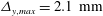 ${\it\Delta}_{y,max}=2.1~\text{mm}$
at the upper slip boundary. The resulting grids contain a total of 12M (sheet-flow) and 16M (vortex ripple) control volumes.
${\it\Delta}_{y,max}=2.1~\text{mm}$
at the upper slip boundary. The resulting grids contain a total of 12M (sheet-flow) and 16M (vortex ripple) control volumes.
After the initial beds were created, the simulation was started from rest, and a time-dependent body force, representing the streamwise oscillatory pressure gradient, was applied to both the fluid and the particles,
 $$\begin{eqnarray}F_{x}(t)={\it\rho}_{f}\frac{\text{d}U(t)}{\text{d}t}.\end{eqnarray}$$
A total of four cycles were simulated for the sheet-flow condition, and nine cycles for the vortex ripple condition. To minimize any morphological change due to startup effects in the vortex ripple case, all particles were held fixed for the first two cycles while the flow developed.
4.2 Characteristic parameters
The transport regime for these two flows can be characterized using two non-dimensional parameters, namely the Shields parameter,
 ${\it\theta}$
, and the suspension number,
${\it\theta}$
, and the suspension number,
 $\mathscr{S}$
. For
$\mathscr{S}$
. For
 ${\it\theta}\gtrsim 0.5$
, bedforms become washed out and the transport occurs in the sheet-flow regime, while the value of
${\it\theta}\gtrsim 0.5$
, bedforms become washed out and the transport occurs in the sheet-flow regime, while the value of
 $\mathscr{S}$
indicates the relative importance of bedload and suspended load to the overall transport. For conditions in the sheet-flow regime, a transition occurs from bedload dominated transport to suspension dominated transport when
$\mathscr{S}$
indicates the relative importance of bedload and suspended load to the overall transport. For conditions in the sheet-flow regime, a transition occurs from bedload dominated transport to suspension dominated transport when
 $\mathscr{S}$
becomes less than approximately 0.8–1.0 (Sumer et al.
Reference Sumer, Kozakiewicz, Fredsøe and Deigaard1996). In oscillatory flows, it is typical to compute the Shields parameter as
$\mathscr{S}$
becomes less than approximately 0.8–1.0 (Sumer et al.
Reference Sumer, Kozakiewicz, Fredsøe and Deigaard1996). In oscillatory flows, it is typical to compute the Shields parameter as
 $$\begin{eqnarray}{\it\theta}=\frac{{\it\sigma}_{max}}{\left({\it\rho}_{p}-{\it\rho}_{f}\right)gd_{50}},\end{eqnarray}$$
where
 ${\it\sigma}_{max}$
is the maximum bed shear stress and can be estimated from the grain roughness friction factor, i.e.
${\it\sigma}_{max}$
is the maximum bed shear stress and can be estimated from the grain roughness friction factor, i.e.
 ${\it\sigma}_{max}=f_{w}U_{max}^{2}/2$
. The corresponding suspension number,
${\it\sigma}_{max}=f_{w}U_{max}^{2}/2$
. The corresponding suspension number,
 $$\begin{eqnarray}\mathscr{S}=\frac{v_{t,50}}{u_{\star }},\end{eqnarray}$$
is the ratio of the particle settling velocity (of the mean size fraction) to the bed friction velocity,
 $u_{\star }=\sqrt{{\it\sigma}_{max}/{\it\rho}_{f}}$
. Using the expression of Swart (Reference Swart1974) for
$u_{\star }=\sqrt{{\it\sigma}_{max}/{\it\rho}_{f}}$
. Using the expression of Swart (Reference Swart1974) for
 $f_{w}$
with a roughness height of
$f_{w}$
with a roughness height of
 $2.5d_{50}$
results in
$2.5d_{50}$
results in
 $[{\it\theta}_{VR},{\it\theta}_{SF}]=\left[0.37,2.24\right]$
and
$[{\it\theta}_{VR},{\it\theta}_{SF}]=\left[0.37,2.24\right]$
and
 $[\mathscr{S}_{VR},\mathscr{S}_{SF}]=[1.12,0.34]$
. The transport is therefore expected to be suspension dominated for the sheet-flow condition, while a suspension number near 1 and relatively large Shields parameter indicate an energetic near-bed flow with significant suspended sediment for the vortex ripple condition.
$[\mathscr{S}_{VR},\mathscr{S}_{SF}]=[1.12,0.34]$
. The transport is therefore expected to be suspension dominated for the sheet-flow condition, while a suspension number near 1 and relatively large Shields parameter indicate an energetic near-bed flow with significant suspended sediment for the vortex ripple condition.

Figure 4. Normalized particle length and time scales for the vortex ripple condition (—) and the sheet-flow condition (○). In (a), the particle scales are normalized by the Kolmogorov scales (top) and the integral scales (bottom). In (b),
 ${\it\tau}_{p}/{\it\tau}_{{\it\Delta}}$
is the ratio of the particle time scale to the time scale of the largest resolved eddy, and
${\it\tau}_{p}/{\it\tau}_{{\it\Delta}}$
is the ratio of the particle time scale to the time scale of the largest resolved eddy, and
 $d_{p}/l_{i}$
is the ratio of the particle size to the eddy size that has the same time scale as the particle, and therefore has a dominant effect on the relative particle velocity.
$d_{p}/l_{i}$
is the ratio of the particle size to the eddy size that has the same time scale as the particle, and therefore has a dominant effect on the relative particle velocity.
To understand the nature of the particle–turbulence interactions, the scaling analysis of Balachandar (Reference Balachandar2009) has been adapted to the present conditions. In figure 4(a), the ranges of the particle length and time scales (
 $d_{p},{\it\tau}_{p}$
) have been made non-dimensional by the approximate Kolmogorov scales (
$d_{p},{\it\tau}_{p}$
) have been made non-dimensional by the approximate Kolmogorov scales (
 ${\it\eta},{\it\tau}_{{\it\eta}}$
) and integral scales (
${\it\eta},{\it\tau}_{{\it\eta}}$
) and integral scales (
 $L,{\it\tau}_{L}$
). Here, the particle time scale is computed as
$L,{\it\tau}_{L}$
). Here, the particle time scale is computed as
 $$\begin{eqnarray}{\it\tau}_{p}=\frac{2{\it\rho}_{p}/{\it\rho}_{f}+1}{36}\frac{d_{p}^{2}}{{\it\nu}^{2}}\frac{1}{C_{d}(Re_{p},0)}.\end{eqnarray}$$
The Kolmogorov scales can be related to the Shields parameter by assuming that
 ${\it\eta}\approx {\it\nu}/u_{\star }$
, where
${\it\eta}\approx {\it\nu}/u_{\star }$
, where
 ${\it\nu}={\it\mu}_{0}/{\it\rho}_{f}$
is the kinematic viscosity, resulting in
${\it\nu}={\it\mu}_{0}/{\it\rho}_{f}$
is the kinematic viscosity, resulting in
 $$\begin{eqnarray}{\it\eta}=\frac{{\it\nu}}{\sqrt{{\it\theta}\left({\displaystyle \frac{{\it\rho}_{p}}{{\it\rho}_{f}}}-1\right)gd_{50}}},\quad {\it\tau}_{{\it\eta}}=\frac{{\it\nu}}{{\it\theta}\left({\displaystyle \frac{{\it\rho}_{p}}{{\it\rho}_{f}}}-1\right)gd_{50}}.\end{eqnarray}$$
The integral time scale is estimated as
 ${\it\tau}_{L}=L/U_{rms}$
, where the integral length scale,
${\it\tau}_{L}=L/U_{rms}$
, where the integral length scale,
 $L$
, is taken to be either the ripple height,
$L$
, is taken to be either the ripple height,
 $h_{r}=0.076~\text{m}$
, or the maximum sheet-flow boundary layer thickness,
$h_{r}=0.076~\text{m}$
, or the maximum sheet-flow boundary layer thickness,
 $H_{bl}\approx 0.02~\text{m}$
(cf. figure 7). From figure 4(a), it can be seen that
$H_{bl}\approx 0.02~\text{m}$
(cf. figure 7). From figure 4(a), it can be seen that
 ${\it\eta}\ll d_{p}\ll L$
and also that
${\it\eta}\ll d_{p}\ll L$
and also that
 ${\it\tau}_{{\it\eta}}\ll {\it\tau}_{p}\ll {\it\tau}_{L}$
for the range of particle sizes used in both conditions. The particles are between 10 and 50 times larger than
${\it\tau}_{{\it\eta}}\ll {\it\tau}_{p}\ll {\it\tau}_{L}$
for the range of particle sizes used in both conditions. The particles are between 10 and 50 times larger than
 ${\it\eta}$
, with corresponding Stokes numbers in the range
${\it\eta}$
, with corresponding Stokes numbers in the range
 $9\lesssim St\lesssim 34$
.
$9\lesssim St\lesssim 34$
.
The relative velocity of the particles and the resulting momentum exchange between phases are therefore controlled primarily by an intermediate-size eddy in the inertial range, which has the same time scale as the
 $d_{p}$
size particle, in addition to the gravitational settling. The size of this eddy is
$d_{p}$
size particle, in addition to the gravitational settling. The size of this eddy is
 $l_{i}={\it\tau}_{p}^{3/2}{\it\epsilon}^{1/2}$
, where
$l_{i}={\it\tau}_{p}^{3/2}{\it\epsilon}^{1/2}$
, where
 ${\it\epsilon}\approx {\it\nu}^{3}/{\it\eta}^{4}$
is the energy dissipation rate. When adopting a point-particle LES approach, it is important to capture the effect of the
${\it\epsilon}\approx {\it\nu}^{3}/{\it\eta}^{4}$
is the energy dissipation rate. When adopting a point-particle LES approach, it is important to capture the effect of the
 $l_{i}$
sized eddies on the particles, meaning that their time scale should be larger than the time scale of the largest resolved eddy,
$l_{i}$
sized eddies on the particles, meaning that their time scale should be larger than the time scale of the largest resolved eddy,
 ${\it\tau}_{{\it\Delta}}={\it\tau}_{{\it\eta}}({\it\Delta}/{\it\eta})^{2/3}$
(Balachandar Reference Balachandar2009). In figure 4(b), the ratio
${\it\tau}_{{\it\Delta}}={\it\tau}_{{\it\eta}}({\it\Delta}/{\it\eta})^{2/3}$
(Balachandar Reference Balachandar2009). In figure 4(b), the ratio
 ${\it\tau}_{p}/{\it\tau}_{{\it\Delta}}$
is plotted versus the range of the non-dimensional particle size,
${\it\tau}_{p}/{\it\tau}_{{\it\Delta}}$
is plotted versus the range of the non-dimensional particle size,
 $d_{p}/l_{i}$
. For the present conditions, the
$d_{p}/l_{i}$
. For the present conditions, the
 $l_{i}$
size eddies are between approximately 2.5 and 5 times larger than the particles, and these eddies are resolved by the computational grids (
$l_{i}$
size eddies are between approximately 2.5 and 5 times larger than the particles, and these eddies are resolved by the computational grids (
 ${\it\tau}_{p}/{\it\tau}_{{\it\Delta}}\gtrsim 1$
). However, we note that especially for the smallest particle fractions the
${\it\tau}_{p}/{\it\tau}_{{\it\Delta}}\gtrsim 1$
). However, we note that especially for the smallest particle fractions the
 $l_{i}$
scale eddies may not be resolved by more than approximately two grid points, and the contribution of subgrid-scale eddies to the particle relative velocity may not be negligible. Our future efforts will involve incorporation of a stochastic model (i.e. Pozorski & Apte Reference Pozorski and Apte2009) to account for and investigate these effects.
$l_{i}$
scale eddies may not be resolved by more than approximately two grid points, and the contribution of subgrid-scale eddies to the particle relative velocity may not be negligible. Our future efforts will involve incorporation of a stochastic model (i.e. Pozorski & Apte Reference Pozorski and Apte2009) to account for and investigate these effects.
The ratio
 $g/a_{k}$
, where
$g/a_{k}$
, where
 $a_{k}={\it\epsilon}^{2/3}/{\it\eta}^{1/3}$
is the Kolmogorov acceleration, is much less than 1 for the present conditions, indicating that turbulence influences the relative particle velocity much more than gravitational settling for the present conditions. The particle Reynolds numbers can then be estimated from the expression provided by Balachandar (Reference Balachandar2009),
$a_{k}={\it\epsilon}^{2/3}/{\it\eta}^{1/3}$
is the Kolmogorov acceleration, is much less than 1 for the present conditions, indicating that turbulence influences the relative particle velocity much more than gravitational settling for the present conditions. The particle Reynolds numbers can then be estimated from the expression provided by Balachandar (Reference Balachandar2009),
 $$\begin{eqnarray}Re_{p}=\sqrt{\frac{1}{2{\it\rho}_{p}/{\it\rho}_{f}+1}}\frac{{\it\rho}_{p}/{\it\rho}_{f}-1}{3\sqrt{C_{d}(Re_{p},0)}}\left(\frac{d_{p}}{{\it\eta}}\right)^{2},\end{eqnarray}$$
which results in
 $17\leqslant Re_{p}\leqslant 124$
for the vortex ripple condition and
$17\leqslant Re_{p}\leqslant 124$
for the vortex ripple condition and
 $25\leqslant Re_{p}\leqslant 175$
for the sheet-flow condition.
$25\leqslant Re_{p}\leqslant 175$
for the sheet-flow condition.
4.3 Experimental validation
To compare with the phase resolved experimental measurements, the simulation results have been averaged over the homogeneous directions (
 $X$
and
$X$
and
 $Z$
for the sheet-flow condition,
$Z$
for the sheet-flow condition,
 $Z$
for the vortex ripple condition) and have been ensemble averaged over the final three cycles of each simulation.
$Z$
for the vortex ripple condition) and have been ensemble averaged over the final three cycles of each simulation.
4.3.1 Near-bed velocities
Figure 5 shows the spanwise and ensemble averaged near-ripple fluid velocity vector fields at eight phases of the flow for the vortex ripple condition. The major features of the flow are consistent with the particle image velocimetry (PIV) results reported by Van der Werf et al. (Reference Van der Werf, Doucette, O’Donoghue and Ribberink2007) (not shown), which will briefly be summarized here. At the moments of flow reversal (a,e), a large vortex is ejected from the ripple trough. The vortex ejected over the lee slope at onshore reversal (e) is significantly stronger than the one ejected over the stoss slope during offshore reversal (a). This, combined with strong erosion of the ripple crest during the onshore half-cycle (b,c,d), contributes to the asymmetric shape and onshore migration of the ripples. The overshoot of the near-bed flow velocity can be seen clearly during the acceleration and deceleration phases (b and f) above the ripple crest.

Figure 5. Spanwise and ensemble averaged 2D vector fields shown at selected phases for the vortex ripple case.
A direct comparison with near-ripple experimental measurements (PIV) is made in figure 6 for eight points along the ripple. The data were extracted from a region
 $9~\text{mm}$
above the simulated ripple surface (determined as the surface where
$9~\text{mm}$
above the simulated ripple surface (determined as the surface where
 ${\it\Theta}_{p}=0.6$
), corresponding as closely as possible to the experiments. Overall, quite good agreement is achieved at most positions along the ripple. The maximum on- and offshore velocities are very well predicted by the model, both above the crest and in the trough, indicating that vortex creation and ejection is well captured. The main disagreement can be found over the lee slope, shown in (a,c), during the creation of the stoss side vortex (
${\it\Theta}_{p}=0.6$
), corresponding as closely as possible to the experiments. Overall, quite good agreement is achieved at most positions along the ripple. The maximum on- and offshore velocities are very well predicted by the model, both above the crest and in the trough, indicating that vortex creation and ejection is well captured. The main disagreement can be found over the lee slope, shown in (a,c), during the creation of the stoss side vortex (
 $0.6\lesssim t/T\lesssim 0.9$
), which is possibly due to slight differences in the simulated and experimental ripple profiles. Some of the higher-frequency variation observed in the simulation results, but not the experimental measurements, could be due to the periodic simulation domain. Periodicity in the streamwise and spanwise directions is likely to promote a more identical cycle-to-cycle flow than in the laboratory, and this will preserve the signature of smaller-time-scale motions in the mean flow. Extending the ensemble average to the last five cycles (to match with the experiments) did not change the character of this result.
$0.6\lesssim t/T\lesssim 0.9$
), which is possibly due to slight differences in the simulated and experimental ripple profiles. Some of the higher-frequency variation observed in the simulation results, but not the experimental measurements, could be due to the periodic simulation domain. Periodicity in the streamwise and spanwise directions is likely to promote a more identical cycle-to-cycle flow than in the laboratory, and this will preserve the signature of smaller-time-scale motions in the mean flow. Extending the ensemble average to the last five cycles (to match with the experiments) did not change the character of this result.

Figure 6. Comparison of predicted and measured velocities for the vortex ripple condition: —, simulation; ○, experiment (PIV); - - -, free-stream velocity;
 $x/{\it\lambda}=-0.09$
(a), 0.04 (b),
$x/{\it\lambda}=-0.09$
(a), 0.04 (b),
 $-0.22$
(c), 0.16 (d),
$-0.22$
(c), 0.16 (d),
 $-0.35$
(e), 0.29 (f),
$-0.35$
(e), 0.29 (f),
 $-0.48$
(g), 0.42 (h).
$-0.48$
(g), 0.42 (h).
Figure 7 compares the measured and predicted velocity profiles at several phases for the sheet-flow condition. The simulations capture the velocity skewness of the boundary layer, and the agreement with the experimental measurements is quite good for all phases with the exception of the onshore acceleration (
 $t/T=0.12$
) phase, which lags behind the measured profile. It is worth noting that due to three-dimensional effects in the flow tunnel, the measured free-stream velocities are somewhat lower than the piston velocity used to drive the flow, and therefore exact hydrodynamic equivalence with the experiments is not achieved by forcing the flow using (4.1). However, the computed flow velocity profile follows the measured data very well from the fully packed bed up to the top of the suspension layer (
$t/T=0.12$
) phase, which lags behind the measured profile. It is worth noting that due to three-dimensional effects in the flow tunnel, the measured free-stream velocities are somewhat lower than the piston velocity used to drive the flow, and therefore exact hydrodynamic equivalence with the experiments is not achieved by forcing the flow using (4.1). However, the computed flow velocity profile follows the measured data very well from the fully packed bed up to the top of the suspension layer (
 $Y\approx 40~\text{mm}$
), which indicates the good performance of the model across regions with a wide range of sediment concentrations.
$Y\approx 40~\text{mm}$
), which indicates the good performance of the model across regions with a wide range of sediment concentrations.

Figure 7. Comparison of predicted and measured velocities for the sheet-flow condition: —, simulation; ○, experiment.

Figure 8. Suspended sediment concentrations for the vortex ripple condition. The figure on the left-hand side shows the time and ripple averaged suspended sediment concentration as a function of height: —, simulation; ○, experiment (acoustic); ▾, experiment (optical); - - -, a fit to (4.9). The contour plots on the right-hand side show the ensemble averaged suspended sediment concentration at select phases (
 $\log _{10}$
scale).
$\log _{10}$
scale).
4.3.2 Suspended sediment concentrations
The time and ripple-length (
 $X$
) averaged suspended sediment concentrations predicted by the model are compared with the measurements on the left-hand side of figure 8 for the vortex ripple condition. The simulated concentration results generally lie between the acoustic and the optical measurements and illustrate the well-known negative exponential decay above the ripple crest (Bosman & Steetzel Reference Bosman and Steetzel1986; Nielsen Reference Nielsen1992; Ribberink & Al-Salem Reference Ribberink and Al-Salem1994), of the form
$X$
) averaged suspended sediment concentrations predicted by the model are compared with the measurements on the left-hand side of figure 8 for the vortex ripple condition. The simulated concentration results generally lie between the acoustic and the optical measurements and illustrate the well-known negative exponential decay above the ripple crest (Bosman & Steetzel Reference Bosman and Steetzel1986; Nielsen Reference Nielsen1992; Ribberink & Al-Salem Reference Ribberink and Al-Salem1994), of the form
 $$\begin{eqnarray}C(z)=C_{0}\exp \left(\frac{-Yv_{t,50}}{{\it\epsilon}_{s}}\right).\end{eqnarray}$$
Here,
 $C_{0}$
is the concentration just above the ripple crest and
$C_{0}$
is the concentration just above the ripple crest and
 ${\it\epsilon}_{s}$
is the sediment diffusivity. A fit to (4.9) with
${\it\epsilon}_{s}$
is the sediment diffusivity. A fit to (4.9) with
 $C_{0}=2.37~\text{g}~\text{l}^{-1}$
and
$C_{0}=2.37~\text{g}~\text{l}^{-1}$
and
 ${\it\epsilon}_{s}=0.0034~\text{m}^{2}~\text{s}^{-1}$
provides a good match to the data and is shown as a dashed line in figure 8. This suggests a vertical length scale of suspended sediment mixing of
${\it\epsilon}_{s}=0.0034~\text{m}^{2}~\text{s}^{-1}$
provides a good match to the data and is shown as a dashed line in figure 8. This suggests a vertical length scale of suspended sediment mixing of
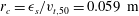 $r_{c}={\it\epsilon}_{s}/v_{t,50}=0.059~\text{m}$
, or approximately
$r_{c}={\it\epsilon}_{s}/v_{t,50}=0.059~\text{m}$
, or approximately
 $0.8h_{r}$
, which agrees well with the data of Ribberink & Al-Salem (Reference Ribberink and Al-Salem1994). Van der Werf et al. (Reference Van der Werf, Magar, Malarkey, Guizien and ODonoghue2008) and Malarkey et al. (Reference Malarkey, Magar and Davies2015) show a similar comparison based on two-dimensional advection–diffusion based models. The much larger discrepancies in their results were attributed to an inadequate representation of turbulent sediment diffusion. A strength of the present model is that the time-dependent concentration field depends only on Lagrangian particle motion, with no uncertainties introduced to the concentration field through an advection–diffusion solution, reference concentration or pickup function. The results also suggest that in addition to the turbulence, particle-size effects may also play an important role in determining the cycle averaged concentration, as examined in the following section.
$0.8h_{r}$
, which agrees well with the data of Ribberink & Al-Salem (Reference Ribberink and Al-Salem1994). Van der Werf et al. (Reference Van der Werf, Magar, Malarkey, Guizien and ODonoghue2008) and Malarkey et al. (Reference Malarkey, Magar and Davies2015) show a similar comparison based on two-dimensional advection–diffusion based models. The much larger discrepancies in their results were attributed to an inadequate representation of turbulent sediment diffusion. A strength of the present model is that the time-dependent concentration field depends only on Lagrangian particle motion, with no uncertainties introduced to the concentration field through an advection–diffusion solution, reference concentration or pickup function. The results also suggest that in addition to the turbulence, particle-size effects may also play an important role in determining the cycle averaged concentration, as examined in the following section.
In figure 8(a–h), the spanwise and ensemble averaged suspended sediment concentration fields are shown at several phases of the cycle: at off–onshore flow reversal (a), a suspended sediment cloud with moderate concentrations can be seen over the stoss side slope, while a smaller region of high concentration is seen in the trough. This sediment is carried over one or two ripple lengths as the flow accelerates onshore, with a certain amount of sediment settling back to the bed during this time (b,c). At the same time, the ripple crest is eroded by the strong onshore flow (b,c,d). As the flow begins to decelerate (d), there is abundant sediment in suspension along the lee side slope due to the lee vortex generation. The lee vortex is therefore very rich in suspended sediment when it is ejected around the time of on–offshore flow reversal, resulting in a large suspended sediment cloud over the ripple crest (e,f). This cloud passes through the periodic domain and over the crest three times at roughly
 $t/T=0.5$
,
$t/T=0.5$
,
 $t/T=0.7$
and
$t/T=0.7$
and
 $t/T=0.9$
, consistent with experimental observations.
$t/T=0.9$
, consistent with experimental observations.

Figure 9. Sediment concentrations for the sheet-flow case. On the left-hand side, concentrations are shown at select phases in the sheet-flow layer: —, simulation; ○, experiment (CCM);
 $t/T=0$
(a), 0.12 (b), 0.22 (c), 0.34 (d), 0.44 (e), 0.54 (f), 0.74 (g), 0.92 (h). On the right-hand side, the period averaged concentration is shown with additional suction system measurements (▴) and the fit to (4.10) for
$t/T=0$
(a), 0.12 (b), 0.22 (c), 0.34 (d), 0.44 (e), 0.54 (f), 0.74 (g), 0.92 (h). On the right-hand side, the period averaged concentration is shown with additional suction system measurements (▴) and the fit to (4.10) for
 $Y>1~\text{cm}$
(- - -) with
$Y>1~\text{cm}$
(- - -) with
 ${\it\alpha}=2.1$
.
${\it\alpha}=2.1$
.
The concentration profiles in the lower sheet-flow layer are shown in figure 9 for the sheet-flow condition, and are compared with experimental measurements made using a conductivity concentration meter (CCM). The concentration measurements have been normalized by the undisturbed bed concentration (
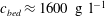 $c_{bed}\approx 1600~\text{g}~\text{l}^{-1}$
). The computed sediment concentration follows the CCM measurements very well in both the pickup layer (
$c_{bed}\approx 1600~\text{g}~\text{l}^{-1}$
). The computed sediment concentration follows the CCM measurements very well in both the pickup layer (
 $Y<-2~\text{mm}$
) and the upper sheet-flow layer (
$Y<-2~\text{mm}$
) and the upper sheet-flow layer (
 $-2~\text{mm}<Y<2~\text{mm}$
). The main discrepancy seems to be around the initial deceleration towards on–offshore flow reversal (c,d), which suggests that the model underpredicts the pickup of sediment from the lower part of the bed at the maximum flow. It is possible that the effects of unresolved subgrid-scale fluid–particle interactions are important during this phase of high shear stress, which warrants future investigation of stochastic models for particle–fluid interaction under such conditions. The overall agreement, however, is considered to be good, which indicates the strength of the model in simulating particle–particle and fluid–particle interactions in such high-concentration regions.
$-2~\text{mm}<Y<2~\text{mm}$
). The main discrepancy seems to be around the initial deceleration towards on–offshore flow reversal (c,d), which suggests that the model underpredicts the pickup of sediment from the lower part of the bed at the maximum flow. It is possible that the effects of unresolved subgrid-scale fluid–particle interactions are important during this phase of high shear stress, which warrants future investigation of stochastic models for particle–fluid interaction under such conditions. The overall agreement, however, is considered to be good, which indicates the strength of the model in simulating particle–particle and fluid–particle interactions in such high-concentration regions.
In the plot on the right-hand side of figure 9, the period averaged concentration profile is compared with measurements made using a CCM and a suction sampling device by O’Donoghue & Wright (Reference O’Donoghue and Wright2004b ) over a larger range. The simulation is in reasonable agreement with the lower suction measurements and the upper CCM measurements. Also shown is the fit to the power law equation proposed by Ribberink & Al-Salem (Reference Ribberink and Al-Salem1994),
 $$\begin{eqnarray}C(z)=C_{0}\left(\frac{Y_{ref}}{Y}\right)^{{\it\alpha}},\end{eqnarray}$$
where
 $C_{0}$
is taken to be the reference concentration at 1 cm above the undisturbed bed level, and the exponent
$C_{0}$
is taken to be the reference concentration at 1 cm above the undisturbed bed level, and the exponent
 ${\it\alpha}\approx 2.1$
provided a good fit to their data for slightly finer sand than considered here (
${\it\alpha}\approx 2.1$
provided a good fit to their data for slightly finer sand than considered here (
 $d_{50}=0.21~\text{mm}$
). In the simulation, less sediment is retained in suspension for
$d_{50}=0.21~\text{mm}$
). In the simulation, less sediment is retained in suspension for
 $Y>1~\text{cm}$
than was measured by the suction system, and a stronger decay is observed, with
$Y>1~\text{cm}$
than was measured by the suction system, and a stronger decay is observed, with
 ${\it\alpha}\approx 3.3$
.
${\it\alpha}\approx 3.3$
.
4.3.3 Net sediment transport
In the experiments, the net sediment transport rate was estimated by accounting for bed profile changes as well as the amounts of the sediment collected in traps at both ends of the tunnel. For the vortex ripple condition, Van der Werf et al. (Reference Van der Werf, Doucette, O’Donoghue and Ribberink2007) found a small offshore directed net transport,
 $q_{vr}=-3.69\times 10^{-6}~\text{m}^{2}~\text{s}^{-1}$
, while the ripples were observed to migrate onshore with a velocity of
$q_{vr}=-3.69\times 10^{-6}~\text{m}^{2}~\text{s}^{-1}$
, while the ripples were observed to migrate onshore with a velocity of
 $u_{mig}\approx 18~\text{mm}~\text{s}^{-1}$
. The simulated ripple migration speed,
$u_{mig}\approx 18~\text{mm}~\text{s}^{-1}$
. The simulated ripple migration speed,
 $u_{mig}\approx 14~\text{mm}~\text{s}^{-1}$
, is in very good agreement. However, the net sediment transport rate in the simulations is found to be onshore directed, with a magnitude of
$u_{mig}\approx 14~\text{mm}~\text{s}^{-1}$
, is in very good agreement. However, the net sediment transport rate in the simulations is found to be onshore directed, with a magnitude of
 $q_{vr}=8.70\times 10^{-6}~\text{m}^{2}~\text{s}^{-1}$
, suggesting that some of the offshore directed suspended sediment fluxes are underpredicted by the model. For the sheet-flow condition, O’Donoghue & Wright (Reference O’Donoghue and Wright2004b
) reported
$q_{vr}=8.70\times 10^{-6}~\text{m}^{2}~\text{s}^{-1}$
, suggesting that some of the offshore directed suspended sediment fluxes are underpredicted by the model. For the sheet-flow condition, O’Donoghue & Wright (Reference O’Donoghue and Wright2004b
) reported
 $q_{sf}=53\times 10^{-6}~\text{m}^{2}~\text{s}^{-1}$
, which is in reasonable agreement with the simulated value of
$q_{sf}=53\times 10^{-6}~\text{m}^{2}~\text{s}^{-1}$
, which is in reasonable agreement with the simulated value of
 $q_{sf}=42.3\times 10^{-6}~\text{m}^{2}~\text{s}^{-1}$
. Ribberink & Al-Salem (Reference Ribberink and Al-Salem1994) found a strong correlation between the net transport and the third velocity moment for both rippled bed and sheet-flow conditions,
$q_{sf}=42.3\times 10^{-6}~\text{m}^{2}~\text{s}^{-1}$
. Ribberink & Al-Salem (Reference Ribberink and Al-Salem1994) found a strong correlation between the net transport and the third velocity moment for both rippled bed and sheet-flow conditions,
 $q=A\langle U^{3}\rangle$
. Using
$q=A\langle U^{3}\rangle$
. Using
 $A=150\times 10^{-6}$
, which corresponds to their flows with similar periods to the ones considered here, gives
$A=150\times 10^{-6}$
, which corresponds to their flows with similar periods to the ones considered here, gives
 $q_{vr}=3.12$
and
$q_{vr}=3.12$
and
 $q_{sf}=49.4$
, quite close to and in the same direction as both simulation results.
$q_{sf}=49.4$
, quite close to and in the same direction as both simulation results.
4.4 Three-dimensional description
Up to this point, streamwise and spanwise averaging have been used to reduce these flows to either one or two spatial dimensions (in addition to time). However, at the Reynolds numbers involved in the experiments, the turbulent structure of the flow and its interaction with the sediment are known to be highly three-dimensional (Ozdemir et al.
Reference Ozdemir, Hsu and Balachandar2010; Penko et al.
Reference Penko, Calantoni, Rodriguez-Abudo, Foster and Slinn2013). Of particular importance are the three-dimensional vortical structures which provide the regions of upward directed flow necessary for sediment to travel away from the bed and remain in suspension. The swirling strength criterion (
 ${\it\lambda}_{ci}$
) of Zhou et al. (Reference Zhou, Adrian, Balachandar and Kendall1999a
) is used to extract these features and examine their interaction with the particle phase by plotting isosurfaces of
${\it\lambda}_{ci}$
) of Zhou et al. (Reference Zhou, Adrian, Balachandar and Kendall1999a
) is used to extract these features and examine their interaction with the particle phase by plotting isosurfaces of
 ${\it\lambda}_{ci}$
along with instantaneous particle positions in figures 10 and 11. To remove very-small-scale features from the visualizations, a low-pass filter has been applied to the instantaneous velocity fields before computing
${\it\lambda}_{ci}$
along with instantaneous particle positions in figures 10 and 11. To remove very-small-scale features from the visualizations, a low-pass filter has been applied to the instantaneous velocity fields before computing
 $\boldsymbol{{\rm\nabla}}\boldsymbol{u}_{f}$
and its eigenvalues. To allow spatio-temporal size sorting to be identified, individual particles have been coloured and rendered according to their size.
$\boldsymbol{{\rm\nabla}}\boldsymbol{u}_{f}$
and its eigenvalues. To allow spatio-temporal size sorting to be identified, individual particles have been coloured and rendered according to their size.

Figure 10. Three-dimensional snapshots of vortex cores visualized as isosurfaces of
 ${\it\lambda}_{ci}=20~\text{s}^{-1}$
and particle positions at eight phases of the oscillatory flow for the vortex ripple condition. Individual particles have been rendered at twice their actual size to aid in visualization;
${\it\lambda}_{ci}=20~\text{s}^{-1}$
and particle positions at eight phases of the oscillatory flow for the vortex ripple condition. Individual particles have been rendered at twice their actual size to aid in visualization;
 $t/T=0$
(a), 0.12 (b), 0.22 (c), 0.34 (d), 0.44 (e), 0.54 (f), 0.74 (g), 0.92 (h).
$t/T=0$
(a), 0.12 (b), 0.22 (c), 0.34 (d), 0.44 (e), 0.54 (f), 0.74 (g), 0.92 (h).

Figure 11. As in figure 10, but for the sheet-flow condition, with an isovalue of
 ${\it\lambda}_{ci}=70~\text{s}^{-1}$
. Particles are rendered at their actual size;
${\it\lambda}_{ci}=70~\text{s}^{-1}$
. Particles are rendered at their actual size;
 $t/T=0$
(a), 0.12 (b), 0.22 (c), 0.34 (d), 0.44 (e), 0.54 (f), 0.74 (g), 0.92 (h).
$t/T=0$
(a), 0.12 (b), 0.22 (c), 0.34 (d), 0.44 (e), 0.54 (f), 0.74 (g), 0.92 (h).
Figure 10 shows these results for the vortex ripple condition at eight phases of the wave cycle as in the previous section. The largest vortex cores can be seen to be pseudo-two-dimensional, spanning the entire width of the domain in the
 $Z$
direction. However, significant three-dimensional small-scale structures are also evident throughout the cycle in the form of entangled vortex filaments around the larger two-dimensional vortex cores and streaks along the bed surface, similar to observations from other numerical studies (e.g. Vittori & Verzicco Reference Vittori and Verzicco1998; Scandura, Vittori & Blondeaux Reference Scandura, Vittori and Blondeaux2000; Zedler & Street Reference Zedler and Street2006; Schmeeckle Reference Schmeeckle2014). These coherent vortical features have a clear influence on particle motion throughout the cycle: at off–onshore flow reversal (figure 10
a), a small vortex is detected at the bottom of the stoss slope in an area of high suspended sediment concentration (see also figure 8
a), also observed by Van der Werf et al. (Reference Van der Werf, Doucette, O’Donoghue and Ribberink2007). At the same time, remnants of several vortices ejected from the ripple trough during previous cycles can be seen higher in the water column, maintaining large numbers of particles around them. As the flow speed increases in the onshore direction (b), near-bed vortical streaks appear around the crest, and as the flow separates over the lee slope, a number of particles are picked up by these near-bed features. As the flow speed peaks (c), the 3D streaks cover the entire surface of the ripple, and some have rolled up into larger pseudo-two-dimensional vortex cores. Once the flow starts to reduce speed and reverse direction (d,e), these streaks are lifted from the bed and in the trough they roll up around a large two-dimensional vortex core, lifting a substantial number of particles from the bed. This particle cloud extends as high as
$Z$
direction. However, significant three-dimensional small-scale structures are also evident throughout the cycle in the form of entangled vortex filaments around the larger two-dimensional vortex cores and streaks along the bed surface, similar to observations from other numerical studies (e.g. Vittori & Verzicco Reference Vittori and Verzicco1998; Scandura, Vittori & Blondeaux Reference Scandura, Vittori and Blondeaux2000; Zedler & Street Reference Zedler and Street2006; Schmeeckle Reference Schmeeckle2014). These coherent vortical features have a clear influence on particle motion throughout the cycle: at off–onshore flow reversal (figure 10
a), a small vortex is detected at the bottom of the stoss slope in an area of high suspended sediment concentration (see also figure 8
a), also observed by Van der Werf et al. (Reference Van der Werf, Doucette, O’Donoghue and Ribberink2007). At the same time, remnants of several vortices ejected from the ripple trough during previous cycles can be seen higher in the water column, maintaining large numbers of particles around them. As the flow speed increases in the onshore direction (b), near-bed vortical streaks appear around the crest, and as the flow separates over the lee slope, a number of particles are picked up by these near-bed features. As the flow speed peaks (c), the 3D streaks cover the entire surface of the ripple, and some have rolled up into larger pseudo-two-dimensional vortex cores. Once the flow starts to reduce speed and reverse direction (d,e), these streaks are lifted from the bed and in the trough they roll up around a large two-dimensional vortex core, lifting a substantial number of particles from the bed. This particle cloud extends as high as
 $100~\text{mm}$
above crest level as the lee vortex is ejected during flow reversal (e) and the flow accelerates offshore (f). During the offshore half-cycle (e–h), a similar process takes place, but the near-bed streaks have a longer time to develop and become more elongated along the ripple surface (g,h) due to the asymmetry of the wave.
$100~\text{mm}$
above crest level as the lee vortex is ejected during flow reversal (e) and the flow accelerates offshore (f). During the offshore half-cycle (e–h), a similar process takes place, but the near-bed streaks have a longer time to develop and become more elongated along the ripple surface (g,h) due to the asymmetry of the wave.
Comparatively, the same results for the sheet-flow condition, shown in figure 11, exhibit a lack of large-scale vortex shedding, and more uniform near-bed streaks that are significantly stronger (note that the magnitude of the
 ${\it\lambda}_{ci}$
isosurfaces is 3.5 times larger than in figure 10). Similarly to the vortex ripple condition, the flow is almost clear of vortical structures at the beginning of the cycle, apart from remnants of broken vortex cores from the last wave cycle. During the onshore flow acceleration (figure 11
b,c), densely located energetic vortical structures are generated close to the bed surface. These streaks remain close to the bed until maximum onshore flow (c), and as the flow decelerates (d), they are lifted 10–20 mm above the initial bed level, carrying large quantities of particles with them. At on–offshore flow reversal (e), most of the near-bed streaks have been dissipated, although many of them remain higher in the water column. During the subsequent offshore half-cycle (f–h), a similar process follows and, similarly to the vortex ripple condition, the near-bed streaks become better developed and elongated due to the asymmetry of the mean flow.
${\it\lambda}_{ci}$
isosurfaces is 3.5 times larger than in figure 10). Similarly to the vortex ripple condition, the flow is almost clear of vortical structures at the beginning of the cycle, apart from remnants of broken vortex cores from the last wave cycle. During the onshore flow acceleration (figure 11
b,c), densely located energetic vortical structures are generated close to the bed surface. These streaks remain close to the bed until maximum onshore flow (c), and as the flow decelerates (d), they are lifted 10–20 mm above the initial bed level, carrying large quantities of particles with them. At on–offshore flow reversal (e), most of the near-bed streaks have been dissipated, although many of them remain higher in the water column. During the subsequent offshore half-cycle (f–h), a similar process follows and, similarly to the vortex ripple condition, the near-bed streaks become better developed and elongated due to the asymmetry of the mean flow.
4.5 Behaviour of different size fractions
By rendering the particles according to size in figures 10 and 11, strong spatio-temporal particle-size sorting patterns are revealed, both near the bed and in suspension, which appear to be strongly influenced by the three-dimensional flow field.
4.5.1 Near the bed
Throughout most of the wave cycle in the vortex ripple condition, the bed surface is covered by large particles, and a similarly coarse surface layer can be seen in the low-velocity phases under sheet-flow conditions. The composition of this near-bed surface layer is important, as it directly influences which particles are brought into suspension and at what phase of the cycle, thus influencing the net transport behaviour (Dohmen-Janssen et al.
Reference Dohmen-Janssen, Kroekenstoel, Hassan and Ribberink2002). This feature is explored in figure 12, where the relative abundance of different particle sizes in the near-bed layer,
 $Y^{\prime }=Y_{bed}+2.5d_{50}$
, has been plotted versus phase. To extract this result from the particle data, the instantaneous bed level,
$Y^{\prime }=Y_{bed}+2.5d_{50}$
, has been plotted versus phase. To extract this result from the particle data, the instantaneous bed level,
 $Y_{bed}(x,z)$
, is taken to be the local elevation where
$Y_{bed}(x,z)$
, is taken to be the local elevation where
 ${\it\Theta}_{p}=0.6$
, and particles are binned into five fractions with mean diameters
${\it\Theta}_{p}=0.6$
, and particles are binned into five fractions with mean diameters
 $d_{10}$
,
$d_{10}$
,
 $d_{30}$
,
$d_{30}$
,
 $d_{50}$
,
$d_{50}$
,
 $d_{70}$
and
$d_{70}$
and
 $d_{90}$
. In a perfectly mixed condition, each of these fractions would be expected to contribute 20 % to the total composition. The departure of the results in figure 12 from this behaviour demonstrates the effectiveness of different flow-driven particle-size sorting mechanisms.
$d_{90}$
. In a perfectly mixed condition, each of these fractions would be expected to contribute 20 % to the total composition. The departure of the results in figure 12 from this behaviour demonstrates the effectiveness of different flow-driven particle-size sorting mechanisms.

Figure 12. Relative abundance of different particle-size fractions in the near-bed layer,
 $Y^{\prime }=Y_{bed}+2.5d_{50}$
: (-
$Y^{\prime }=Y_{bed}+2.5d_{50}$
: (-
 $\cdot$
-)
$\cdot$
-)
 $d_{10}$
, (- - -)
$d_{10}$
, (- - -)
 $d_{30}$
, (—)
$d_{30}$
, (—)
 $d_{50}$
, (—▴—)
$d_{50}$
, (—▴—)
 $d_{70}$
, (—▪—)
$d_{70}$
, (—▪—)
 $d_{90}$
; vortex ripple (a,c), sheet flow (b,d).
$d_{90}$
; vortex ripple (a,c), sheet flow (b,d).
Under vortex ripple conditions, the composition of the near-bed layer is nearly constant for the low-velocity offshore half-cycle, and is disproportionately coarse with roughly 2/3 of the solid volume being coarser than
 $d_{60}$
. During onshore acceleration, when the near-bed vortical streaks touch the bed surface (figure 10
b,c), high-speed flow near the bed is able to lift the coarse fractions into suspension. This exposes the finer fractions below, especially along the stoss side of the ripple, which experiences some of the largest near-bed velocities (see figure 6). Consequently, the particle sizes in the near-bed layer are better mixed during the onshore half-cycle and during formation of the lee vortex. When the lee vortex is ejected and passes over the crest (figure 10
f,g), the largest fractions quickly settle down, coarsening the surface layer. Being exposed to the high velocities and vortical streaks for most of the cycle, the crest tends to lose coarse particles, while the trough area is less affected by the streaks and hence accumulates the coarse fractions. Such a sorting process agrees with time averaged measurements of the settling velocity distribution (see Van der Werf et al. (Reference Van der Werf, Magar, Malarkey, Guizien and ODonoghue2008) figure 4). The near-constant composition in the near-bed layer reflects the fact that mixing and particle-size sorting largely occur in the suspension under vortex ripple conditions, driven by large-scale vortex shedding.
$d_{60}$
. During onshore acceleration, when the near-bed vortical streaks touch the bed surface (figure 10
b,c), high-speed flow near the bed is able to lift the coarse fractions into suspension. This exposes the finer fractions below, especially along the stoss side of the ripple, which experiences some of the largest near-bed velocities (see figure 6). Consequently, the particle sizes in the near-bed layer are better mixed during the onshore half-cycle and during formation of the lee vortex. When the lee vortex is ejected and passes over the crest (figure 10
f,g), the largest fractions quickly settle down, coarsening the surface layer. Being exposed to the high velocities and vortical streaks for most of the cycle, the crest tends to lose coarse particles, while the trough area is less affected by the streaks and hence accumulates the coarse fractions. Such a sorting process agrees with time averaged measurements of the settling velocity distribution (see Van der Werf et al. (Reference Van der Werf, Magar, Malarkey, Guizien and ODonoghue2008) figure 4). The near-constant composition in the near-bed layer reflects the fact that mixing and particle-size sorting largely occur in the suspension under vortex ripple conditions, driven by large-scale vortex shedding.
Under sheet-flow conditions, the overall composition of the near-bed layer is much more dynamic. A strong coarse-over-fine layering of particles is seen in low-velocity phases (figure 11 a,e), which results in a very coarse near-bed composition. As the flow accelerates onshore, these coarse particles are lifted to a low level by the near-bed streaks (figure 11 b), and the layer composition changes from very coarse to very fine as the finer fractions below are mobilized around maximum onshore velocity (figure 11 c). Once these fine fractions become exposed to the flow, they are rapidly brought into suspension by the near-bed structures being lifted from the bed as the flow decelerates and reverses (figure 11 d,e). At the point of flow reversal, the coarsest fractions have settled back to the bed and the near-bed layer is again predominantly coarse. while many fine particles remain in suspension. During the offshore half cycle (figure 11 f–h), the flow strength is low enough that the coarse particles remain close to the bed and only a small number of fine particles are lifted into near-bed suspension.
4.5.2 In suspension
Once sediment is lifted from the bed, the three-dimensional vortical structures provide the vertical velocities needed to retain particles in suspension. A net upward flux of particles can be achieved by a skewed vertical velocity probability (Bagnold Reference Bagnold1966; Wei & Willmarth Reference Wei and Willmarth1991) combined with a loitering tendency (Tooby, Wick & Isaacs Reference Tooby, Wick and Isaacs1977; Nielsen Reference Nielsen1992), which causes settling particles to spend more time sampling the upward parts of the flow against their downward settling preference. In figure 13, the probability density function of the vertical fluid velocity experienced by suspended sediment particles (
 ${\it\Theta}_{p|p}<0.08$
) is plotted for both conditions. The vertical fluid velocities are normalized by the clear water terminal velocity for five different size fractions, so that the ratio
${\it\Theta}_{p|p}<0.08$
) is plotted for both conditions. The vertical fluid velocities are normalized by the clear water terminal velocity for five different size fractions, so that the ratio
 $v_{f|p}/v_{t}>1$
indicates fluid velocities resulting in upward particle suspension for each fraction, while
$v_{f|p}/v_{t}>1$
indicates fluid velocities resulting in upward particle suspension for each fraction, while
 $v_{f|p}/v_{t}<1$
results in downward particle settling (assuming that drag is the dominant hydrodynamic force on the particles). In both conditions, the probability distributions are positively skewed, and have modes shifted to positive values of
$v_{f|p}/v_{t}<1$
results in downward particle settling (assuming that drag is the dominant hydrodynamic force on the particles). In both conditions, the probability distributions are positively skewed, and have modes shifted to positive values of
 $v_{f|p}$
. This shift in the mode decreases with particle size, and reflects the decreased potential of massive particles to become trapped in the vortical regions. In the vortex ripple condition, the mode of the vertical velocity distribution experienced by the smaller fractions corresponds to
$v_{f|p}$
. This shift in the mode decreases with particle size, and reflects the decreased potential of massive particles to become trapped in the vortical regions. In the vortex ripple condition, the mode of the vertical velocity distribution experienced by the smaller fractions corresponds to
 $v_{f|p}/v_{t}\approx 1$
, underscoring the effectiveness of vortex trapping as a mechanism to retain sediment in suspension. This leads to the visible gradient in suspended particle sizes that will be explored in more detail in the next section.
$v_{f|p}/v_{t}\approx 1$
, underscoring the effectiveness of vortex trapping as a mechanism to retain sediment in suspension. This leads to the visible gradient in suspended particle sizes that will be explored in more detail in the next section.

Figure 13. Probability density function of the vertical fluid velocity experienced by suspended particles (
 ${\it\Theta}_{p|p}<0.08$
) normalized by the clear water terminal settling velocity for five different size fractions in (a) the ripple bed condition and (b) the sheet-flow condition: (-
${\it\Theta}_{p|p}<0.08$
) normalized by the clear water terminal settling velocity for five different size fractions in (a) the ripple bed condition and (b) the sheet-flow condition: (-
 $\cdot$
-)
$\cdot$
-)
 $d_{10}$
, (- - -)
$d_{10}$
, (- - -)
 $d_{30}$
, (—)
$d_{30}$
, (—)
 $d_{50}$
, (—▴—)
$d_{50}$
, (—▴—)
 $d_{70}$
, (—▪—)
$d_{70}$
, (—▪—)
 $d_{90}$
.
$d_{90}$
.

Figure 14. Space–time visualization of particle-size distributions in the oscillatory boundary layer simulations. (a,b) The time dependence of the layer averaged concentration (
 $\log _{10}$
scale). (c,d) The time dependence of the layer averaged
$\log _{10}$
scale). (c,d) The time dependence of the layer averaged
 $d_{50}$
normalized by
$d_{50}$
normalized by
 $\langle d_{50}\rangle$
. (e,f) The time dependence of the layer averaged
$\langle d_{50}\rangle$
. (e,f) The time dependence of the layer averaged
 ${\it\sigma}_{g}$
. (g,h) The time dependence of the layer averaged settling velocity,
${\it\sigma}_{g}$
. (g,h) The time dependence of the layer averaged settling velocity,
 $v_{s}$
, normalized by
$v_{s}$
, normalized by
 $v_{t,50}$
, the terminal velocity of an isolated particle with
$v_{t,50}$
, the terminal velocity of an isolated particle with
 $d=d_{50}$
. The dashed line corresponds to the ripple crest (vortex ripple (a,c,e,g)) or the initial bed level (sheet flow (b,d,f,h)).
$d=d_{50}$
. The dashed line corresponds to the ripple crest (vortex ripple (a,c,e,g)) or the initial bed level (sheet flow (b,d,f,h)).
4.6 Spatio-temporal dynamics of the particle-size distribution
To better understand the grain size specific dynamics seen in §§ 4.4 and 4.5, the spatio-temporal dynamics of the particle-size distribution for these conditions are analysed in figure 14 as functions of the vertical elevation,
 $Y$
, and phase,
$Y$
, and phase,
 $t/T$
: (a) and (b) present the sediment concentrations; (c) and (d) show the ratio
$t/T$
: (a) and (b) present the sediment concentrations; (c) and (d) show the ratio
 $d_{50}/\langle d_{50}\rangle$
, which indicates the local mean particle size relative to the bed mean value,
$d_{50}/\langle d_{50}\rangle$
, which indicates the local mean particle size relative to the bed mean value,
 $\langle d_{50}\rangle$
; (e) and (f) show the local
$\langle d_{50}\rangle$
; (e) and (f) show the local
 ${\it\sigma}_{g}$
value, which indicates the degree of mixing of the grain sizes; (g) and (h) show the mean volumetric settling velocity,
${\it\sigma}_{g}$
value, which indicates the degree of mixing of the grain sizes; (g) and (h) show the mean volumetric settling velocity,
 $v_{s}=u_{p,y}-u_{f|p,y}$
, normalized by
$v_{s}=u_{p,y}-u_{f|p,y}$
, normalized by
 $v_{t,50}$
, the clear water terminal velocity of a particle with
$v_{t,50}$
, the clear water terminal velocity of a particle with
 $d_{p}=\langle d_{50}\rangle$
. The results were obtained by streamwise and spanwise averaging over all particles at a given
$d_{p}=\langle d_{50}\rangle$
. The results were obtained by streamwise and spanwise averaging over all particles at a given
 $Y$
elevation. However, for the vortex ripple condition, only particles that have become entrained above the instantaneous bed level (
$Y$
elevation. However, for the vortex ripple condition, only particles that have become entrained above the instantaneous bed level (
 ${\it\Theta}_{p}<0.08$
) are included in the averages, thus the results are representative of the suspended particles in the vortex ripple condition. In all plots, the thick dashed line corresponds to the ripple crest in the vortex ripple condition or the initial bed level in the sheet-flow condition.
${\it\Theta}_{p}<0.08$
) are included in the averages, thus the results are representative of the suspended particles in the vortex ripple condition. In all plots, the thick dashed line corresponds to the ripple crest in the vortex ripple condition or the initial bed level in the sheet-flow condition.
Many of the suspension phenomena already discussed have clear signatures in the space–time concentration plots (figure 14
a,b). Significant sediment concentration,
 $1~\text{g}~\text{l}^{-1}$
or more, can be found under vortex ripple conditions up to as high as
$1~\text{g}~\text{l}^{-1}$
or more, can be found under vortex ripple conditions up to as high as
 $120~\text{mm}$
(
$120~\text{mm}$
(
 $1.5h_{r}$
) above crest level throughout most of the cycle, with concentrations of
$1.5h_{r}$
) above crest level throughout most of the cycle, with concentrations of
 $0.1~\text{g}~\text{l}^{-1}$
persisting up to 250 mm above crest level (
$0.1~\text{g}~\text{l}^{-1}$
persisting up to 250 mm above crest level (
 $3h_{r}$
). In contrast, the majority of suspended sediment in the sheet-flow condition is contained in the
$3h_{r}$
). In contrast, the majority of suspended sediment in the sheet-flow condition is contained in the
 $30~\text{mm}$
above the initial bed level, and there is significant settling of suspended particles during the low-velocity phases. This again highlights the differences in sediment suspension mechanisms, and the effectiveness of the ripple generated turbulence at retaining sediment in suspension.
$30~\text{mm}$
above the initial bed level, and there is significant settling of suspended particles during the low-velocity phases. This again highlights the differences in sediment suspension mechanisms, and the effectiveness of the ripple generated turbulence at retaining sediment in suspension.
The parameters describing the particle-size distribution demonstrate strong space–time dependence in these flows. In the vortex ripple condition, particles suspended in the high-concentration regions below crest level are on average coarser than
 $\langle d_{50}\rangle$
, due to the continuous pickup and settling of the coarse fractions from the ripple surface. The mean suspended particle size above the crest line bears a resemblance to the concentration pattern: a significant rise in both concentration and
$\langle d_{50}\rangle$
, due to the continuous pickup and settling of the coarse fractions from the ripple surface. The mean suspended particle size above the crest line bears a resemblance to the concentration pattern: a significant rise in both concentration and
 $d_{50}$
immediately after flow reversal
$d_{50}$
immediately after flow reversal
 $(t/T=0.4)$
at levels up to
$(t/T=0.4)$
at levels up to
 $100~\text{mm}$
is maintained until before the peak offshore flow
$100~\text{mm}$
is maintained until before the peak offshore flow
 $(t/T=0.7)$
, due to the passage of the lee vortex sediment cloud. The lee vortex is capable of lifting all particle sizes from the bed into this region, where
$(t/T=0.7)$
, due to the passage of the lee vortex sediment cloud. The lee vortex is capable of lifting all particle sizes from the bed into this region, where
 ${\it\sigma}_{g}\approx 1.35$
approaches the initial bed value (1.46), indicating that the sediment cloud is well mixed. At elevations more than
${\it\sigma}_{g}\approx 1.35$
approaches the initial bed value (1.46), indicating that the sediment cloud is well mixed. At elevations more than
 $100~\text{mm}$
above the crest, the mean particle size is more or less constant at a given level throughout the cycle, with its value decreasing from
$100~\text{mm}$
above the crest, the mean particle size is more or less constant at a given level throughout the cycle, with its value decreasing from
 $0.8\langle d_{50}\rangle$
at 100 mm to
$0.8\langle d_{50}\rangle$
at 100 mm to
 $0.6\langle d_{50}\rangle$
at
$0.6\langle d_{50}\rangle$
at
 $300~\text{mm}$
. In this range,
$300~\text{mm}$
. In this range,
 ${\it\sigma}_{g}$
is also seen to decrease significantly, indicating that the sorting of particles by the settling velocity is very effective. This is confirmed by figure 14(g), which shows a nearly constant vertical gradient of the settling velocity above
${\it\sigma}_{g}$
is also seen to decrease significantly, indicating that the sorting of particles by the settling velocity is very effective. This is confirmed by figure 14(g), which shows a nearly constant vertical gradient of the settling velocity above
 $100~\text{mm}$
.
$100~\text{mm}$
.
The corresponding plots for the sheet-flow condition reveal a very pronounced size sorting within the sheet-flow layer. The most noticeable feature, which persists for the entire cycle and is also clearly visible in figure 11, is a well-established layer of finer particles below the initial bed level. This layer develops very quickly (it is visible after just one flow cycle) and is armoured by a layer of coarser particles above, consistent with the laboratory findings of Hassan & Ribberink (Reference Hassan and Ribberink2005). During onshore acceleration, when the bed is rapidly mobilized, the high-concentration sheet-flow layer is very coarse up to the point of maximum velocity. It subsequently becomes progressively finer as the coarse particles are peeled away and the finer fractions become exposed to the flow. By the time flow reverses, the mean diameter in suspension is less than
 $0.85\langle d_{50}\rangle$
, almost all the way down to the initial bed level. During the offshore half-cycle, the sheet-flow layer remains coarse because, as discussed in §§4.4 and 4.5, the near-bed flow is not energetic enough to expose the fine fractions below. During this time, a particle mixing layer (high
$0.85\langle d_{50}\rangle$
, almost all the way down to the initial bed level. During the offshore half-cycle, the sheet-flow layer remains coarse because, as discussed in §§4.4 and 4.5, the near-bed flow is not energetic enough to expose the fine fractions below. During this time, a particle mixing layer (high
 ${\it\sigma}_{g}$
) exists at the interface between the high- and low-concentration regions where coarse particles rising from the bed meet the fine particles left in suspension from the onshore half-cycle. The variations in the fall velocity under sheet-flow conditions reflect the functional dependence on particle size as well as local concentration and therefore vary significantly throughout the water column.
${\it\sigma}_{g}$
) exists at the interface between the high- and low-concentration regions where coarse particles rising from the bed meet the fine particles left in suspension from the onshore half-cycle. The variations in the fall velocity under sheet-flow conditions reflect the functional dependence on particle size as well as local concentration and therefore vary significantly throughout the water column.

Figure 15. Vertical profiles of normalized local
 $d_{50}$
at four different instances for the vortex ripple case. Each profile corresponds to one of the five zones shown above: (—▫—) stoss trough, (—♢—) stoss slope, (—○—) crest, (—▿—) lee slope, (—▵—) lee trough; off-onshore flow reversal (a), max on-shore velocity (b), on-offshore flow reversal (c), max offshore velocity (d).
$d_{50}$
at four different instances for the vortex ripple case. Each profile corresponds to one of the five zones shown above: (—▫—) stoss trough, (—♢—) stoss slope, (—○—) crest, (—▿—) lee slope, (—▵—) lee trough; off-onshore flow reversal (a), max on-shore velocity (b), on-offshore flow reversal (c), max offshore velocity (d).
Within
 $100~\text{mm}$
of the crest in the vortex ripple condition, the temporal variation of
$100~\text{mm}$
of the crest in the vortex ripple condition, the temporal variation of
 $d_{50}$
and
$d_{50}$
and
 ${\it\sigma}_{g}$
is due to specific pickup, suspension and transport events occurring in different lateral zones along the ripple. To better understand these dynamics, the vertical variation of
${\it\sigma}_{g}$
is due to specific pickup, suspension and transport events occurring in different lateral zones along the ripple. To better understand these dynamics, the vertical variation of
 $d_{50}$
is plotted in figure 15 at the moments of off–onshore flow reversal (a), peak onshore velocity (b), on–offshore flow reversal (c) and peak offshore velocity (d) for each of five lateral zones: the stoss side trough (ST), the stoss side slope (SS), the crest (CR), the lee side slope (LS) and the lee side trough (LT). The variability of
$d_{50}$
is plotted in figure 15 at the moments of off–onshore flow reversal (a), peak onshore velocity (b), on–offshore flow reversal (c) and peak offshore velocity (d) for each of five lateral zones: the stoss side trough (ST), the stoss side slope (SS), the crest (CR), the lee side slope (LS) and the lee side trough (LT). The variability of
 $d_{50}$
among different lateral zones is quite strong at the moments of flow reversal (a,c), when the energetic vortex ejection events entrain coarse particles from one side of the ripple surface, but on the opposite slope smaller particles are able to settle due to the low velocities. At these moments, the mean suspended particle size at a given vertical level in the ripple trough varies by almost 50 %. There is comparably less lateral variation during the peak velocity phases (b,d), when turbulent advection/diffusion processes are dominant and can efficiently mix particles of different sizes. At maximum onshore velocity (b), all vertical size profiles are similar, while at maximum offshore velocity, the signature of the coarse sediment cloud passing over the crest and lee slope can be seen between 50 and 100 mm above the crest.
$d_{50}$
among different lateral zones is quite strong at the moments of flow reversal (a,c), when the energetic vortex ejection events entrain coarse particles from one side of the ripple surface, but on the opposite slope smaller particles are able to settle due to the low velocities. At these moments, the mean suspended particle size at a given vertical level in the ripple trough varies by almost 50 %. There is comparably less lateral variation during the peak velocity phases (b,d), when turbulent advection/diffusion processes are dominant and can efficiently mix particles of different sizes. At maximum onshore velocity (b), all vertical size profiles are similar, while at maximum offshore velocity, the signature of the coarse sediment cloud passing over the crest and lee slope can be seen between 50 and 100 mm above the crest.
4.7 Collisional dynamics
To model immersed particle impacts in the wave bottom boundary layer, it is common for both continuum and particle based approaches to use a single coefficient of normal restitution,
 $e_{n}$
. For irregular particles with non-uniform sizes and conditions that result in spatio-temporal grain size sorting, an obvious choice for this coefficient may not exist, which is why the impact Stokes number is used to compute
$e_{n}$
. For irregular particles with non-uniform sizes and conditions that result in spatio-temporal grain size sorting, an obvious choice for this coefficient may not exist, which is why the impact Stokes number is used to compute
 $e_{n}$
on a per-collision basis. It is therefore of interest to examine the impact Stokes number statistics from the simulation data for these two cases. In figure 16, the CDF of the impact Stokes number (3.2) is plotted for both conditions. The different symbols correspond to collisions occurring in regions with different solid fractions. Also plotted as a dashed line is the
$e_{n}$
on a per-collision basis. It is therefore of interest to examine the impact Stokes number statistics from the simulation data for these two cases. In figure 16, the CDF of the impact Stokes number (3.2) is plotted for both conditions. The different symbols correspond to collisions occurring in regions with different solid fractions. Also plotted as a dashed line is the
 $St=39$
threshold for viscously damped rebound observed by Schmeeckle et al. (Reference Schmeeckle, Nelson, Pitlick and Bennett2001) for quartz sands. For both cases, at very low and high solid fractions, nearly all collisions occur at very low Stokes numbers,
$St=39$
threshold for viscously damped rebound observed by Schmeeckle et al. (Reference Schmeeckle, Nelson, Pitlick and Bennett2001) for quartz sands. For both cases, at very low and high solid fractions, nearly all collisions occur at very low Stokes numbers,
 ${\lesssim}20$
. This is for different reasons. Low-concentration regions (
${\lesssim}20$
. This is for different reasons. Low-concentration regions (
 ${\it\Theta}_{p}<0.02$
) in these flows are higher in the water column and contain finer fractions in suspension. These fractions will have faster response times (low fall velocities), making the likelihood of an energetic collision due to large relative velocity between particles very small. On the other hand, at very high solid fractions in and near the bed (
${\it\Theta}_{p}<0.02$
) in these flows are higher in the water column and contain finer fractions in suspension. These fractions will have faster response times (low fall velocities), making the likelihood of an energetic collision due to large relative velocity between particles very small. On the other hand, at very high solid fractions in and near the bed (
 ${\it\Theta}_{p}>0.3$
), relative particle motion is inhibited by much lower settling velocities, even for large particles. At intermediate solid fractions in the range
${\it\Theta}_{p}>0.3$
), relative particle motion is inhibited by much lower settling velocities, even for large particles. At intermediate solid fractions in the range
 $0.02\leqslant {\it\Theta}_{p}\leqslant 0.3$
, occurring in the sheet-flow layer and the ripple trough, a broader range of
$0.02\leqslant {\it\Theta}_{p}\leqslant 0.3$
, occurring in the sheet-flow layer and the ripple trough, a broader range of
 $St$
is observed for both conditions. However, most impacts occur well below the critical value of
$St$
is observed for both conditions. However, most impacts occur well below the critical value of
 $St=39$
. In the vortex ripple case, which has a larger
$St=39$
. In the vortex ripple case, which has a larger
 $d_{50}$
, roughly 10 % of all collisions occur above this threshold.
$d_{50}$
, roughly 10 % of all collisions occur above this threshold.

Figure 16. Time averaged cumulative distribution functions of the collisional Stokes number (3.2) for (a) vortex ripple conditions and (b) sheet-flow conditions. Individual CDFs are computed for collisions occurring in regions of different solid fractions: (—▫—)
 ${\it\Theta}_{p}<0.02$
, (—♢—)
${\it\Theta}_{p}<0.02$
, (—♢—)
 $0.02\leqslant {\it\Theta}_{p}<0.08$
, (—○—)
$0.02\leqslant {\it\Theta}_{p}<0.08$
, (—○—)
 $0.08\leqslant {\it\Theta}_{p}<0.2$
, (—▹—)
$0.08\leqslant {\it\Theta}_{p}<0.2$
, (—▹—)
 $0.2\leqslant {\it\Theta}_{p}<0.3$
, (—▵—)
$0.2\leqslant {\it\Theta}_{p}<0.3$
, (—▵—)
 $0.3\leqslant {\it\Theta}_{p}<0.4$
. The dashed line corresponds to
$0.3\leqslant {\it\Theta}_{p}<0.4$
. The dashed line corresponds to
 $St=39$
, the threshold of zero rebound for natural sand grains found by Schmeeckle et al. (Reference Schmeeckle, Nelson, Pitlick and Bennett2001).
$St=39$
, the threshold of zero rebound for natural sand grains found by Schmeeckle et al. (Reference Schmeeckle, Nelson, Pitlick and Bennett2001).
These statistics indicate that the use of a small constant coefficient of normal restitution to mimic the viscous damping of low-Stokes-number impacts may be a safe assumption for small- to medium-size sand. For much larger particles, however, caution should be taken because the impact Stokes numbers will grow nonlinearly with particle size. Moreover, in light of the strong particle-size sorting effects observed in these flows, unphysically low restitution coefficients may result in a sink of energy for the larger particle fractions, or during energetic suspension events at particular phases of the flow.
5 Conclusions
An Euler–Lagrange point-particle model has been developed to simulate the dynamics of subaqueous natural sand particles. Several characteristics of the model allow it to faithfully reproduce the well-known individual and collective behaviour of natural sand grains, specifically the following.
-
(i) A variable model for the coefficient of normal restitution is used to model immersed particle–particle impacts. This allows the model to capture the dynamics of lubricated collisions at low and transitional impact Stokes numbers, as well as particle rebound of more massive particles involved in energetic collisions (§ A.1).
-
(ii) A rolling friction model is combined with the typical sliding friction approach to capture the enhanced friction of angular natural sand grains. The frictional coefficients were calibrated to match the close-packing fraction and angle of repose of natural quartz sands (§ A.2).
-
(iii) The particle–fluid interactions, and crucially the drag law and the mixture viscosity model, implicitly take into account the effects of particle shape, particle concentration and the local particle-size distribution. This allows the model to reproduce the settling velocity behaviour of both uniform spheres and angular sands for solid fractions ranging from dilute to close packed (§ A.3).
The model was applied to simulate sand particle motion in asymmetric oscillatory flow conditions typical of the wave bottom boundary layer in both the vortex ripple and sheet-flow regimes. Conditions were matched with the medium sand flow tunnel experiments of O’Donoghue & Wright (Reference O’Donoghue and Wright2004a ,Reference O’Donoghue and Wright b ) and Van der Werf et al. (Reference Van der Werf, Doucette, O’Donoghue and Ribberink2007), and the predictions of phase resolved velocity and concentration fields are in overall excellent agreement with the experimental measurements. The three-dimensional phase resolved data were used to understand particle motion in these two very different conditions, and to characterize the flow induced particle-size sorting. From these detailed particle based datasets the following conclusions can be drawn.
-
(1) Despite these flows being nominally one- or two-dimensional, the near-bed vortical structures responsible for sediment pickup, suspension and mixing are highly three-dimensional. In the vortex ripple condition, the dominant flow features, detected with the
${\it\lambda}_{ci}$
criterion, involve a pseudo-two-dimensional core and a mass of entangled three-dimensional vortex filaments, usually accompanied by large sediment clouds. In the sheet-flow condition, near-bed vortical streaks are created during each half-cycle, and bring significant amounts of sediment into suspension when they are lifted from the bed at flow reversal. -
(2) Even for the fairly narrow particle-size distributions considered here, strong sorting of the suspended sediment by particle size is significant under both sheet-flow and vortex ripple conditions. The size sorting demonstrates significant space and time dependence due to the influence of specific suspension/settling events that lead to segregation and mixing of the grain size population.
-
(3) Both conditions show a strong inverse size gradation of particles in the surface layers, with a layer of the coarsest particles resting above the finer fractions at moments of low velocity. This armouring of the fine fractions restricts their vertical mobility and means that only the most energetic suspension events are able to suspend significant amounts of sediment due to the low mobility of the surface particles. This was quantified by examining the composition of the near-bed layer, which is very different under these two conditions. In the vortex ripple case, this layer remains predominantly coarse throughout most of the cycle. The strong near-bed vortical streaks and major disturbance of the bed by the lee vortex result in a mixing of all size fractions around maximum onshore velocity. In the sheet-flow condition, the near-bed layer composition is much more dynamic, and all fractions participate in the pickup events during different phases of the flow.
-
(4) There is a preference for suspended particles to sample upward velocity regions of the flow generated by three-dimensional vortices. This is due to both a positively skewed velocity probability in the flow and a tendency of the particles to loiter in regions of upward directed flow created by 3D vortices. In the vortex ripple conditions, the velocity of maximum probability is sufficient to keep the smaller fractions permanently suspended, enhancing the vertical size sorting of grains in suspension.
-
(5) For the medium-size sands considered, most particle–particle impacts occur at low impact Stokes numbers, where lubrication forces can be expected to result in near or complete damping of rebound velocities. Some more energetic collisions do occur, especially in high-concentration regions of the ripple trough, but it is expected that a low constant coefficient of restitution will yield satisfactory results when simulating fine to medium-size sand with a spring–damper type model for normal collision force.

Acknowledgements
Financial support for J.R.F. and M.L. was provided from the joint Engineering and Physical Science Research Council (EPSRC) UK and Technology Foundation STW Netherlands funded SINBAD (EP/J005541/1) project and is highly appreciated. S.V.A. thanks the NSF for support from project no. 1133363. This work used the ARCHER UK National Supercomputing Service (http://www.archer.ac.uk) as well as the Stampede system at the Texas Advanced Computing Center. We thank Professor T. Baldock, Professor T. O’Donoghue, Dr J. Simeonov and Dr J. Calantoni for sharing experimental and numerical data with us. We thank Dr A. Cihonski and P. Pakseresht many useful discussions, and the anonymous reviewers for constructive comments that led to several improvements. To enable the use of the data to contribute to new physical understanding of sediment transport processes, a database hosted by the University of Liverpool is available at the website http://datacat.liverpool.ac.uk/id/eprint/43.
Appendix A. Validation and calibration tests
Here, the ability of the simulations to capture the individual and collective behaviour of immersed natural sand grains is evaluated.
A.1 Immersed collision behaviour
Simeonov & Calantoni (Reference Simeonov and Calantoni2012) highlighted the importance of unresolved lubrication forces when simulating immersed particle collisions. Using an FRS approach with grid resolutions up to
 $d_{p}/{\it\Delta}=64$
, and a microscale lubrication and cavitation model, they successfully reproduced the experimentally observed dependence of the normal and tangential coefficients of restitution on the impact Stokes number for oblique binary collisions of spherical particles. Their tests are repeated here to evaluate the present unresolved point-particle collision and lubrication model.
$d_{p}/{\it\Delta}=64$
, and a microscale lubrication and cavitation model, they successfully reproduced the experimentally observed dependence of the normal and tangential coefficients of restitution on the impact Stokes number for oblique binary collisions of spherical particles. Their tests are repeated here to evaluate the present unresolved point-particle collision and lubrication model.
Two spherical particles, a ‘projectile’ and a ‘target’, each with diameter
 $d_{p}=2~\text{mm}$
and
$d_{p}=2~\text{mm}$
and
 ${\it\rho}_{p}=6000~\text{kg}~\text{m}^{-3}$
, are initially at rest and offset by a distance (
${\it\rho}_{p}=6000~\text{kg}~\text{m}^{-3}$
, are initially at rest and offset by a distance (
 $X_{off},Y_{off}$
) in the
$X_{off},Y_{off}$
) in the
 $XY$
plane, as shown in figure 17(a). To obtain different angles of incidence,
$XY$
plane, as shown in figure 17(a). To obtain different angles of incidence,
 $X_{off}$
is varied from 0.1 to 1.9 mm, in steps of 0.1 mm, while
$X_{off}$
is varied from 0.1 to 1.9 mm, in steps of 0.1 mm, while
 $Y_{off}=6~\text{mm}$
is held constant. A uniform acceleration of
$Y_{off}=6~\text{mm}$
is held constant. A uniform acceleration of
 $g_{y}=51.4~\text{mm}~\text{s}^{-2}$
is applied to the projectile particle. The mechanical contact parameters, summarized in table 4, are chosen to be as close as possible to the FRS despite the somewhat different model for normal force used by Simeonov & Calantoni (Reference Simeonov and Calantoni2012). The dry coefficient of restitution is set to
$g_{y}=51.4~\text{mm}~\text{s}^{-2}$
is applied to the projectile particle. The mechanical contact parameters, summarized in table 4, are chosen to be as close as possible to the FRS despite the somewhat different model for normal force used by Simeonov & Calantoni (Reference Simeonov and Calantoni2012). The dry coefficient of restitution is set to
 $e_{n,dry}=0.97$
, and the lubrication model parameters are set to
$e_{n,dry}=0.97$
, and the lubrication model parameters are set to
 $St_{c}=11$
and
$St_{c}=11$
and
 $St_{e}=130$
, to roughly correspond with the range of mostly damped to mostly elastic collisions for spherical particles (Yang & Hunt Reference Yang and Hunt2006). Two sets of tests are run, corresponding to dry collisions in a vacuum (
$St_{e}=130$
, to roughly correspond with the range of mostly damped to mostly elastic collisions for spherical particles (Yang & Hunt Reference Yang and Hunt2006). Two sets of tests are run, corresponding to dry collisions in a vacuum (
 ${\it\rho}_{f}=1\times 10^{-5}~\text{kg}~\text{m}^{-3}$
,
${\it\rho}_{f}=1\times 10^{-5}~\text{kg}~\text{m}^{-3}$
,
 ${\it\mu}_{0}=1\times 10^{-10}~\text{kg}~\text{m}^{-1}~\text{s}^{-1}$
) and wet collisions in water (
${\it\mu}_{0}=1\times 10^{-10}~\text{kg}~\text{m}^{-1}~\text{s}^{-1}$
) and wet collisions in water (
 ${\it\mu}_{0}=1\times 10^{-3}~\text{kg}~\text{m}^{-1}~\text{s}^{-1}$
,
${\it\mu}_{0}=1\times 10^{-3}~\text{kg}~\text{m}^{-1}~\text{s}^{-1}$
,
 ${\it\rho}_{f}=1\times 10^{3}~\text{kg}~\text{m}^{-3}$
). The flow is solved on a regular grid with
${\it\rho}_{f}=1\times 10^{3}~\text{kg}~\text{m}^{-3}$
). The flow is solved on a regular grid with
 ${\it\Delta}=d_{p}$
using a time step
${\it\Delta}=d_{p}$
using a time step
 ${\rm\Delta}t_{f}=3\times 10^{-4}~\text{s}$
, while the particles are updated using
${\rm\Delta}t_{f}=3\times 10^{-4}~\text{s}$
, while the particles are updated using
 ${\rm\Delta}t_{p}=5\times 10^{-6}~\text{s}$
.
${\rm\Delta}t_{p}=5\times 10^{-6}~\text{s}$
.

Figure 17. Comparison of oblique binary collisions with the FRS results of Simeonov & Calantoni (Reference Simeonov and Calantoni2012). (a) The problem configuration. (b) A plot of the tangent of the recoil angle,
 ${\it\Psi}_{2}$
, versus the tangent of the incidence angle,
${\it\Psi}_{2}$
, versus the tangent of the incidence angle,
 ${\it\Psi}_{1}$
, for both wet and dry collisions. (c,d,e) A comparison of trajectories pre- and post-collision predicted by the FRS and the present point-particle models.
${\it\Psi}_{1}$
, for both wet and dry collisions. (c,d,e) A comparison of trajectories pre- and post-collision predicted by the FRS and the present point-particle models.
Table 4. Particle parameters used for the oblique binary collision tests.
The impact Stokes number for the wet collision simulations is in the range
 $18\lesssim St_{i}\lesssim 45$
, meaning that lubrication effects are important. In figure 17(b), the angles of incidence and recoil are plotted for both dry and wet collisions alongside the FRS results of Simeonov & Calantoni (Reference Simeonov and Calantoni2012). The angles are measured using their tangents,
$18\lesssim St_{i}\lesssim 45$
, meaning that lubrication effects are important. In figure 17(b), the angles of incidence and recoil are plotted for both dry and wet collisions alongside the FRS results of Simeonov & Calantoni (Reference Simeonov and Calantoni2012). The angles are measured using their tangents,
 $$\begin{eqnarray}{\it\Psi}_{1}=-\frac{\boldsymbol{u}_{ij}\boldsymbol{\cdot }\boldsymbol{t}_{ij}}{\boldsymbol{u}_{ij}\boldsymbol{\cdot }\boldsymbol{n}_{ij}}\quad \text{and}\quad {\it\Psi}_{2}=-\frac{\boldsymbol{u}_{ij}^{\prime }\boldsymbol{\cdot }\boldsymbol{t}_{ij}}{\boldsymbol{u}_{ij}\boldsymbol{\cdot }\boldsymbol{n}_{ij}},\end{eqnarray}$$
where
 $\boldsymbol{u}_{ij}$
and
$\boldsymbol{u}_{ij}$
and
 $\boldsymbol{u}_{ij}^{\prime }$
are the total relative velocities at the contact point before and after the collision respectively, and the unit normal and tangential vectors are assumed not to vary significantly during the contact. For comparison with the FRS,
$\boldsymbol{u}_{ij}^{\prime }$
are the total relative velocities at the contact point before and after the collision respectively, and the unit normal and tangential vectors are assumed not to vary significantly during the contact. For comparison with the FRS,
 $\boldsymbol{u}_{ij}$
and
$\boldsymbol{u}_{ij}$
and
 $\boldsymbol{u}_{ij}^{\prime }$
are evaluated at
$\boldsymbol{u}_{ij}^{\prime }$
are evaluated at
 $\pm 1$
ms for the dry collisions and
$\pm 1$
ms for the dry collisions and
 $\pm 10$
ms for the wet collisions. The FRS and point-particle simulations of the vacuum conditions are in good agreement, and the point-particle model combined with the linear model for
$\pm 10$
ms for the wet collisions. The FRS and point-particle simulations of the vacuum conditions are in good agreement, and the point-particle model combined with the linear model for
 $e_{wet}$
(equation (3.3)) is able to reproduce the main features of the FRS results for wet collisions, including an increased recoil tangent relative to the dry conditions.
$e_{wet}$
(equation (3.3)) is able to reproduce the main features of the FRS results for wet collisions, including an increased recoil tangent relative to the dry conditions.
A more detailed comparison of the wet collision FRS and point-particle velocities before and after impact is made in figure 17(c,d,e), for the
 $X_{off}=1.3$
mm case. This corresponds to
$X_{off}=1.3$
mm case. This corresponds to
 ${\it\Psi}_{1}\approx 1$
in the FRS dataset and is the point of maximum mismatch between the FRS and point-particle predictions shown in figure 17(b). For direct comparison with the FRS, all results are plotted with
${\it\Psi}_{1}\approx 1$
in the FRS dataset and is the point of maximum mismatch between the FRS and point-particle predictions shown in figure 17(b). For direct comparison with the FRS, all results are plotted with
 $t=0$
, corresponding to the time of maximum normal overlap. The post-collision behaviour of the velocity components is in good agreement with the FRS, and the point-particle model for hydrodynamic torque faithfully predicts the post-collision decay of angular velocity for the projectile and target in the mostly irrotational background flow. The main observable difference is that the target particle in the FRS acquires a significant velocity before mechanical contact occurs while the projectile slows during its approach. Simeonov & Calantoni (Reference Simeonov and Calantoni2012) point out that this is due to resolved pressure gradients in the gap between the two particles, which cannot be directly captured in a point-particle model. For small to moderate offsets, this motion results in increased values of
$t=0$
, corresponding to the time of maximum normal overlap. The post-collision behaviour of the velocity components is in good agreement with the FRS, and the point-particle model for hydrodynamic torque faithfully predicts the post-collision decay of angular velocity for the projectile and target in the mostly irrotational background flow. The main observable difference is that the target particle in the FRS acquires a significant velocity before mechanical contact occurs while the projectile slows during its approach. Simeonov & Calantoni (Reference Simeonov and Calantoni2012) point out that this is due to resolved pressure gradients in the gap between the two particles, which cannot be directly captured in a point-particle model. For small to moderate offsets, this motion results in increased values of
 ${\it\Psi}_{1}$
, and helps to explain the difference between the FRS and the point-particle trend for wet collisions in figure 17(b).
${\it\Psi}_{1}$
, and helps to explain the difference between the FRS and the point-particle trend for wet collisions in figure 17(b).
A.2 Packing fraction and angle of repose
In addition to binary interactions, the model must also capture the collective behaviour of natural sand grains, namely the close-packing density,
 ${\it\Theta}_{cp}$
, and the angle of repose,
${\it\Theta}_{cp}$
, and the angle of repose,
 ${\it\phi}_{r}$
, to predict particle dynamics within the bed. In nature, these properties typically depend on the degree of size sorting and bed compaction (Soulsby Reference Soulsby1997), and for the average to well-sorted (
${\it\phi}_{r}$
, to predict particle dynamics within the bed. In nature, these properties typically depend on the degree of size sorting and bed compaction (Soulsby Reference Soulsby1997), and for the average to well-sorted (
 $d_{84}/d_{16}\lesssim 2$
) quartz sands considered here, it is expected that
$d_{84}/d_{16}\lesssim 2$
) quartz sands considered here, it is expected that
 $0.58\lesssim {\it\Theta}_{cp}\lesssim 0.6$
and
$0.58\lesssim {\it\Theta}_{cp}\lesssim 0.6$
and
 $28^{\circ }\lesssim {\it\phi}_{r}\lesssim 32^{\circ }$
under average compaction. The coefficients of sliding and rolling friction,
$28^{\circ }\lesssim {\it\phi}_{r}\lesssim 32^{\circ }$
under average compaction. The coefficients of sliding and rolling friction,
 ${\it\vartheta}_{s}$
and
${\it\vartheta}_{s}$
and
 ${\it\vartheta}_{r}$
, are the main model parameters that influence these properties in spherical particle DEM simulations (Zhou et al.
Reference Zhou, Xu, Yu and Zulli2002), and a combined packing and avalanching test was performed in order to calibrate the model to mimic the behaviour of natural sands.
${\it\vartheta}_{r}$
, are the main model parameters that influence these properties in spherical particle DEM simulations (Zhou et al.
Reference Zhou, Xu, Yu and Zulli2002), and a combined packing and avalanching test was performed in order to calibrate the model to mimic the behaviour of natural sands.
A three-dimensional domain was seeded with 21 370 randomly positioned non-overlapping spheres to obtain an initial mean solid fraction of
 $\langle {\it\Theta}_{p}\rangle \approx 0.45$
, as shown in figure 18(a). The domain is periodic in the
$\langle {\it\Theta}_{p}\rangle \approx 0.45$
, as shown in figure 18(a). The domain is periodic in the
 $X$
and
$X$
and
 $Z$
directions, with
$Z$
directions, with
 $L_{x}=40d_{50}$
and
$L_{x}=40d_{50}$
and
 $L_{z}=20d_{50}$
. Solid walls are located at
$L_{z}=20d_{50}$
. Solid walls are located at
 $Y=\pm 30d_{50}$
, for a total domain length of
$Y=\pm 30d_{50}$
, for a total domain length of
 $L_{y}=60d_{50}$
. The particle density is set to
$L_{y}=60d_{50}$
. The particle density is set to
 $2650~\text{kg}~\text{m}^{-3}$
and the particle diameter distribution is lognormal, with
$2650~\text{kg}~\text{m}^{-3}$
and the particle diameter distribution is lognormal, with
 $d_{50}=0.51~\text{mm}$
,
$d_{50}=0.51~\text{mm}$
,
 $d_{max}=0.75~\text{mm}$
,
$d_{max}=0.75~\text{mm}$
,
 $d_{min}=0.32~\text{mm}$
,
$d_{min}=0.32~\text{mm}$
,
 ${\it\sigma}_{g}=1.275$
. These particles are somewhat larger than the particles simulated in § 4 in order to reduce computational expense and allow more of the
${\it\sigma}_{g}=1.275$
. These particles are somewhat larger than the particles simulated in § 4 in order to reduce computational expense and allow more of the
 $\left(\mathscr{V}_{s},\mathscr{V}_{r}\right)$
parameter space to be sampled. There is some evidence that the angle of repose may be influenced by the particle size, although there is little evidence of significant deviation from the
$\left(\mathscr{V}_{s},\mathscr{V}_{r}\right)$
parameter space to be sampled. There is some evidence that the angle of repose may be influenced by the particle size, although there is little evidence of significant deviation from the
 $28^{\circ }$
–
$28^{\circ }$
–
 $32^{\circ }$
typically assumed for natural sands.
$32^{\circ }$
typically assumed for natural sands.

Figure 18. Simulation of random close packing and heap formation. (a) Particles are seeded at random; initial:
 $\langle {\it\theta}_{p}\rangle =0.45$
. (b) The particles settle under the action of gravity in quiescent water until they reach a close-packed state with density
$\langle {\it\theta}_{p}\rangle =0.45$
. (b) The particles settle under the action of gravity in quiescent water until they reach a close-packed state with density
 ${\it\Theta}_{cp}$
(
${\it\Theta}_{cp}$
(
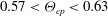 $0.57<{\it\Theta}_{cp}<0.63$
). (c) An avalanche is initiated by removing a portion of the floor, and the mean angle of repose is measured once the heap has stabilized; stable heap:
$0.57<{\it\Theta}_{cp}<0.63$
). (c) An avalanche is initiated by removing a portion of the floor, and the mean angle of repose is measured once the heap has stabilized; stable heap:
 $20^{\circ }<{\it\phi}_{r}<36^{\circ }$
. (d) Contour plot of the packing fraction (solid line) and angle of repose (dashed line (deg.)) as a function of the friction coefficients. The shaded region corresponds to acceptable friction coefficients for natural sands using the present model.
$20^{\circ }<{\it\phi}_{r}<36^{\circ }$
. (d) Contour plot of the packing fraction (solid line) and angle of repose (dashed line (deg.)) as a function of the friction coefficients. The shaded region corresponds to acceptable friction coefficients for natural sands using the present model.
During the initial phase of the simulation, an additional solid wall is placed just below the particles at
 $Y=0$
, and they settle onto this boundary under the action of gravity in water for a total time of 5 s (figure 18(b)). At this point,
$Y=0$
, and they settle onto this boundary under the action of gravity in water for a total time of 5 s (figure 18(b)). At this point,
 ${\it\Theta}_{cp}$
is computed by integrating the solid volume of all particles in the interior of the packing, those that are more than
${\it\Theta}_{cp}$
is computed by integrating the solid volume of all particles in the interior of the packing, those that are more than
 $4d_{50}$
from the bottom wall or the top granular surface.
$4d_{50}$
from the bottom wall or the top granular surface.
At
 $t=5$
s, the end sections of the solid wall, corresponding to a combined length of
$t=5$
s, the end sections of the solid wall, corresponding to a combined length of
 $L_{x}/4$
, are removed, initiating an avalanche of particles into the bottom half of the container. This process is allowed to proceed until
$L_{x}/4$
, are removed, initiating an avalanche of particles into the bottom half of the container. This process is allowed to proceed until
 $t=20~\text{s}$
to ensure that all particles have settled completely. The angle of repose is then taken as the average of the four angles
$t=20~\text{s}$
to ensure that all particles have settled completely. The angle of repose is then taken as the average of the four angles
 ${\it\phi}_{1},{\it\phi}_{2},{\it\phi}_{3},{\it\phi}_{4}$
produced by the avalanching process, shown in figure 18(c). To remove any influence of particle induced fluid motion on the static granular properties, a one-way coupling approach was used by setting
${\it\phi}_{1},{\it\phi}_{2},{\it\phi}_{3},{\it\phi}_{4}$
produced by the avalanching process, shown in figure 18(c). To remove any influence of particle induced fluid motion on the static granular properties, a one-way coupling approach was used by setting
 ${\it\Theta}_{p}=0$
and
${\it\Theta}_{p}=0$
and
 $\boldsymbol{f}_{p\rightarrow f}=0$
.
$\boldsymbol{f}_{p\rightarrow f}=0$
.
The test is repeated for 49 combinations of
 $\mathscr{V}_{s}$
and
$\mathscr{V}_{s}$
and
 $\mathscr{V}_{r}$
(
$\mathscr{V}_{r}$
(
 $\mathscr{V}_{s}=0.1$
, 0.2, 0.3, 0.4, 0.5, 0.6, 0.7 and
$\mathscr{V}_{s}=0.1$
, 0.2, 0.3, 0.4, 0.5, 0.6, 0.7 and
 $\mathscr{V}_{r}$
= 0.0, 0.02, 0.04, 0.06, 0.08, 0.10, 0.12). Other simulation parameters are held constant and are the same as in table 2. Variation of the friction coefficients results in a considerable range of results (
$\mathscr{V}_{r}$
= 0.0, 0.02, 0.04, 0.06, 0.08, 0.10, 0.12). Other simulation parameters are held constant and are the same as in table 2. Variation of the friction coefficients results in a considerable range of results (
 $0.57\leqslant {\it\Theta}_{CP}\leqslant 0.63$
,
$0.57\leqslant {\it\Theta}_{CP}\leqslant 0.63$
,
 $20^{\circ }\leqslant {\it\phi}_{r}\leqslant 36^{\circ }$
), which are shown in the in the
$20^{\circ }\leqslant {\it\phi}_{r}\leqslant 36^{\circ }$
), which are shown in the in the
 $\mathscr{V}_{s}$
–
$\mathscr{V}_{s}$
–
 $\mathscr{V}_{r}$
plane in figure 18(d). The shaded region corresponds to results consistent with the behaviour of natural sand, which leads to the selection of
$\mathscr{V}_{r}$
plane in figure 18(d). The shaded region corresponds to results consistent with the behaviour of natural sand, which leads to the selection of
 $\mathscr{V}_{s}=0.4$
and
$\mathscr{V}_{s}=0.4$
and
 $\mathscr{V}_{r}=0.06$
(marked by an X) for the simulations in § 4.
$\mathscr{V}_{r}=0.06$
(marked by an X) for the simulations in § 4.
A.3 Hindered settling dynamics
A successful simulation of sediment dynamics in the wave bottom boundary layer must faithfully capture sediment–fluid interactions over a wide range of solid fractions, from very dilute to the close-packed limit. In the present model, these interactions arise via the interphase momentum transfer term, the mixture viscosity and volume displacement effects. To confirm that the present combination of closures is consistent with known hindered settling behaviour (Richardson & Zaki Reference Richardson and Zaki1954), simulations of unbounded particle settling have been performed.
A triply periodic domain with
 $L_{x}=L_{y}=L_{z}=64d_{50}$
is chosen for the simulations and discretized with
$L_{x}=L_{y}=L_{z}=64d_{50}$
is chosen for the simulations and discretized with
 $64^{3}$
control volumes. Non-overlapping particles are seeded at random to obtain mean solid fractions in the range
$64^{3}$
control volumes. Non-overlapping particles are seeded at random to obtain mean solid fractions in the range
 $0.05\leqslant \langle {\it\Theta}_{p}\rangle \leqslant 0.6$
. Two sets of simulations are performed with uniform diameter glass beads (
$0.05\leqslant \langle {\it\Theta}_{p}\rangle \leqslant 0.6$
. Two sets of simulations are performed with uniform diameter glass beads (
 $d_{p}=0.35~\text{mm}$
) and beach sand (
$d_{p}=0.35~\text{mm}$
) and beach sand (
 $d_{50}=0.22~\text{mm}$
,
$d_{50}=0.22~\text{mm}$
,
 ${\it\sigma}_{g}=1.35$
), corresponding to the particle fluidization experiments of Baldock et al. (Reference Baldock, Tomkins, Nielsen and Hughes2004). The particle parameters are given in table 5. The other simulation parameters for the sand conditions are the same as used in § 4. The particles are initially at rest and settle under the action of gravity (
${\it\sigma}_{g}=1.35$
), corresponding to the particle fluidization experiments of Baldock et al. (Reference Baldock, Tomkins, Nielsen and Hughes2004). The particle parameters are given in table 5. The other simulation parameters for the sand conditions are the same as used in § 4. The particles are initially at rest and settle under the action of gravity (
 $g_{y}=-9.81~\text{m}^{-1}~\text{s}^{-2}$
), while a uniform body force is applied to the fluid (water) in the positive
$g_{y}=-9.81~\text{m}^{-1}~\text{s}^{-2}$
), while a uniform body force is applied to the fluid (water) in the positive
 $y$
direction to balance the weight of the particles. The simulations last for
$y$
direction to balance the weight of the particles. The simulations last for
 $30{\it\tau}_{st}$
, where
$30{\it\tau}_{st}$
, where
 ${\it\tau}_{st}=({\it\rho}_{p}d_{50}^{2}/18{\it\mu}_{0})$
is the isolated particle Stokes relaxation time of the median grain size, long enough for the (average) settling velocity to achieve a stationary value.
${\it\tau}_{st}=({\it\rho}_{p}d_{50}^{2}/18{\it\mu}_{0})$
is the isolated particle Stokes relaxation time of the median grain size, long enough for the (average) settling velocity to achieve a stationary value.

Figure 19. Hindered settling of a particle suspension under the action of gravity. (a) Particles coloured by instantaneous fall velocity for a mean solid fraction of
 $\langle {\it\Theta}_{p}\rangle =0.3$
. (b,c) Average particle settling velocity normalized by the single particle terminal velocity,
$\langle {\it\Theta}_{p}\rangle =0.3$
. (b,c) Average particle settling velocity normalized by the single particle terminal velocity,
 $v_{t,50}$
, as a function of
$v_{t,50}$
, as a function of
 $\langle {\it\Theta}_{p}\rangle$
. (b) Glass beads (
$\langle {\it\Theta}_{p}\rangle$
. (b) Glass beads (
 $d=0.35$
mm); (c) beach sand (
$d=0.35$
mm); (c) beach sand (
 $d_{50}=0.22$
mm), lognormal,
$d_{50}=0.22$
mm), lognormal,
 ${\it\sigma}_{g}=1.35$
. Comparisons are made with the Richardson & Zaki (Reference Richardson and Zaki1954) correlation and the experimental measurements of Baldock et al. (Reference Baldock, Tomkins, Nielsen and Hughes2004).
${\it\sigma}_{g}=1.35$
. Comparisons are made with the Richardson & Zaki (Reference Richardson and Zaki1954) correlation and the experimental measurements of Baldock et al. (Reference Baldock, Tomkins, Nielsen and Hughes2004).
Table 5. Particle and collision parameters used for the hindered settling tests.

In general, the particles do not all settle at the same velocity because they induce an unsteady flow and form clusters of fast and slow moving particles, as shown in figure 19(a) for the case of glass beads at
 $\langle {\it\Theta}_{p}\rangle =0.3$
. Each particle is coloured by its normalized settling velocity
$\langle {\it\Theta}_{p}\rangle =0.3$
. Each particle is coloured by its normalized settling velocity
 $v_{s}/v_{t,50}$
, where
$v_{s}/v_{t,50}$
, where
 $v_{t,50}$
is the unhindered terminal velocity of the median particle size.
$v_{t,50}$
is the unhindered terminal velocity of the median particle size.
The normalized particle settling velocity (in a frame in which the mean fluid velocity is zero) is averaged over all grains and plotted versus
 $\langle {\it\Theta}_{p}\rangle$
alongside the experimental data in figure 19(b,c). Also plotted is the empirical relationship of Richardson & Zaki (Reference Richardson and Zaki1954) for each condition. Overall, the agreement with experiments is excellent over almost the entire range of solid fractions for both mono-size spherical particles and sand with a natural size distribution, indicating that the current set of closures is appropriate.
$\langle {\it\Theta}_{p}\rangle$
alongside the experimental data in figure 19(b,c). Also plotted is the empirical relationship of Richardson & Zaki (Reference Richardson and Zaki1954) for each condition. Overall, the agreement with experiments is excellent over almost the entire range of solid fractions for both mono-size spherical particles and sand with a natural size distribution, indicating that the current set of closures is appropriate.
Appendix B. Model sensitivity
To assess the sensitivity of the model to the various model parameters, the transport of uniform-size sand particles under a steady turbulent flow is considered. An initial sand bed with depth
 $H_{bed}\approx 6~\text{mm}$
is created by allowing 112 916 particles with
$H_{bed}\approx 6~\text{mm}$
is created by allowing 112 916 particles with
 $d_{p}=0.44~\text{mm},~{\it\rho}_{p}=2650~\text{kg}~\text{m}^{-3}$
to settle under the action of gravity (
$d_{p}=0.44~\text{mm},~{\it\rho}_{p}=2650~\text{kg}~\text{m}^{-3}$
to settle under the action of gravity (
 $g_{y}=-9.81~\text{m}~\text{s}^{-1}$
) in water (
$g_{y}=-9.81~\text{m}~\text{s}^{-1}$
) in water (
 ${\it\rho}_{f}=1000~\text{kg}~\text{m}^{-3},{\it\mu}_{0}=0.001~\text{kg}~\text{m}^{-1}~\text{s}^{-1}$
) in a domain with
${\it\rho}_{f}=1000~\text{kg}~\text{m}^{-3},{\it\mu}_{0}=0.001~\text{kg}~\text{m}^{-1}~\text{s}^{-1}$
) in a domain with
 $L_{x}=128d_{p}$
,
$L_{x}=128d_{p}$
,
 $L_{y}=128d_{p}$
,
$L_{y}=128d_{p}$
,
 $L_{z}=64d_{p}$
. Particles that come into contact with the bottom wall are fixed, and a body force,
$L_{z}=64d_{p}$
. Particles that come into contact with the bottom wall are fixed, and a body force,
 $f_{x}$
, is then applied to the flow and particles in the
$f_{x}$
, is then applied to the flow and particles in the
 $X$
direction, so that the resulting Shields parameter is
$X$
direction, so that the resulting Shields parameter is
 ${\it\theta}={\it\rho}_{f}f_{x}(L_{y}-H_{bed})/({\it\rho}_{p}-{\it\rho}_{f})gd_{p}=0.5$
. The particle settling velocity is
${\it\theta}={\it\rho}_{f}f_{x}(L_{y}-H_{bed})/({\it\rho}_{p}-{\it\rho}_{f})gd_{p}=0.5$
. The particle settling velocity is
 $v_{s}=58~\text{mm}~\text{s}^{-1}$
, resulting in a suspension number of
$v_{s}=58~\text{mm}~\text{s}^{-1}$
, resulting in a suspension number of
 $\mathscr{S}=0.97$
, indicating a sheet flow at the transition between bedload and suspension mode (Sumer et al.
Reference Sumer, Kozakiewicz, Fredsøe and Deigaard1996).
$\mathscr{S}=0.97$
, indicating a sheet flow at the transition between bedload and suspension mode (Sumer et al.
Reference Sumer, Kozakiewicz, Fredsøe and Deigaard1996).
Table 6. Model sensitivity to simulation parameters. Baseline parameters are indicated in bold font, and mean transport rates are normalized by the baseline value (
 ${\it\Psi}_{b}=1.76$
).
${\it\Psi}_{b}=1.76$
).

The flow and particle transport are allowed to develop for 60 s using the baseline parameters given in table 2. The mean dimensionless particle transport is then computed for the next 30 s interval as
 $$\begin{eqnarray}{\it\Psi}=\displaystyle \mathop{\sum }_{particles}\frac{{\rm\pi}}{6}d_{p}^{3}u_{p,x}\bigg/L_{x}L_{z}\sqrt{\left(\frac{{\it\rho}_{p}}{{\it\rho}_{f}}-1\right)gd_{50}^{3}}.\end{eqnarray}$$
With the baseline parameters, a value of
 ${\it\Psi}_{b}=1.76$
is obtained. This lies between the value predicted by the Meyer-Peter & Müller (Reference Meyer-Peter and Müller1948) formula,
${\it\Psi}_{b}=1.76$
is obtained. This lies between the value predicted by the Meyer-Peter & Müller (Reference Meyer-Peter and Müller1948) formula,
 ${\it\Psi}_{mpm}=8({\it\theta}-0.047)^{3/2}=2.44$
, and the more recent correction proposed by Wong & Parker (Reference Wong and Parker2006),
${\it\Psi}_{mpm}=8({\it\theta}-0.047)^{3/2}=2.44$
, and the more recent correction proposed by Wong & Parker (Reference Wong and Parker2006),
 ${\it\Psi}_{wp}=3.97({\it\theta}-0.0495)^{3/2}=1.20$
. The sensitivity of the simulations is assessed by repeating the final 30 s of the simulation several times, changing only one parameter at a time, and examining any change to the mean transport rate.
${\it\Psi}_{wp}=3.97({\it\theta}-0.0495)^{3/2}=1.20$
. The sensitivity of the simulations is assessed by repeating the final 30 s of the simulation several times, changing only one parameter at a time, and examining any change to the mean transport rate.
Results are reported in table 6 as the ratio
 ${\it\Psi}/{\it\Psi}_{b}$
, to indicate the sensitivity to each parameter value change. The mean transport rate is found to depend very little, if at all, on the parameters
${\it\Psi}/{\it\Psi}_{b}$
, to indicate the sensitivity to each parameter value change. The mean transport rate is found to depend very little, if at all, on the parameters
 $k_{n}$
,
$k_{n}$
,
 $k_{t}$
and
$k_{t}$
and
 $e_{dry}$
. Considering dry collisions (
$e_{dry}$
. Considering dry collisions (
 $St_{c}=0,St_{e}=0$
) results in a 7 % higher transport rate, but using a somewhat wider transitional range,
$St_{c}=0,St_{e}=0$
) results in a 7 % higher transport rate, but using a somewhat wider transitional range,
 $St_{c}=11,St_{e}=130$
, increases the transport by less than 1 %. The frictional coefficients are found to have a weak effect, generally decreasing the transport with higher values. The intrinsic viscosity is found to have the strongest effect of any parameter on the transport rate. If mixture viscosity effects are neglected by setting
$St_{c}=11,St_{e}=130$
, increases the transport by less than 1 %. The frictional coefficients are found to have a weak effect, generally decreasing the transport with higher values. The intrinsic viscosity is found to have the strongest effect of any parameter on the transport rate. If mixture viscosity effects are neglected by setting
 $[{\it\mu}]=0.0$
, the transport rate increases by 44 %. A decrease of similar magnitude relative to the baseline can be realized by setting
$[{\it\mu}]=0.0$
, the transport rate increases by 44 %. A decrease of similar magnitude relative to the baseline can be realized by setting
 $[{\it\mu}]=5.0$
, corresponding to very angular particles (Ferrini et al.
Reference Ferrini, Ercolani, De Cindio, Nicodemo, Nicolais and Ranaudo1979), which underscores the importance of considering shape effects on bulk particle motion. The filter size does appear to have an influence on the results, but for
$[{\it\mu}]=5.0$
, corresponding to very angular particles (Ferrini et al.
Reference Ferrini, Ercolani, De Cindio, Nicodemo, Nicolais and Ranaudo1979), which underscores the importance of considering shape effects on bulk particle motion. The filter size does appear to have an influence on the results, but for
 $h\geqslant 2d_{p}$
, the sensitivity to
$h\geqslant 2d_{p}$
, the sensitivity to
 $h$
is minimized.
$h$
is minimized.


 Open access