


1 INTRODUCTION
Modern maps of radio continuum emission have tended towards increasing sensitivity and angular resolution. Increased sensitivity can be obtained with larger collecting area, but increased angular resolution normally means resorting to interferometers with widely spaced elements. Notable high-resolution, large-area interferometer surveys at radio wavelengths include SUMSS (Bock, Large, & Sadler, Reference Bock, Large and Sadler1999), FIRST (Becker, White, & Helfland, Reference Becker, White and Helfand1995), NVSS (Condon et al. Reference Condon1998), and AT20G (Murphy et al. Reference Murphy2010), which mapped the sky at frequencies from 843 MHz to 20 GHz.
However, interferometers are inherently insensitive to large-scale emission. That is, emission on angular scales greater than λ/Bs , where Bs is the shortest projected baseline, is lost. Whilst not an issue for discrete sources, this is a serious shortcoming for mapping large objects including: cluster halos; the lobes of giant radio galaxies; nearby supernova remnants and HII regions; and the diffuse thermal and non-thermal emission from the Milky Way and other nearby galaxies. Sensitive single-dish maps of the sky therefore remain useful for filling in the ‘missing information’, and can often be directly merged with interferometer maps of similar frequency and with overlapping coverage in the u-v domain.
Single-dish, single-beam millimetre wavelength continuum studies by the COBE, WMAP, and now Planck space missions have been spectacularly successful in mapping the Cosmic Microwave Background. Complemented by lower and higher frequency maps, to separate out thermal and non-thermal foregrounds, analysis of such maps have fundamentally improved the measurement accuracy of important cosmological parameters, e.g. Spergel et al. (Reference Spergel2003).
Recently, there has been renewed interest in low-frequency maps of the sky. This interest arises from the desire to: (a) constrain possible emission from spinning dust and large dust grains; (b) provide a low-resolution complement to all-sky maps from the Square Kilometre Array (SKA) pathfinders such as the Murchison Widefield Array (MWA) and LOFAR; and (c) provide missing polarisation information for characterising foreground emission, which contaminates EOR and CMB B-mode studies. The well-known map of Haslam et al. (Reference Haslam, Salter, Stoffel and Wilson1982) has stood out for many years as a low-frequency (408 MHz) reference map. However, it has fairly low resolution (0°.85), contains a number of artefacts, and has no polarisation information. It was a precursor to later studies including those at 1.42 GHz by Reich (Reference Reich1982), Reich & Reich (Reference Reich and Reich1986), Reich, Testori, & Reich (Reference Reich, Testori and Reich2001), and the 2.3 GHz S-PASS survey by Carretti (Reference Carretti, Kothes, Landecker and Willis2011). Unfortunately, these higher-resolution studies using single-beam receivers are expensive in telescope time—S-PASS took around 2 000 h of observing time on the Parkes telescope—and are therefore not straightforward to conduct.
Previous surveys that overlap the HI Parkes All-Sky Survey (HIPASS)/Zone of Avoidance (ZOA) coverage at frequencies close to 1.4 GHz and with resolution comparable to the $14\hbox{$.\hspace{-2.22214pt}^\prime $}4$
HPBW are: the all-sky survey at 408 MHz and 51 arcmin by Haslam et al. (Reference Haslam, Salter, Stoffel and Wilson1982); the 1.42 GHz surveys of Reich (Reference Reich1982) with + 20° < δ, Reich & Reich (Reference Reich and Reich1986) with − 19° ⩽ δ ⩽ +24°, and Reich et al. (Reference Reich, Testori and Reich2001) with δ < −10°, which between them cover the whole sky with HPBW 35 arcmin; the complementary polarisation surveys at 1.42 GHz of Wolleben et al. (Reference Wolleben, Landecker, Reich and Wielebinski2006) with − 29° < δ and Testori, Reich, & Reich (Reference Testori, Reich and Reich2008) with δ < −10°, each with HPBW 36 arcmin; and the 2.3 GHz survey of Jonas, Baart, & Nicolson (Reference Jonas, Baart and Nicolson1998) covering most of the range − 83° < δ < +32° with HPBW 20 arcmin. Wielebinski (Reference Wielebinski2009) provides a historical overview of these surveys.
$14\hbox{$.\hspace{-2.22214pt}^\prime $}4$
HPBW are: the all-sky survey at 408 MHz and 51 arcmin by Haslam et al. (Reference Haslam, Salter, Stoffel and Wilson1982); the 1.42 GHz surveys of Reich (Reference Reich1982) with + 20° < δ, Reich & Reich (Reference Reich and Reich1986) with − 19° ⩽ δ ⩽ +24°, and Reich et al. (Reference Reich, Testori and Reich2001) with δ < −10°, which between them cover the whole sky with HPBW 35 arcmin; the complementary polarisation surveys at 1.42 GHz of Wolleben et al. (Reference Wolleben, Landecker, Reich and Wielebinski2006) with − 29° < δ and Testori, Reich, & Reich (Reference Testori, Reich and Reich2008) with δ < −10°, each with HPBW 36 arcmin; and the 2.3 GHz survey of Jonas, Baart, & Nicolson (Reference Jonas, Baart and Nicolson1998) covering most of the range − 83° < δ < +32° with HPBW 20 arcmin. Wielebinski (Reference Wielebinski2009) provides a historical overview of these surveys.
The 408 MHz survey in particular has proved important for foreground subtraction of the WMAP CMB surveys at 23, 33, 41, 61, and 94 GHz (Hinshaw et al. Reference Hinshaw2007; Gold et al. Reference Gold2009), its 51 arcmin resolution being well-matched to the 23 GHz data. A resolution of 14.4 arcmin would be a better match to that of the higher WMAP frequency bands, and also to those of the Planck mission, which aims to achieve a final map of the CMB anisotropies in the vicinity of 5–10 arcmin.
The HIPASS and ZOA surveys were conducted using the 13-beam Parkes multibeam system starting on 1997 February 28, with HIPASS and its northern extension concluding on 2001 December 14, and ZOA with its extension into the Galactic bulge continuing until 2005 August 8. The raw data archive consists of 33 967 HIPASS and 15 305 ZOA scans, each of 100 × 5 s integrations, 13 beams, and 2 linear polarisations for an effective single-beam, single-polarisation equivalent total integration time of 640 Ms (~20 yrs). The multibeam instrumentation, HIPASS survey strategy, and data reduction software have been described by Barnes et al. (Reference Barnes2001), and the ZOA survey strategy by Staveley-Smith et al. (Reference Staveley-Smith1998).
Numerous papers based on this data set have been published, though to date these have been concerned almost exclusively with analysis of the 21 cm neutral hydrogen line [e.g. Meyer et al. (Reference Meyer2004); Zwaan et al. (Reference Zwaan2004)]. It has long been recognised that the survey data also contains a wealth of information on the hydrogen recombination lines between H166α and H168α. These are being studied in an ongoing series of papers by Alves et al. (Reference Alves, Davies, Dickinson, Calabretta, Davis and Staveley-Smith2012). It is also relatively simple to measure continuum flux densities for compact sources and studies have shown that it should be possible to measure spectral indices for the strongest of them (Melchiori et al. Reference Melchiori, Barnes, Calabretta and Webster2009). However, the task of producing large-scale continuum maps is complicated by a number of factors, the nature of which, and the solutions developed are the subject of this work.
In this paper, we introduce the surveys in Section 2 and extensively discuss all aspects of the data reduction in Section 3, including presentation of the final downloadable maps and comparison with previous studies. We briefly discuss the results in Section 4.
2 THE SURVEYS
For the purpose of this work the most important aspects of the survey strategy, summarised in Table 1, are:
-
• A central frequency of 1 394.5 MHz and bandwidth of 64 MHz in 1 024 spectral channels.
-
• The scan rate in each survey was 1 arcmin s−1 with 5 s integrations. The scan rate was used as part of the data validation as discussed in Section 3.1.
-
• HIPASS scanned in declination in 15 zones centred on declinations − 87°, and − 82° to + 22° in steps of 8°. The scan length was 8°.5 except for the shorter 4°.6 scans in the − 87° zone, and 7°.5 in the + 22° zone. The overlap between zones is significant for this work and is discussed in Section 3.7.
As the Parkes telescope is based on a master equatorial drive system, scans in the − 87° zone stopped just short of the south celestial pole (SCP), which consequently is surrounded by a small dead zone.
-
• The ZOA survey scanned in Galactic longitude in 27 zones centred on longitudes 200° to 48° in steps of 8°. The scan length was again 8°.5. Galactic latitudes between ± 5° were covered. In zones 336° to 32° the coverage was extended to ± 10°, and then to + 15° to cover the Galactic bulge in zones 352° to 16°. As the survey was designed primarily for detecting HI line emission, scanning was done in longitude rather than latitude in order to minimise the variation in Galactic continuum emission at 21 cm. By a quirk of geometry, this was a fortuitous choice for this work as well, as discussed in Section 3.7.
-
• Additional to HIPASS and ZOA, deep surveys were conducted of the Centaurus and Sculptor clusters of galaxies—HIDEEP (Minchin et al. Reference Minchin2003). The Centaurus survey comprised 623 scans centred on declination − 30° (excluding Cen A), so straddling the HIPASS − 34° and − 26° zones, whilst the 439 Sculptor scans lay entirely within the − 34° zone. These additional observations were used selectively as described.
-
• In each survey, the 13-beam multibeam feed array was rotated by 15° with respect to the scanning direction so that the beams were almost uniformly spaced on the sky, thus optimising coverage in a single scan. At the midpoint of a scan, the spacing between adjacent beams on the sky was then close to an integer multiple of 7 arcmin, just below the Nyquist rate of 5.7 arcmin viz {0, ± 8′, ± 13′, ± 21′, ± 28′, ± 36′, ± 49′}.
-
• The feed array was not rotated to account for parallactic effects once a scan had started, though parallactification was later found to have been enabled inadvertently for about 1% of the HIPASS scans.
In the completed HIPASS survey, the parallactic rotation in the course of a scan was found to be > 5° for 64% of the scans, > 10° for 29%, and > 15° for 9%. The corresponding figures for ZOA are 72%, 40%, and 22%. The effect this had on the mapping is discussed in Section 3.3.
-
• Adjacent HIPASS scans in the same zone are stepped by 7 arcmin orthogonal to the scan direction (i.e. in right ascension) so that each of the 13 beams mapped the sky at slightly below the Nyquist rate, whereby the survey is approximately ×10 oversampled spatially. However, because the step was close to the spacing between beams in an individual scan, the beam tracks in adjacent scans tended to overlay one another rather than fill in the spaces between them. The effect of this is discussed in Section 3.3.
-
• The scans in each HIPASS zone were organised into five interleaved sets (labelled a – d) with adjacent scans in each set stepped by 35 arcmin. Each interleave maps the sky at approximately twice the Nyquist rate and was completed before starting on the next. This ensured that scans for a particular part of the sky were observed at widely separated times, thus minimising the possible impact of Radio Frequency Interference (RFI), the Sun, Moon, and planets.
-
• Adjacent ZOA scans are stepped by 1.4 arcmin in Galactic latitude in 25 interleaved sets (a – y), i.e. ×5 denser than HIPASS.
-
• During observations, the system temperature was calibrated against a high-quality noise diode switched in and out of the signal path. The diode itself was calibrated periodically against a flux density calibrator, typically 1934-638 (14.9 Jy at 1 420 MHz) or Hydra A (40.6 Jy at 1 395 MHz, after correction for dilution in the beam of the telescope).
-
• The average system temperature at elevation 55° was 21°K. This rises towards higher elevations because of spillover effects, and likewise towards lower elevations with the additional contribution from atmospheric opacity becoming significant. Refer to Section 3.6.
Table 1. Summary of the survey parameters. Beam parameters are given for the central beam and the inner and outer rings of six beams each.

3 THE DATA REDUCTION
There were two main difficulties in extracting a 1.4 GHz continuum map of the sky from the 21 cm HIPASS data. The first was in correcting for the elevation dependence of T sys. A correction was derived from the HIPASS data itself in regions well away from Galactic emission as discussed in Section 3.6.
The second difficulty was that the zero level of each 8° HIPASS declination scan could only be determined by the narrow overlap between adjacent zones, with an arbitrary zero level for the sky as a whole. This is discussed in Section 3.7.
Firstly, however, there is the relatively simple but important step of removing invalid or questionable data from the HIPASS/ZOA data set.
3.1 Data validation
Whereas spectral line processing concerns the signal response in a few channels of a spectrum with a baseline defined by many, continuum processing is concerned with the many channels that define that baseline itself. Thus whilst spectral line processing is less sensitive to external variations in T sys, continuum processing is more sensitive and involves a certain element of dead-reckoning. For this reason extra care was taken to remove invalid data from the survey data sets.
An important test for validating HIPASS/ZOA data arises in connection with the way the Parkes telescope control system measures position in scanning observations. Positions are recorded at 5 s intervals with a separate timestamp that generally does not match the midpoint of the integration. Consequently, livedata Footnote 1 , the software that reads and processes the data, must buffer it and interpolate the positions to match the integration timestamp.
This position interpolation is based on a uniform scan rate, and as this is known beforehand to be 1 arcmin s−1, it provides a useful check on the positional accuracy.
However, in validating the scan rate, complications arise for the outer beams in a multibeam system due to grid convergence effects, particularly near the SCP. As the most extreme case, with the central beam at the pole and moving north, the beams on either side will have a non-zero motion in RA, either increasing or decreasing, with the trailing beams scanning towards the pole, i.e. in decreasing declination! Furthermore, because the feed array was not (usually) rotated to account for parallactic effects once a scan had started, a parallactic component of the scan rate arises for the outer beams, particularly for scans close to the zenith with a large change in azimuth.
Once these effects were accounted for, there was generally excellent agreement between the measured and nominal rates for all 13 beams within an allowed range of ±0.05 arcmin s−1 except for data that was genuinely discrepant. Of the latter a number of problems were readily identified:
-
• The first and last few integrations of a scan often reported discrepant scan rates. Often these were flagged as bad by the system but not always. For some scans it was apparent that the feed assembly had not quite finished rotating into position before the scan started.
It is important for this work that these integrations be culled; the overlap between zones used for level adjustment in Section 3.7 is normally limited to 11 integrations at most (23 for the − 87° zone), so two bad integrations could affect the results.
-
• Occasional (and rare) mid-scan glitches, apparently related to movement of the feed assembly or possibly a glitch in the feed rotation encoder or control system. Either way, the effect is to produce a questionable position, which thus necessitated culling of the affected integrations.
-
• A small number of scans were made with the wrong scan rate.
Detection of a bad scan rate resulted in all 13 beams × 2 polarisations being culled for the particular integration. The total number of integrations amounted to the equivalent of about 39 full scans but with bad integrations concentrated in the sensitive beginning and end integrations as discussed above.
The scan rate test also uncovered a number of correctable problems, some of which originated from causes that were understood, and others for which the cause could be reliably inferred. These data were corrected on-the-fly by livedata. This affected the equivalent of about 23 full scans.
Finally, in the process of validating and subsequently processing the data, an additional 227 complete scans were uncovered that needed to be culled for a variety of reasons, not necessarily relating to position or scan rate errors. For example, observations made with the wrong centre frequency or bandwidth. With the removal of these bad observations, 33 967 HIPASS and 15 305 ZOA scans remained.
After the data had been completely processed, it became apparent that the results were affected by sources that were strong enough to saturate the receiver electronics. This was particularly so for the classical radio sources such as Sgr A, Tau A, Ori A, Cen A, etc. In HIPASS/ZOA spectral processing, integrations were culled by the reader if all beams and polarisations were flagged because of saturation. However, partially flagged integrations were allowed to pass through the bandpass calibration phase and only culled when the data was gridded into spectral cubes. Again, a more rigorous treatment was required for continuum processing, with the bandpass calibration phase modified to handle partially flagged data properly.
3.2 Bandpass calibration
The bandpass calibration algorithm described by Barnes et al. (Reference Barnes2001) was modified for continuum processing in several key respects.
-
• In representational terms, HIPASS/ZOA bandpass calibration was based on the following equation, which is applied in turn to each spectral channel:
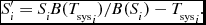
Here Si and S′ i are the raw and calibrated values in the spectral channel for integration i, and B(), estimates the baseline response for a quantity that varies with i (because of scanning), whether T sys i or Si . In essence, B() determines the baseline in source-free (reference) regions of the scan and interpolates into the integrations occupied by sources. In HIPASS/ZOA it was implemented as a running-median filter.(1) \begin{equation}
S^{\prime }_i = S_i B({T_{\mathrm{sys}}}_i) / B(S_i) - {T_{\mathrm{sys}}}_i .
\end{equation}
\begin{equation}
S^{\prime }_i = S_i B({T_{\mathrm{sys}}}_i) / B(S_i) - {T_{\mathrm{sys}}}_i .
\end{equation}
Equation (1) is applied in turn to each of the 1 024 channels, separately for each of the 13 beams × 2 polarisations.
Besides receiver noise, T sys i contains the signal from cosmic continuum emission. By subtracting it, the continuum is thereby discarded. Instead we use
Here we have only subtracted the base-level value of T sys i , which should consist of receiver noise only, thus preserving the cosmic signal of interest.(2)
\begin{equation}
S^{\prime }_i = S_i / B(S_i / {T_{\mathrm{sys}}}_i) - B({T_{\mathrm{sys}}}_i)
\end{equation}
Note in Equation (2) that each spectrum is first divided by T sys as a prelude to bandpass calibration in order to avoid statistical biasses that may be introduced by integrations affected by strong continuum emission. That is, the scale factor is 1/B(Si /T sys i ), not B(T sys i )/B(Si ).
Note also that the factor is not B(T sys i /Si ) as can be understood simply by considering that integrations could conceivably have Si = 0 in channels close to the edge of the band, whereas T sys i > 0 always.
-
• 21 cm continuum emission extends over many degrees, often exceeding the 8° scan length. However, as discussed by Putman et al. (Reference Putman, Staveley-Smith, Freeman, Gibson and Barnes2003), the HIPASS/ZOA compact source algorithm is designed for extragalactic objects of typically < 1° in extent and is blind to regions of emission much larger than this.
Figure 1 Footnote 2 shows the result of applying a compact source algorithm to continuum data. The algorithm differed from the running median used by HIPASS/ZOA, instead utilising a robust polynomial fitting technique as described in McClure-Griffiths et al. (Reference McClure-Griffiths2009). Most of the extended emission is lost, leaving behind only point sources and ridges. Such maps are useful in their own right for producing point-source catalogues.
Figure 1. HIPASS ‘point-source’ continuum map at 1.4 GHz produced using the HIPASS/ZOA compact source algorithm, which is sensitive only to regions of emission much less than 8° in extent. The high-pass spatial filter also produces pronounced negatives on either side of the Galactic plane. This map and those following are on a Hammer-Aitoff projection in Galactic coordinates centred on (ℓ, b) = (0°, 0°) at which point the pixel spacing is 4 arcmin in either direction. Longitude increases towards the left as usual for a celestial map. A three-cycle logarithmic base-10 intensity scale is used for this and the following images; the greyscale range is 0.05–50 Jy beam−1 (nominal calibration).
For their work on the Magellanic stream and high-velocity clouds, which have scales extending well beyond 1° in size, Putman et al. (Reference Putman, Staveley-Smith, Freeman, Gibson and Barnes2003) used the minmed5 algorithm for function B() in Equation (1). For each spectral channel, the scan is divided into five fixed segments 1°.6 in length and the median of the ~20 integrations computed for each. The segment with the lowest response of the five is then used as the zero level for the whole scan.
This work uses a refinement of minmed5. Instead of five fixed segments, the running median in a box of chosen size is computed for the whole scan. Ideally the box should be small, but not so small as to be affected by the intrinsic noise associated with extremal statistics. In practice, a box of size 10 integrations, being half that of minmed5, was found to be an acceptable compromise. This means that we should expect a minimum of 5 negative integrations per channel, rather than 10, out of the 100 integrations in a bandpass-calibrated scan.
This running-median technique provides the bandpass calibration function B() in Equation (2).
-
• In the post-bandpass calibration phase, a robust polynomial fit of degree four (quartic) is done over frequency for each spectrum in a scan. The robust polynomial fitting algorithm used by livedata has been described by McClure-Griffiths et al. (Reference McClure-Griffiths2009). In this instance an initial mask 41 channels wide was set to exclude Galactic HI emission.
The continuum response is defined by the zeroth and first order coefficients of the best-fit polynomial, the latter providing a measure of the spectral index; the continuum flux density varies by ~10% across the 64 MHz band at 1394.5 MHz for a source with α = ±2.

The map shown in Figure 2 is the result of applying the running-median bandpass calibration technique. It illustrates the two effects requiring calibration. Firstly the elevation dependence of T sys, which manifests itself as an apparent increase in continuum emission towards lower elevations, here the celestial equator and SCP. This is discussed in Section 3.6. Secondly the discontinuity along the edges of the 8° declination zones. Zone-level adjustment, required to eliminate this, is discussed in Section 3.7.

Figure 2. HIPASS 1.4 GHz continuum data now processed with the running-median algorithm, which is sensitive to extended emission. The 15 HIPASS declination zones are readily apparent. This map illustrates the two effects requiring calibration: the elevation dependence of T sys discussed in Section 3.6, which produces the gradual brightening away from the zenith, and the zone-level adjustment discussed in Section 3.7, which delineates the 15 declination zones. Same logarithmic greyscale as Figure 1.
3.3 Gridding
Whilst map production is normally the last step in data processing, this work relied on various forms of gridding at all stages of the reduction. Two intermediate maps have already been shown in Figures 1 and 2. Therefore it is appropriate to discuss gridding at this point.
The large number of gridding techniques in common use—kriging, minimum curvature, Delaunay triangulation, bi-directional line, thin plate spline, inverse distance weighted, etc.–suggests that there is no single general method that suits all purposes. Many of these gridding algorithms are designed for sparse, well-determined measurements, such as pertain in the geospatial fields, where the problem is to interpolate from an irregular to a regular grid. On the contrary, we are faced with a large, over-determined data set, which, however, is subject to measurement error and may have severe outliers. Use of a robust statistical gridding technique is therefore indicated.
Barnes et al. (Reference Barnes2001) describe the robust gridding algorithm used to produce the final HIPASS/ZOA spectral cubes as implemented by gridzilla Footnote 3 . For this work, adaptations were required to handle very wide fields of view correctly, to implement the FITS celestial and spectral world coordinate systems (Greisen & Calabretta, Reference Greisen and Calabretta2002; Calabretta & Greisen, Reference Calabretta and Greisen2002; Greisen et al. Reference Greisen, Calabretta, Valdes and Allen2006), and to deal with the much larger amount of input data and output image size.
Another significant change in this work was in the gridding statistic used. As the beam normalisation applied by Equation (5) of Barnes et al. (Reference Barnes2001) is not appropriate for extended emission, their Equation (8) was replaced by a weighted median estimator that is equally robust against RFI and other time-variable sources of emission such as the Sun, Moon, and planets.
The weighted median is the middle-weight value—the sum of weights of all measurements less than it being equal to that of all measurements greater. Pro rata interpolation is used to bisect the sum of weights if required. This statistic is a generalisation of the median in the same way that the weighted mean generalises the mean. To see this, first consider the case where all weights, wi , are integral. Computation of the weighted mean and median is then equivalent to replacing each measurement xi with weight wi by wi measurements of value xi and computing the unweighted mean or median in the usual way. For non-integral weights, each weight may be replaced by an integral approximation ⌊wi 10 k ⌋ and the limit taken as k → ∞.
As previously described, HIPASS scanned in declination alone, in general there are no orthogonal scans with which to form a ‘basket-weave’ (Sieber, Haslam, & Salter, Reference Sieber, Haslam and Salter1979; Emerson & Gräve, Reference Emerson and Gräve2009). Normally one would expect to see noticeable striping in maps produced from such data. However, two factors mitigate against this in HIPASS: the ×10 oversampling above the Nyquist rate, and parallactic rotation of the outer beams. The latter means that the outer beams do not actually scan in declination but instead follow a path that either tends to converge on the central beam or diverge from it. Consequently, when the tracks from all scans that contribute to a particular patch of the sky are mapped, the result tends to be a jumble of obliquely intersecting lines rather than a parallel array, as shown in Figure 3.

Figure 3. HIPASS beam tracks within ±0°.5 of arc of RA = 12h in the + 22°, − 42°, and − 82° declination zones. The effect of parallactic rotation of the outer beams is evident in this equi-scaled, equiareal Sanson-Flamsteed projection. The ‘windows’ near the centre of the scan arise because the rotation angle of the multibeam feed assembly was tuned for this point. Superposed on the tracks, the 14.4 arcmin HPBW is represented as the outer diameter of the central black circle whose inner diameter corresponds to the 6 arcmin radius cut-off in the gridding kernel used in HIPASS spectral line processing. A pair of RA meridians is superposed in grey to indicate grid convergence towards the poles; the central beam follows such a track. Dots on the tracks indicate sample points.
As seen in Figure 3, parallactic rotation in the + 22° zone is minimal and increases progressively towards the southern zones. The + 22° zone is just above the elevation limit of the Parkes dish; in fact the last degree or so is below the limit and the scans are truncated. Consequently, these northerly scans are performed mainly in elevation on the local meridian, the change in azimuth being limited to that required to follow diurnal rotation. Since the parallactic angle generally changes more quickly with azimuth than elevation, parallactic rotation of the outer beams is thereby minimised.
Because the step size of 7 arcmin between scans matches the basic separation between the beams in an individual scan, the beam tracks of successive scans tend to overlay one another. This creates a raster pattern that is more pronounced closer to the equator and near the midpoint of the scans, but tends to be obliterated by parallactic rotation in the more southerly zones as is shown in Figure 3. The raster was of little consequence for HIPASS spectral line processing, which was concerned with compact sources, and beam normalisation probably also helped to obscure it. In fact, it might be considered advantageous to have all 13 beams contribute equally to each point in the map. However, the raster does manifest itself, albeit at a low level, in various parts of the continuum map because of the extended scale of the emission.
3.3.1 Iterative gridding
Weighted median gridding is a non-linear process. It has the desirable property of robustness against outliers such as might arise from RFI, the Sun, Moon, or satellites. With the parameters typically used, it also tends to produce a gridded beam that is very close to Gaussian with FWHM that is remarkably insensitive to the cut-off radius, i.e. the radius of the circular ‘catchment area’ surrounding each pixel in the map. For example, in simulations using a circular Gaussian of FWHM 14.40 arcmin and a cut-off radius of 6 arcmin, the gridded FWHM was measured at only 14.45 arcmin, increasing to only 14.90 arcmin for a cut-off of 12 arcmin.
However, as explained in Barnes et al. (Reference Barnes2001), one adverse effect of median gridding is that the flux density scale differs depending on the source size. Without beam normalisation, compact sources appear in the map with reduced peak height, whilst extended sources appear at their correct peak height. Whilst this is also true of mean gridding, in that case the volume is preserved via broadening of the gridded beam, whereas with median gridding it is not because the gridded beam is not significantly broadened. The magnitude of the effect on compact source peak height depends on the gridding parameters, particularly the cut-off radius.
Unless otherwise stated, the simulations referred to below were done using a top-hat kernel, natural (unity) beam weighting, and without beam normalisation. For HIPASS data, with cut-off = 6 arcmin, point sources appear with peak height of about 86% their true value. With a 12 arcmin cut-off radius this quickly degrades to 61%. Whilst compact sources can be corrected by beam normalisation (as used in HIPASS), this inflates, and could introduce other adverse effects for extended sources. On the other hand, if a map consists only of extended sources then there is no problem. However, the all-sky continuum map is composed of extended and compact emission of equal import.
Iteration provides a solution to this problem for maps that contain a mix of compact and extended sources. Initially the zeroth-iteration map (henceforth 0-iter) is produced as normal. In the first iteration, the 0-iter map is subtracted from the raw data, which is then gridded to produce a residual map. Compact and slightly extended sources, which were underestimated in the 0-iter map, will be recovered, at least partially, in the residual map, which is then added to the 0-iter map to produce the first-iteration map (1-iter). Further iterations may be performed in like vein.
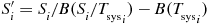
As the raw data serves as the standard against which the map in each iteration is compared, gridzilla never modifies it after reading it into memory. There is also too much of it to make a full working copy. Instead, each datum has the map value from the previous iteration subtracted only at the point that it is used, and as most data contributes to several pixels this happens multiple times for each datum. Iterative gridding thus requires a fast and accurate interpolation method for a practical implementation. gridzilla uses barycentric bivariate parabolic interpolation (Rodríguez et al. Reference Rodríguez2012) on the nine nearest pixelsFootnote 4 . In its general form
 \begin{eqnarray}
f(x,y) & = & \sum _{i=1}^{3}\sum _{j=1}^{3} f(x_i,y_j) \left[ \frac{p_i(x) p_j(y)}{p_i(x_i) p_j(y_j)} \right], \nonumber \\
p_i(x) & = & \prod _{k=1,k \ne i}^{3} (x - x_k),
\end{eqnarray}
\begin{eqnarray}
f(x,y) & = & \sum _{i=1}^{3}\sum _{j=1}^{3} f(x_i,y_j) \left[ \frac{p_i(x) p_j(y)}{p_i(x_i) p_j(y_j)} \right], \nonumber \\
p_i(x) & = & \prod _{k=1,k \ne i}^{3} (x - x_k),
\end{eqnarray}
Iteration may also be used productively for mean gridding where it acts to reduce the gridded beam size. Effectively, by driving the residual map towards zero, it makes the gridded map look more like the data in the sense that if the raw data were plotted on the map they would sit close to the surface defined by it.
Iteration in gridzilla is performed after the data has been indexed and read in and so adds only a relatively small overhead in processing time. It can also be sped up by applying a gain factor to the residual map before adding it. This factor compensates for the fact that point sources will appear in the residual map still with underestimated peak height. If the factor used is too high then when the corrected map is subtracted from the raw data it might drive some of it negative. However, negatives appearing in the residual map on the next iteration would then tend to correct this.
However, it is important to chose the gain factor appropriately to minimise the number of iterations, preferably to just one, because the base-level noise increases steadily with each successive iteration. This can be understood by considering a map produced from data that consists solely of noise. Because of the averaging associated with statistical gridding and the fact that the noise in the data is spatially uncorrelated, the root mean square (rms) noise in the 0-iter map will be much less than in the data (about 10% for a 6 arcmin cut-off). Therefore, subtracting the 0-iter map from the data will change it only weakly, whence the residual map will be highly correlated with the 0-iter map, i.e. the noise pattern will be similar. Thus when the residual is added to the 0-iter map the noise tends to be significantly worse than the sum in quadrature expected for uncorrelated noise. In simulations performed with a 6 arcmin cut-off, the rms noise in the 1-iter map was 50% higher than the 0-iter map for both mean and median. For the next two iterations the rms increased by roughly 20% per iteration.
However, because the residual map is only added to correct the profile of sources in the map, it only makes sense to add those parts of the residual map that do in fact achieve this. The rest is set to zero via a censoring algorithm. The residual values for a pixel and its eight neighbours are summed, giving half-weight to those in the corners. If this sum is below ×1.5 the map rms the value is zeroed, i.e. the nine pixels must be a little above twice the rms on average. This criterion helps to exclude isolated noise spikes, and to retain weak residuals in the vicinity of strong ones, i.e. on the edge of sources. Whilst this censoring ameliorates the adverse noise behaviour of iterative gridding on the background regions, it does tend to complicate the noise characteristics of the map as a whole.
Considering the unfavourable noise behaviour of iterative gridding, it is indeed fortunate that only a single iteration is required to achieve high-precision results for typical gridding parameters. If point sources appear in the 0-iter map at ratio g of their true peak height, then they would be expected to appear in the 1-iter map at ratio g + g(1 − g)f, where f is the loop gain factor. A factor f = 1.16 is thereby indicated for g = 86% (as above). However, this factor only applies to point sources—slightly extended sources would be overestimated. Sources that appear in the 0-iter map at ratio h (>g) will appear in the 1-iter map at r = h + h(1 − h)f. The worst case occurs for h = (1 + f)/2f. With f = 1.16 here, h = 0.93, whence r = 1.006, i.e. a precision of 0.6%.
In simulations using HIPASS data with a 6 arcmin cut-off, the integrated flux density and peak height of Gaussian test sources of various sizes were indeed recovered to within 1% with a single iteration using a gain of 1.2 for both the median and mean. In fact, acceptable results, to within about 3%, were obtained with gain factors in the range 1.1 to 1.3. The implied HPBW, i.e. $\sqrt{(}F^2 - T^2)$
where F is the measured FWHM and T = 14.4 arcmin is the FWHM of the test source, was 14.3 arcmin for median gridding (indicating a slight tendency to super-resolve), and at 14.6 arcmin was only slightly greater than it for mean gridding.
$\sqrt{(}F^2 - T^2)$
where F is the measured FWHM and T = 14.4 arcmin is the FWHM of the test source, was 14.3 arcmin for median gridding (indicating a slight tendency to super-resolve), and at 14.6 arcmin was only slightly greater than it for mean gridding.
Minor edge effects are associated with iterative gridding because spectra that contribute to edge pixels, though lying outside the map, cannot be reliably corrected. The width of the edge strip affected is slightly greater than the cut-off radius.
3.4 Robust measures of dispersion
As previously stated, the HIPASS/ZOA data set contains severe outliers arising from RFI, the Sun, Moon, and satellites. Rather than attempting to censor the data, robust statistical methods are used to ameliorate their effects. Principal amongst these methods is the use of the weighted median in place of the mean when estimating an average value.
Whilst the Gaussian asymptotic efficiencyFootnote 5 of the median is only 64% with respect to the mean [increasing marginally for sample sizes less than nine, Snedecor & Cochran (Reference Snedecor and Cochran1989)], the efficiency of the median absolute deviation from the median (mad),
 \begin{equation}
\mathrm{MAD} = 1.4826 \mathrm{med}_i |x_i - \mathrm{med}_j x_j|,
\end{equation}
\begin{equation}
\mathrm{MAD} = 1.4826 \mathrm{med}_i |x_i - \mathrm{med}_j x_j|,
\end{equation}
 \begin{equation}
S_n = 1.1926 \mathrm{med}_i[\mathrm{med}_j(|x_i - x_j|)].
\end{equation}
\begin{equation}
S_n = 1.1926 \mathrm{med}_i[\mathrm{med}_j(|x_i - x_j|)].
\end{equation}
In this work, Sn is always used in place of the rms whenever a measure of dispersion is required. Sn has a higher computational cost than the mad but that is irrelevant here. Croux & Rousseeuw (Reference Croux, Rousseeuw, Dodge and Whittaker1992) describe an O(nlog n) algorithm and provide an implementation in Fortran. This source code was translatedFootnote 6 to C for use by livedata and gridzilla.
3.5 Continuum baseline signature
A portion of the signal from a cosmic radio source may undergo multiple reflections from the structure of the Parkes radio telescope before being detected. Principal amongst these is the reflection from the base of the prime focus cabin that returns to the receiver after secondary reflection from the dish. Constructive or destructive interference with the primary signal may occur depending on the frequency and this gives rise to a ripple pattern of small relative amplitude in the spectral response of strong continuum sources. The period of this ripple corresponds to twice the distance from the base of the feed cabin to the dish, which is a little less than the focal length of 27.4 m. At Parkes the ripple has a period of 5.7 MHz, thus with 11 full cycles in the 64 MHz bandwidth. In reality, the ripple pattern is not a pure sinusoid, being complicated by reflections from the feed legs as well.
As discussed by Barnes et al. (Reference Barnes2001), Solar emission is the most common cause of ripple within individual scans taken during daylight hours. However, as it is a moving celestial source, the Sun differently affects spectra taken at a particular point in the sky at different times and its influence does not survive robust gridding (Section 3.3). This is not the case for strong, fixed cosmic continuum sources such as Sgr A and a host of other Galactic and extra-Galactic sources whose effect is constant for each scan. We distinguish between ripple caused by sources close to the optical axis of the telescope, which has a fixed pattern (Section 3.5.1), and that caused by sources away from the optical axis, which does not (Section 3.5.3).
In addition to the baseline ripple, Barnes et al. (Reference Barnes2001) also reported that the multibeam receivers exhibit a frequency-dependent response that results in an accelerating rise in the continuum response towards low frequencies (Section 3.5.2). Like the baseline ripple, this effect is also proportional to the strength of the continuum source.
Whilst these baseline effects pose significant problems for spectral line observations, they are also a nuisance factor for continuum work. Barnes et al. (Reference Barnes2001) described measures taken to correct the gridded maps, and also speculated that future reprocessing might correct the individual spectra before gridding. That approach is to be preferred as the ripple and curvature response, hereafter continuum baseline signature or CBS, varies with beam and polarisation and so are best removed before the spectra are combined in the gridded map.
The work reported in this section is also of particular interest to two current projects involving the HIPASS/ZOA data set, that of extracting hydrogen recombination line (RRL) maps (Alves et al. Reference Alves, Davies, Dickinson, Calabretta, Davis and Staveley-Smith2012), and of reprocessing the HIPASS/ZOA survey itself using improved techniques (Koribalski et al. in preparation).
3.5.1 On-axis ripple
The scaled template method of correcting the CBS described by Barnes et al. (Reference Barnes2001) relied on the first-order constancy of the shape of the CBS. For each data cube, the first step was to determine the normalised CBS empirically from the spectra of strong continuum sources. Then for each spectrum in the cube, the appropriate scale factor was measured directly from the data and the scaled template CBS subtracted.
Essentially the same method is used here, the difference being that the normalised CBS is determined separately for each beam and polarisation, this being done once and for all using a large subset of the HIPASS survey data. The appropriately scaled template CBS is then subtracted from each spectrum by livedata during post-bandpass processing.
To determine the CBS templates, the entire HIPASS/ZOA data set was reprocessed using robust polynomial bandpass calibration, with the continuum preserved as per Section 3.2, but without Doppler shifting nor spectral baseline removal. Preliminary investigation found that the CBS is produced only by point sources, extended continuum emission makes no contribution and so interferes with the normalisation of the spectra by the continuum level. Nor could any significant dependence on elevation nor feed rotation angle be discerned. Consequently, in order to exclude strong extended emission in the Galactic plane, only a subset of the HIPASS data with |b| > 15° was used to derive the CBS templates. For each beam and polarisation, using only spectra with a continuum level of at least 0.25 Jy beam−1, the spectra were normalised by the measured continuum level, and the template then formed as the weighted median of these normalised spectra, with the continuum flux density used as the weight.
Galactic HI emission was mostly removed from the CBS templates by taking advantage of the annual Doppler shift, which pushes the line around sufficiently so that each of the relevant channels is unaffected for at least part of the year. The number of spectra used to generate the templates varied between 74 062 and 120 000 spectra depending on beam (mainly) and polarisation. This number greatly exceeds that used in the original HIPASS processing with a consequent reduction in the noise to the extent that small birdies became visible. These were removed via a nine-point running median smooth as was done by Barnes et al. (Reference Barnes2001).
3.5.2 Baseline curvature
Having derived the CBS templates, the task remains of determining the appropriate scaling factor for removing the CBS from each individual spectrum.
Preliminary investigation revealed that simple scaling of the template CBS by the continuum level, measured as the median value of the spectrum (excluding Galactic HI), was adequate for weak sources for which the correction is barely significant anyway. However, a small residual of the ripple component often remained for very strong sources. Strong, extended continuum emission is a complicating factor as it increases the continuum level without augmenting the CBS.
A different, more computationally intensive strategy was therefore adopted for the 10% of spectra with a continuum level of 1 Jy beam−1 or stronger. This method optimised removal of the ripple component at the expense of possibly leaving a small residual of the curvature component, which, however, could easily be removed later with a polynomial baseline fit. The first step therefore was to separate the ripple from the baseline curvature component.
The ripple has a basic frequency of 5.7 MHz, which corresponds to 91 channels in the HIPASS/ZOA spectra. Applying a running mean of this width to the CBS templates therefore removes the ripple leaving behind only the curvature component. The ripple component may then be recovered by subtracting the curvature component from the CBS. This decomposition is shown in Figure 4.

Figure 4. Continuum baseline signature (CBS) templates for each beam and polarisation decomposed into the ripple (left) and curvature components (right). Channel 1 024 is the low frequency end. Beam 1 is at the bottom and successive beams are offset by 0.02 as indicated by the dashed horizontal lines. The two polarisations are shown for each beam as black and grey traces. For the ripple component there is such a close correspondence between them that the two traces are often indistinguishable.
For stronger sources, the scale factor for the CBS template was determined from the ripple component alone. A nine-point median smooth was applied to the spectrum being corrected to match what was done in deriving the CBS templates. This eliminates H-recombination and narrow RFI lines and reduces the noise a little. Smoothing with a running mean over 91 channels then removes the ripple, leaving only the baseline which was then subtracted from the spectrum to isolate the ripple component. This was then divided by the template ripple component shown in Figure 4, and the scale factor determined as the weighted median, with the weight taken as the ripple template value. In fact, RFI that occupies up to one-quarter of the band can significantly affect the computation of the median across the whole band so this potential source of contamination was minimised by taking the median of the medians of each three-quarters of the band.
As expected, spectral cubes produced from data processed with this method of CBS removal compare favourably with the older scaled template method. Because separate templates are used for each beam and polarisation, the ripple is more effectively removed. The baseline noise is also significantly reduced because the CBS templates are constructed from a much larger number of spectra and consequently are virtually noise-free. Also, because the CBS correction is applied before gridding, rather than after, there is less scatter in the data used to compute each pixel value in the gridded cube.
3.5.3 Off-axis ripple
As we have seen, strong on-axis point-source continuum emission creates highly reproducible baseline distortions that can be characterised and removed. Not so for strong off-axis continuum sources, which often manifest themselves via irregular, quasi-periodic baseline disturbances that evolve with position as the telescope scans. Principal amongst these is the Sun, which may affect daytime observations. Although it has a variable effect for each specific point on the sky and so does not survive robust gridding, nevertheless any increase in the scatter in the data acts to reduce the accuracy of the final result. On the other hand, strong fixed cosmic continuum sources, of which there are many, especially in the Galactic plane, have a static effect, which can survive robust gridding. Thus for spectral line work it is always advantageous to remove such baseline distortions as far as is practicable, although with no benefit at all for continuum work.
When the scan for a particular beam and polarisation is represented as an image of channel versus position (i.e. time for a scanning observation), off-axis ripple manifests itself as an irregular, quasi-periodic pattern, usually with harmonics oriented at an angle to the horizontal or vertical as seen in Figure 5a. This suggests the use of a low-pass 2D Fourier filter to model the ripple pattern.

Figure 5. Steps in off-axis ripple filtering. The spectral axis has frequency decreasing to the right from 1426.5 to 1362.5 MHz; the vertical axis is scan position, 500 s or equivalently 500 arcmin in extent: (a) the uncorrected scan; (b) masking of channels containing Galactic HI and RFI, as well as isolated discrepant pixels; (c) after linear interpolation and nine-point median smoothing in each direction; (d) masked pixels in (b) replaced with those of (c) after low-pass Fourier filtering; (e) ripple model obtained by low-pass Fourier filtering of (d); finally, (f) the corrected scan obtained by subtracting (e) from (a).
The principal difficulty is that such filtering is not robust against strong RFI nor line emission, which must therefore be excised. Figure 5 shows schematically the steps involved. Because the ripple pattern is broad-scale, whereas the RFI or line emission usually occupies a narrow range of channels or integrations, the strategy is to interpolate across it.
Bandpass calibration effectively ensures that the mean value in each spectral channel is close to zero. However, line emission and RFI still clearly manifest themselves via the dispersion, as seen in Figure 5a. As a prelude, isolated narrow- and broad-band RFI transients are masked on a channel-by-channel basis by censoring pixels outside 3×Sn for the channel, where Sn is the robust measure of dispersion discussed in Section 3.4. This discriminant corresponds to 3σ for a normal distribution. As it is not sufficient simply to zero these pixels, their values are replaced by linear interpolation across neighbouring values.
Discrepant channels are then identified by a discriminant based on the dispersion of the dispersion, i.e. channels that have a value of Sn much higher than normal, such that they correspond to 4σ outliers. The channel mask is then broadened by flagging immediately neighbouring channels if they have Sn outside 1σ. Linear interpolation across the channels provides values for the masked channels, followed by nine-point median smoothing to eliminate any small patches of narrow RFI that may have survived to this point, as in Figure 5c. This first-pass interpolation is then subjected to low-pass Fourier filtering using a Gaussian filter function with twice the FWHM of the required final filter function. The result is used to provide values for the masked pixels in the original unsmoothed image, and this then subjected to low-pass Fourier filtering to obtain the ripple model as in Figure 5e.
A Gaussian with FWHM of 16 harmonics in the spectral direction and 8 in the scanning direction proved to be an acceptable compromise for removing the ripple whilst retaining compact spectral line sources, though inevitably creating shallow moats around them.
3.6 T sys elevation dependence
T sys increases systematically towards lower elevations due to a combination of increasing atmospheric opacity and increasing spillover as distant sidelobes intersect with the ground. As is apparent in Figure 2, this effect is more pronounced in the northern declination zones because T sys changes more rapidly at lower elevations, and because scans in these zones are predominantly in elevation.
As elevation, η, increases from its lower limit, T sys drops to a minimum at about η = 58° and thereafter increases in a somewhat irregular way towards the zenith because of spillover effects. This is not apparent in Figure 2 because the declination zones that can be observed at elevations above 58° can also be observed at lower elevations where the scans may be predominantly in azimuth. Moreover, HIPASS/ZOA observations tended to be made at elevations away from the zenith in order to limit the change in parallactic angle. Consequently the effect is washed out. Nevertheless, it must contribute noise to the map.
Figure 2 shows that the elevation dependence of T sys has an obvious signature, which implies that it should be possible to deduce a correction from the HIPASS data itself. The Galactic plane and various other strong, large-scale emission features that might contaminate the results were excluded from the analysis; Table 2 indicates the RA ranges used. Unfortunately, the north-polar spur and other large features precluded using long stretches of the northern zones. Whilst low level emission is also evident even in the selected regions, we rely on the essentially random distribution of observations to cancel it out. That is, if we consider all of the observations made at a particular elevation, there are likely to be as many cosmic emission features that contribute a positive gradient as a negative gradient. The effect then is to add statistical noise. In any case, this approach is likely to produce more accurate results than traditional sky-dips, which are likely to traverse the same emission features, albeit unknowingly.
Table 2. Regions used to determine T sys(η, ζ), and (below) as represented on a plate carrée projection with 24h ≥ α ≥ 0h, − 90° ⩽ δ ⩽ +26° (i.e. with α = 0h on the right-hand edge).

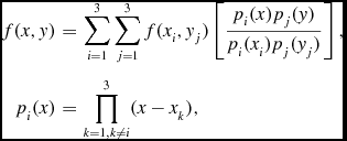
Because of the zone-level problem discussed in Section 3.7 it is only possible to determine T sys(η) in a piece-wise fashion within each HIPASS zone, each with an arbitrary zero point. The approach taken here side-steps these zonal discontinuities by measuring the derivative, dT sys/dη, and integrating. The constant of integration is chosen arbitrarily to set the minimum of T sys(η) to zero, which accords with our lack of knowledge of the zero level of the continuum emission over the sky as a whole.
The analysis was based on gridding using the observation that, in determining the gradient,
 \begin{equation}
\frac{T_n - T_1}{{\eta }_n - {\eta }_1} = {\sum _{i=2}^n \Delta {\eta }_i \Big(\frac{\Delta T_i}{\Delta {\eta }_i}\Big)} / {\sum _{i=2}^n \Delta {\eta }_i} ,
\end{equation}
\begin{equation}
\frac{T_n - T_1}{{\eta }_n - {\eta }_1} = {\sum _{i=2}^n \Delta {\eta }_i \Big(\frac{\Delta T_i}{\Delta {\eta }_i}\Big)} / {\sum _{i=2}^n \Delta {\eta }_i} ,
\end{equation}
The procedure then was to search for a dependence of T sys as a function of η and any other likely parameters, where η is the elevation of each separate beam. There was no dependence on azimuth, nor any discernible dependence on polarisation. However, there was a small but significant dependence on the zenithal position angle, ζ, which is defined as the angle between the zenith, the central beam (assumed to be positioned on the optical axis), and the beam in question. For the central beam, ζ is taken to be the rotation angle, ρ, of the feed assembly. Thus
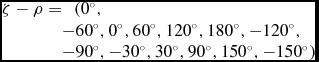 \begin{eqnarray}
\zeta - \rho = && ( 0\hbox{$^\circ $},\nonumber \\[-6pt]
&& \hspace*{-6pt}-60\hbox{$^\circ $}, 0\hbox{$^\circ $}, 60\hbox{$^\circ $}, 120\hbox{$^\circ $}, 180\hbox{$^\circ $}, -120\hbox{$^\circ $},\nonumber \\[-6pt]
&& \hspace*{-6pt}-90\hbox{$^\circ $}, -30\hbox{$^\circ $}, 30\hbox{$^\circ $}, 90\hbox{$^\circ $}, 150\hbox{$^\circ $}, -150\hbox{$^\circ $})
\end{eqnarray}
\begin{eqnarray}
\zeta - \rho = && ( 0\hbox{$^\circ $},\nonumber \\[-6pt]
&& \hspace*{-6pt}-60\hbox{$^\circ $}, 0\hbox{$^\circ $}, 60\hbox{$^\circ $}, 120\hbox{$^\circ $}, 180\hbox{$^\circ $}, -120\hbox{$^\circ $},\nonumber \\[-6pt]
&& \hspace*{-6pt}-90\hbox{$^\circ $}, -30\hbox{$^\circ $}, 30\hbox{$^\circ $}, 90\hbox{$^\circ $}, 150\hbox{$^\circ $}, -150\hbox{$^\circ $})
\end{eqnarray}
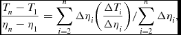
The general form of the dependence is
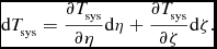 \begin{equation}
{\rm d}T_{\mathrm{sys}} = \frac{\partial T_{\mathrm{sys}}}{\partial \eta } {\rm d}\eta + \frac{\partial T_{\mathrm{sys}}}{\partial \zeta } {\rm d}\zeta .
\end{equation}
\begin{equation}
{\rm d}T_{\mathrm{sys}} = \frac{\partial T_{\mathrm{sys}}}{\partial \eta } {\rm d}\eta + \frac{\partial T_{\mathrm{sys}}}{\partial \zeta } {\rm d}\zeta .
\end{equation}
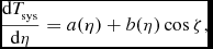 \begin{equation}
\frac{{\rm d}T_{\mathrm{sys}}}{{\rm d}\eta } = a(\eta ) + b(\eta ) \cos \zeta ,
\end{equation}
\begin{equation}
\frac{{\rm d}T_{\mathrm{sys}}}{{\rm d}\eta } = a(\eta ) + b(\eta ) \cos \zeta ,
\end{equation}
As described, the analysis is based on weighted median gridding of ΔTi /Δη i as a function of η and ζ by virtue of Equation (6). Because there are no parameters in Equation (9) that need to be determined as a function of ζ, it was possible to make the ζ grid much coarser than that of η in order to reduce the noise. Because η and ζ are true angles (not a spherical coordinate pair), the most appropriate choice of projection was a plate carréeFootnote 7 with the distanceFootnote 8 computed as
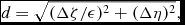 \begin{equation}
d = \sqrt{(\Delta \zeta /\epsilon )^2 + (\Delta \eta )^2},
\end{equation}
\begin{equation}
d = \sqrt{(\Delta \zeta /\epsilon )^2 + (\Delta \eta )^2},
\end{equation}
Noting that the convolution of a cosine function with a top-hat function produces a cosine of the same period but diminished amplitude, we would expect that such heavy smoothing of cos ζ should lead b(η) to be underestimated by 17%. However, smoothing was necessary to obtain reasonable statistics for each beam, especially when studied in isolation from the others, and particularly at higher elevations where the data is relatively sparse. This effect, and possibly others, were corrected by iterating the solution. Its magnitude was of the expected size.
At 5° × 15′, the (ζ, η) grid depicted in Figure 6 is considerably finer than the dimensions of the gridding kernel. As rotation of the feed assembly was limited to ρ = ±60°, ζ for each beam spans up to 120° or a third of the full range according to Equation (7). The portion of Figure 6 occupied by each beam was found to reproduce the behaviour established by gridding all beams together as in Figure 6.

Figure 6. dT sys/dη as a function of ζ and η for all beams taken together, obtained by weighted median gridding of ΔTi /Δη i .
Individually, Beams 2–7 in the inner ring were found to be indistinguishable, within the noise, from all of them taken collectively. Likewise for the outer ring. Also, a(η) for Beam 1 by itself did not differ significantly from the inner ring, though we set b(η) = 0 for it by consideration of symmetry. There were small but significant differences in a(η) for the inner and outer beams, as became clear when one was plotted against the other. However, b(η) for the inner and outer rings was found to be sufficiently similar within the noise, that they were taken to differ only by a scale factor. Consequently, there were three functions of η and two scale factors to be determined by least-squares fits to Equation (9). These were obtained from maps similar to Figure 6 but produced for Beams 2–7 only, and for Beams 8–13 only.
After integration, T sys is shown in Figure 7 as a function of η for values of ζ that define the envelope. For ζ = ±90°, T sys is set to zero at its minimum, whereas for other values of ζ it may dip slightly below zero in the vicinity. Clearly the effect of the b(η)cos ζ term in Equation (9) is significant, especially for η > 58°. The difference between the inner and outer beams is subtle yet important for accurate calibration when it is considered that this correction is added directly to the data. Accuracy is much reduced above η = 80° because there is little HIPASS/ZOA data in this regime but, by the same token, what little data there is to correct has a small impact on the final map. These curves are qualitatively similar to the curve (their Figure 4) measured by Griffith & Wright (Reference Griffith and Wright1993) for the PMN survey, which used the NRAO 7-beam system at 4850 MHz.

Figure 7. T sys as a function of elevation, η, for Beams 1–7 (left) and Beams 8–13 (right). The black curve at left applies for Beam 1, independent of ζ. Envelope curves are shown for beams in the inner and outer rings with ζ = 0° (dark grey), ± 90° (black), and 180° (light grey). The dotted curve in each is the nominal contribution from atmospheric opacity, T atm(1 − exp (−τ/sin η)), normalised at the zenith, using canonical values of T atm = 275 K and τ = 0.01.
An option was added to livedata to apply the T sys elevation correction on the fly when processing the data.
3.7 Zone-level adjustment
Figure 8 illustrates the final step to be overcome in producing the full continuum map, that of repairing the discontinuities at the declination zone boundaries, a process referred to here as zipping. The main handle that we have on this is the overlap between these zones. In principle it is clear that an offset can be computed by gridding the overlapping strips separately and differencing them. In practice, however, the overlaps are narrow and it is by no means clear that the results will be accurate enough, especially considering that errors will propagate from each overlap to every successive zone when the levels are computed. These form what are referred to below as streamers such as manifest themselves as the vertical artefacts in Figure 9.


Figure 9. HIPASS zone levels derived from the overlaps, before correction provided by ZOA. Particularly strong streamers emanate from the inner Galactic region (left). In general, streamers can be negative as well as positive. Plate carrée equatorial projection, 5401×15 pixels. Linear greyscale from −1 to +1 Jy beam−1, emphasising streamers.
The main source of streamers are strong compact continuum sources in the Galactic plane and this is where the ZOA survey comes to the fore. Because scanning in the ZOA survey was done in Galactic longitude, which for the range under study is always at an angle to the HIPASS scans in declination, the ZOA scans provide a bridge across the HIPASS declination zones in the region where the worst streamers are produced.
However, the ZOA zones (hereafter zoans to distinguish them from HIPASS zones) themselves require levels, so we are faced with a bootstrapping process. In summary, the HIPASS levels are first deduced as accurately as possible from the zone overlaps. These levels are then used to derive the ZOA zoan levels, which, once applied to the ZOA maps, are used to correct the HIPASS zone levels, particularly to remove streamers.
Thus firstly we must consider the HIPASS zone overlaps. Numerically, 81 000 levels had to be determined, one every 16 s of RA in 15 zones, though these values are not independent. Allowing one per 14.4 arcmin HPBW, the number of independent values would be about 14 800. However, considering that zone levels arise from emission that is significantly extended with respect to the 8° scan length, the true number is considerably less than this by perhaps a factor of eight or more, leading to a number less than 2 000.
3.7.1 HIPASS declination zone overlaps
Except for the two circumpolar zones, the HIPASS declination zones were stepped by 8° (=480 arcmin), i.e. ( − 87°, −82°, −74°, −66°, . . ., +14°, +22°). Typically the scans are 100×5 s integrations at 1 arcmin s−1, (500 arcmin) so naïvely we might expect a 10 arcmin overlap at each end. However, as seen in Figure 3, the inner beams contribute another 29 arcmin, and the outer beams another 51 arcmin at each end of the scan. Consequently, the usable overlap between zones is more like 45 arcmin.
However, at 1°.5, the overlap between the − 87° and − 82° zones is twice as wide, the data is also more uniformly distributed in this region of the sky because of grid convergence effects (see Figure 3), and there happens not to be any significant sources of emission to upset the measurements. Consequently, the offsets between these two zones are better determined than elsewhere and are considered not to require correction.
If the − 87° zone had extended to the SCP, or preferably slightly beyond it, then the southern edge of the zone would effectively have overlapped itself, and it would have been possible to set offsets for the zone by reference to the common point, the SCP, in each scan. However, as the Parkes telescope is based on a master equatorial drive system, the dish cannot scan through the SCP and necessarily stopped a short distance from it. Consequently, offsets for the − 87° zone were set by averaging integrations in the three map rows 8 arcmin, 12 arcmin, and 16 arcmin north of the SCP. Small offsets of up to 57 mJy beam−1 were required to achieve uniformity in this narrow strip.
In the first instance, the procedure was to map the overlapping strips separately using weighted median gridding onto a plate carrée projection of size 5401×11 pixels (or ×23 for the southern zones) spaced by 16 s in RA (4 cos δ arcmin) and 4 arcmin in declination. Iterative gridding was not used because adverse edge effects would have affected too high a proportion of each map. Instead the whole process was iterated as described later.
Overlapping strips were subtracted to produce a difference map, e.g. the northern strip of zone − 34° minus the southern strip of zone − 26°, which ideally should have constant brightness in declination. In practice, such constancy usually was observed to a remarkable degree, but in certain locations, particularly where the strip crossed the Galactic plane, there might be significant departures. Often this could be traced to a strong compact source that did not cancel exactly between the two strips; although it may have been a small fraction of the source strength, the residual would still be unacceptably high in absolute terms. This resulted in the streamers that will be discussed later. The zone offsets were computed by averaging the 11 (or 23) pixels across the width of the strip, potentially with censoring of such outliers.
With as few as 11 measurements, it was important to use the data as efficiently as possible. Offsets were computed for each RA as the median of the difference between the zone overlaps, southern minus northern. To improve statistics, $\lfloor 5 \sec \delta _{\mathrm{z}} \rfloor$
image columns spanning approximately 20 arcmin were aggregated, where δz is the mid-zone declination. However, as these samples are not independent, the improvement is somewhat less than it would otherwise be.
$\lfloor 5 \sec \delta _{\mathrm{z}} \rfloor$
image columns spanning approximately 20 arcmin were aggregated, where δz is the mid-zone declination. However, as these samples are not independent, the improvement is somewhat less than it would otherwise be.
The offsets were then subtracted from the difference map leaving a residual map in which outliers could clearly be identified. These tended to cluster near the southern or northern edges, or in localised areas of strong emission that failed to cancel exactly between the two zones. Sn computed for the residual map as a whole was used to censor these outliers. Starting from the SCP, the values obtained for Sn in each zone were: 15, 24, 27, 29, 40, 36, 35, 35, 37, 38, 41, 41, 41, 45, and 48 mJy beam−1. Only 0.27% of normally distributed data are expected to lie outside the 3σ confidence interval. However, averaging over all zones, 3.7% were found to lie outside 3×Sn , indicating the degree of departure from normality. Because one discrepant edge pixel could reasonably be expected in a scan of length 11 pixels, the offset was recomputed if up to 10% of the data was outside 3×Sn . Of the 81 000 offsets being determined, 60% were computed from data that had no outliers, and 29% were recomputed with a small number of outliers censored. The remaining 11% were not recomputed on the grounds that the value of Sn for the whole scan probably was not applicable to them and there was no way to improve on the median value.
The process of determining the offsets was iterated, with the offsets determined on one pass used for zipping the overlap strips on the next. The offsets provide everything required here and were used in preference to the levels to avoid complications that might arise from the accumulation of error in computing the latter. Iteration results in a small relative change because the offsets computed from the gridded maps are necessarily a smoothed version of the offsets that must be applied to the ungridded data. In practice, however, it mainly only served to demonstrate self-consistency. The offsets obtained are referred to as the core set to which reference is always made in subsequent processing.
3.7.2 Computing the HIPASS levels
The level for each of 5 400 RAs in each of the 15 declination zones was then computed by summing the core offsets from zone − 87°.
Negative levels of up to −133 mJy beam−1 then resulted in zone − 82° over an extended range of right ascension. These could not be attributed to noise alone, especially when, as previously explained, the offsets between these two zones are better determined than elsewhere. Also, there is no reason to suppose that the minimum in the continuum emission occurs at the SCP or anywhere near it. Consequently, the offsets in zone − 87° were adjusted upwards uniformly by 133 mJy beam−1, which has the effect of increasing all levels uniformly.
The levels were then smoothed lightly using a Gaussian of FWHM $4 \sec \delta _{\mathrm{z}}$
image columns, or approximately 16 arcmin. Considering that zone levels arise from emission that is significantly extended with respect to the 8°.5 scan length, much heavier smoothing in RA would be justified on the basis that there are no long, narrow sources of continuum emission that are oriented north–south on the sky. However, that was unnecessary and probably would have been counterproductive at this stage.
$4 \sec \delta _{\mathrm{z}}$
image columns, or approximately 16 arcmin. Considering that zone levels arise from emission that is significantly extended with respect to the 8°.5 scan length, much heavier smoothing in RA would be justified on the basis that there are no long, narrow sources of continuum emission that are oriented north–south on the sky. However, that was unnecessary and probably would have been counterproductive at this stage.
Determination of the zone levels by integrating the offsets amounts to a simple one-dimensional random walk, the variance of the level at any point being equal to the sum of the variances of the steps preceding it. Noting that the values of Sn
computed for each zone above were for the dispersion of the data used to compute the offsets, the equivalent of the standard error in the mean should be obtained by dividing by $\sqrt{n}$
. However, we have used the median, which is less efficient than the mean, but on the other hand, aggregated image columns spanning 20 arcmin, though they did not provide independent samples. Taking the overlap width divided by the HPBW, n = 3 (or 6), as a lower limit for n, and omitting the − 87° zone, which defines an arbitrary zero level, the 1σ uncertainty in the levels in each zone should be less than 0, 10, 18, 25, 34, 40, 45, 49, 53, 58, 62, 67, 71, 75, and 80 mJy beam−1. These provide target figures for the potential accuracy of the zipping operation. However, as indicated previously, Sn
is abnormally high for about 11% of the measured offsets, mainly for those scans that traversed the Galactic plane. Thus the uncertainty in the levels computed from these offsets can be much higher and this is what gives rise to streamers.
$\sqrt{n}$
. However, we have used the median, which is less efficient than the mean, but on the other hand, aggregated image columns spanning 20 arcmin, though they did not provide independent samples. Taking the overlap width divided by the HPBW, n = 3 (or 6), as a lower limit for n, and omitting the − 87° zone, which defines an arbitrary zero level, the 1σ uncertainty in the levels in each zone should be less than 0, 10, 18, 25, 34, 40, 45, 49, 53, 58, 62, 67, 71, 75, and 80 mJy beam−1. These provide target figures for the potential accuracy of the zipping operation. However, as indicated previously, Sn
is abnormally high for about 11% of the measured offsets, mainly for those scans that traversed the Galactic plane. Thus the uncertainty in the levels computed from these offsets can be much higher and this is what gives rise to streamers.
The zone levels obtained are shown in Figure 9 with obvious streamers extending northwards from the Galactic plane, particularly in the vicinity of the Galactic centre. The result of applying them when gridding may be seen in Figure 11a. This is essentially what would be obtained by adding Figure 9 to Figure 8 (on the same projection), the zone-level correction being additive. Streamers are clearly evident. The next step is to refine these levels by crossing HIPASS with ZOA.
3.7.3 Crossing HIPASS and ZOA: (a) computing the ZOA levels
After bandpass calibration, ZOA scans have an arbitrary offset just as do the HIPASS scans. The first step in improving the HIPASS zone levels is to derive these ZOA zoan levels. Figure 10 illustrates that process graphically. Of course, the zoan levels are also needed so that the large ZOA data set can be included in the final map, substantially reducing the noise in the interesting Galactic plane region.
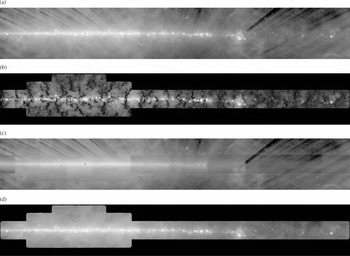
Figure 10. Graphical depiction of the first iteration of ZOA zoan-level determination based on HIPASS. In each case, the data are gridded onto a plate carrée projection in Galactic coordinates, + 53° ⩾ ℓ ⩾ −165°, |b| ⩽ 16°. The inputs are (a) HIPASS zipped using levels deduced from the declination zone overlaps, and (b) ZOA without levels, analogous to Figure 8. The difference between these, (c), is used to derive the levels for ZOA, which when applied yield (d). In practice this is done separately for each ZOA zoan, with the levels derived by averaging in Galactic longitude. Logarithmic greyscale as for previous figures.
For each ZOA zoan, zone-adjusted HIPASS data were gridded onto a plate carrée projection in Galactic coordinates, dimensioned so that it just covered the zoan. ZOA data was also gridded onto an identical projection. The image width, which is the critical dimension, was 129 pixels spaced by 4 arcmin. The difference between these two maps, HIPASS minus ZOA, should be constant in Galactic longitude, though varying in Galactic latitude. This is the zoan level, i.e. the offset that was lost during bandpass calibration.
As in Section 3.7.1, iterative gridding (Section 3.3.1) was not used in order to avoid edge effects. However, the whole procedure was iterated as described in Section 3.7.5.
In practice, because of errors in the HIPASS zone levels, the difference maps are not quite constant in Galactic longitude, particularly in being affected by residual streamers, as seen in Figure 10c. However, as the streamers cross at an angle to the parallels of Galactic latitude, mostly they only affect a part of the scan in Galactic longitude from which the zoan level is determined.
Unlike the HIPASS levels, which must be derived by summing offsets, the ZOA levels are obtained directly. As for the HIPASS zone offsets, they are computed as the median value across the scan in the difference map (Figure 10c). In contrast to HIPASS, there is a full 8°.5 of overlap to work with, rather than 45 arcmin, and smoothing of the levels was not warranted. However, censoring of outliers was performed as before. That is, the zoan levels were subtracted from the difference map to produce a residual map. Pixels outside 3×Sn in this map were deemed to be outliers, where Sn was computed from the map as a whole, and the zoan levels then recomputed. Visual inspection showed that this was particularly effective at removing outliers associated with areas of strong emission that did not cancel due to small relative errors between the HIPASS and ZOA maps.
Figure 10d was produced from zoan-adjusted ZOA data, a remarkable development of the uncorrected map seen above it. It bears a close resemblance to the first-pass HIPASS map of the Galactic plane in Figure 10a, but much less affected by streamers. This suggests that it may be used for improving the HIPASS zone levels.
3.7.4 Crossing HIPASS and ZOA: (b) refining the HIPASS levels
Differencing Figures 10a and 10d produces a map, seen in Figure 12a, that consists mostly of residual artefacts—streamers—in the HIPASS map, together with strong sources that do not quite cancel. However, Galactic coordinates are not the best choice because the streamers are oriented at different angles depending on Galactic longitude. In equatorial coordinates on a cylindrical projection the residual streamers all run north–south, as seen in Figure 11a. When the zoan-corrected ZOA data is gridded onto an identical projection, and the difference taken, the residual streamers manifest themselves as vertical stripes as seen in Figure 11c, and as such are amenable to measurement and subsequent correction.
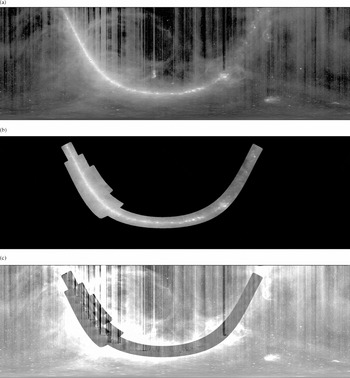
Figure 11. Graphical depiction of the first iteration of HIPASS zone-level correction based on ZOA. In each case, the data are gridded onto a plate carrée projection but this time in equatorial coordinates, 24h ≥ α ≥ 0h, − 90° ⩽ δ ⩽ +26°. The inputs are (a) HIPASS zipped using levels deduced from the declination zone overlaps, as per Figure 10a, and (b) ZOA with levels deduced as per Figure 10d. The difference between these, (c), is used to derive level corrections for HIPASS. In practice this is done separately for each HIPASS zone, with the correction derived by averaging in declination. Logarithmic greyscale as for previous figures except for (c), which is a linear scale from −1 to +1 Jy beam−1.
The procedure was similar to the forgoing. Maps on a plate carrée projection, this time in equatorial coordinates, were produced separately from HIPASS and ZOA data for each HIPASS zone that intersects the ZOA, namely − 66° and northwards. These are long thin strips, 5401×161 pixels, of which the ZOA data only fills a portion. A correction to the levels was obtained as the median value across the scan in declination, with censoring of outliers applied as before. Again, visual inspection confirmed the validity of the censoring. A correction was computed if, after censoring, at least five pixels remained in the declination strip.
At this point we have a set of corrections to the zone levels. In fact, what is required is a correction to the core set of offsets that were derived in Section 3.7.1. Whilst there was only one place to apply the 133 mJy beam−1 offset introduced to ensure non-negativity in zone − 82°, namely in the zone − 87° offsets (Section 3.7.2), for more northerly zones the residual could be applied to any of the zones further south. In practice, levels were adjusted by distributing the residual amongst the offsets in zones south of the level being corrected on a pro-rata basis according to the variance (S 2 n ), excluding zones − 87° and − 82°. This tended to place almost all of the correction in the Galactic plane.
This process provided corrections to 13.8% of the HIPASS levels. Wherever no correction was obtained from ZOA, the offsets were replaced with the corresponding offset from the core set. In particular this included all offsets to the east, north, and west of the ZOA survey area.
3.7.5 Crossing HIPASS and ZOA: (c) iteration and convergence
After refining the HIPASS levels it seems obvious that they could be used to produce a better estimate of the ZOA levels. Accordingly, the procedure described in Section 3.7.3 was repeated. In turn, the new estimate of the ZOA levels could then be used to improve the HIPASS levels. In effect such an iterative process exploits the fact that HIPASS scans may form a bridge between adjacent ZOA zoans from which the relative zoan levels can be determined. Likewise, the ZOA scans may form a bridge between adjacent HIPASS scans. However, unlike the HIPASS zone overlaps where the overlapping scans are parallel to each other, these bridges cross at an angle. Thus, instead of providing the offset between a pair of scans on opposite sides of a discontinuity, they provide the offset between sets of scans on either side. Complicated as the geometry may be, it seems reasonable to expect that convergence should be obtainable. That is, we expect that there is a set of HIPASS and ZOA levels for which the difference between the HIPASS and ZOA maps is zero plus noise, and we anticipate that iteration will find them. However, there are complications.
In successive iterations, as the HIPASS levels are expected to be better determined, the streamers should reduce in size and generally have less of an effect on the determination of the ZOA levels. Indeed, very few streamers survived even a single iteration. However, it was found that if the streamers were wide enough on the first pass, and the angle acute enough, then they could cause the iteration to fail to converge over part of the map. The problem is evident in sections of the ZOA north of the Galactic centre region in Figure 12.
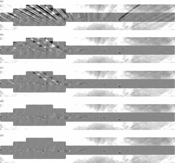
Figure 12. Progress of the iteration depicted graphically—HIPASS minus ZOA after (a) zero, (b) one, (c) two, (d) four, and (e) ten passes of refining the HIPASS levels. (Figure (a) is equivalent to Figure 11c.) Most of the narrow streamers have disappeared after a single pass leaving only intransigents that emanate from the Galactic centre region. These are slowly eaten away in subsequent passes. The subtle saw-tooth residual, which appears below the Galactic centre region, becomes more noticeable as the streamers are corrected, but is gone in the final pass with special handling. Same projection as Figure 10. Linear greyscale from −1 to +1 Jy beam−1.
The characteristic blocky structure seen in Figure 12b indicates that wide streamers have corrupted the zoan levels over a range of Galactic latitude in adjacent zoans. In fact, this can be seen directly in Figure 10d, whilst close inspection of Figure 12b reveals that all zoans between 344° and 48° were affected to some degree. These intransigents persist through successive passes, indicating that they form part of a stable, yet clearly incorrect solution of the iteration. The cure, applied in the second and third passes, was simply to identify and excise the affect ranges of Galactic latitude in each zoan of the ZOA maps from the next pass of the iteration. The bad latitudes are those associated with the dark blocks in Figure 12b. The bright corners are so because they correctly identify the positive excess due to the positive streamer (in this case). Effectively these bright corners eat into the streamer on the next pass, eliminating the smaller intransigents, and reducing the width of the larger ones in Figure 12c. After four passes the intransigents have been completely eaten away in Figure 12d.
The HIPASS maps produced in each pass always applied the best estimate of the levels available, namely those obtained from the previous pass. Thus subsequent iterations only provided corrections to the levels from the previous pass. As mentioned in Section 3.7.1, iterating corrects for the subtle effect that the levels computed from the gridded maps are necessarily a smoothed version of the levels that must be applied to the ungridded data. However, until the intransigent streamers had been completely removed, the ZOA maps used to compute the zoan levels (Section 3.7.3) were all produced without levels. That is, the uncorrected map shown in Figure 10b was used each time. This provided a fixed reference point from which the convergence behaviour could be assessed. The remaining iterations were then done with zoan levels applied.
As the difference between the HIPASS and ZOA maps should consist solely of noise together with a few outliers associated with strong sources, Figure 12 shows that, when present, the effect of streamers or other defects is readily apparent on visual inspection. Thus the convergence behaviour could be monitored qualitatively at a glance. After dealing with the intransigent streamers, a new type of artefact assumed prominence albeit at a lower level. It appears in Figure 12d below the Galactic centre region as a saw-tooth pattern with an amplitude of about 100 mJy beam−1. This pattern arises from a different mechanism to the intransigent streamers and disappears slowly in successive iterations. However, after eight passes it was apparent that the convergence was slow enough to warrant investigation of a more direct solution.
Thus far we have not considered the overlap between adjacent ZOA zoans. Although they offer an independent mechanism for tying together the ZOA zoans, and hence the HIPASS zones, these overlaps are problematic for two reasons. Firstly, unlike HIPASS where the scans all converge on the SCP, ZOA scans when tied together have no common point so there is no way to relate scans in neighbouring Galactic latitudes. Secondly, strong sources within a degree or two of the Galactic plane render the determination of offsets very uncertain, with the formation of prominent streamers in Galactic longitude akin to those in declination in the HIPASS levels. However, on further investigation it was apparent that the saw-tooth pattern was generated by steps in the levels between adjacent zoans. Only one value is needed per zoan to eliminate the pattern, and there is sufficient information in the ZOA overlaps to measure these steps directly.
Although a faint pattern is also visible in the Galactic anti-centre region, it seemed best to allow iteration to deal with that naturally. Thus we focus on the Galactic bulge region, measuring the offsets for each latitude only in the extensions where |b| > 6°, well away from bright sources in the plane. These measurements were averaged into one single offset for each pair of zoans from 336° to 32°. The offsets were then converted to zoan-level corrections as in Section 3.7.2, and renormalised to zero for zoan 336° and the zoans preceding it. Corrections for the 48° and 40° zoans were set equal to that for the 32° zoan. Thus only seven independent corrections for the ZOA zoan levels were computed, amounting to 300 mJy beam−1 from zoan 336° to zoan 32°. Once applied, the saw-tooth disappeared quickly; on the next iteration the difference in the levels had dropped by a factor of ×15, with a further factor of ×3 in the iteration after that, reducing it to a negligible value.
Iteration continued until there was no substantive change in the difference maps shown in Figure 12. Convergence was considered to have been achieved after ten passes of refining the HIPASS levels and one further round of computing the ZOA levels from them. Bright source ghosts form the most prominent residual artefacts visible in Figure 12e. These are expected as previously explained. Fine-scale HIPASS streamer noise, the leftovers of imperfect streamer removal, can be detected over most of the difference map. Away from the Galactic centre it has a peak height of about 50 mJy beam−1, but may become more prominent where it crosses bright extended sources. There is no evidence of any residual from the ZOA levels.
HIPASS zone boundaries are also visible in the difference map in the Galactic centre region, mostly a positive excess of up to 100 mJy beam−1 but systematically going negative where the boundary crosses the plane. This behaviour seems to be confined to regions of very strong extended emission. It was not removed by iterative gridding and currently its cause is not understood. Again, following treatment of the saw-tooth residual, there is almost no evidence of the ZOA zoan boundaries. In areas well away from residual artefacts the rms of the difference map is 20 mJy beam−1. Assigning the relative contribution to this from HIPASS and ZOA in the ratio $\sqrt{5}:1$
, the rms of the component maps would be 18 mJy beam−1 and 8 mJy beam−1 as best case noise figures.
$\sqrt{5}:1$
, the rms of the component maps would be 18 mJy beam−1 and 8 mJy beam−1 as best case noise figures.
As previously explained, the error in the levels determined from the HIPASS zone overlaps in Section 3.7.2 is expected to be highest in the + 22° zone, and this was confirmed, with corrections in the range ±1.5 Jy beam−1, an rms of 320 mJy beam−1, and a mean value consistent with zero.
Figure 13 presents the uncorrected HIPASS levels obtained from the declination zone overlaps together with those resulting from ten passes of crossing HIPASS and ZOA. The worst of the streamers originating in the Galactic plane have disappeared from Figure 13b, but some prominent streamers remain, clearly originating from strong extra-Galactic continuum sources, notably Cen A. The final step is to fix these individually and then smooth the levels.

Figure 13. HIPASS levels (a) before correction (same as Figure 9), (b) after correction by crossing with ZOA, and (c) the final result after conditioning. Strong Galactic streamers have all disappeared in (b) leaving the prominent Cen A streamer visible just left of centre, together with low-level streamer noise. Same projection and linear greyscale as Figure 9.
3.7.6 Conditioning the HIPASS levels
Figure 13b shows the HIPASS levels obtained after correction by crossing HIPASS and ZOA. Residual streamer noise is visible with peaks to about 100 mJy beam−1, though with several stronger. The source of five of these was readily identified, including Cen A, and it was verified that the offset computed from the relevant HIPASS zone overlaps in Section 3.7.2 had a high value of Sn due to these sources. As they lie outside the ZOA survey, none of them were amenable to correction by the previous methods. However, as these streamers have an obvious source, it was straightforward to apply an offset that would make them disappear into the background streamer noise. For Cen A this required an adjustment of −550 mJy beam−1 (Gaussian peak) over 19 levels (FWHM) spaced by 16 s in RA; for 3C273, +300 mJy beam−1 over 9 levels; for 30 Doradus with two separate streamers, +200 mJy beam−1 and +140 mJy beam−1 both over 10 levels; for PKS J1935-4620, −300 mJy beam−1 over 12 levels; and for PKS J0303-6211, +130 mJy beam−1 over 10 levels. The correction was applied entirely to the offset between the zone containing the source and its neighbour to the north.
After dealing with these outliers, the remaining streamers appear to have a noise-like distribution, with as many positive as negative and no obvious correlation between them. As explained previously, the process of computing HIPASS levels amounts to a simple one-dimensional random walk for which the variance at any point is equal to the sum of the variances of all steps leading to it. Hence the streamer noise is expected to be lower in the south and higher in the north, as is observed qualitatively. Indeed, all of the processing to this point has carefully treated positive and negative streamers equally so as not to introduce biasses that might disturb this random distribution.
The final step then was to smooth the levels in right ascension. Previous processing only used very light smoothing, but considering that zone levels arise from emission that is significantly extended with respect to the 8°.5 scan length, much heavier smoothing in RA is justified on the basis that there are no long, narrow sources of continuum emission that are oriented north–south on the sky. Bear in mind that only the levels are smoothed, not the final map. The question then arises of the maximum valid smoothing length, and what length is sufficient to remove the streamers.
The ZOA levels were used for guidance in assessing a legitimate smoothing length. The strong peak that occurs right on the Galactic plane was found to be the only narrow feature. The zoan levels on either side of it change gradually, with only a few, relatively weak features with a scale length in the range from 1° to 2°. It was also apparent that the ZOA levels are well determined and do not require smoothing. Considering that the HIPASS sampling rate is overwhelmed by a factor of ×5 in the region of the ZOA survey, the choice of smoothing length for the HIPASS levels is not a significant concern in this region. Moreover, in light of the results of Section 3.7 in using ZOA to eliminate HIPASS streamers, smoothing of the HIPASS levels within the ZOA survey area should be kept to a minimum. In practice it was only done to prevent discontinuities on the boundary of the survey.
Several smoothing strategies were investigated, the simplest being to smooth the levels in right ascension. In fact, this is the least effective method because it does nothing to stop streamer formation. By smoothing the offsets, streamers are attenuated close to their source, before they can propagate northwards. However, unless the ZOA region is smoothed identically, offsets do not balance between zones northwards of the Galactic plane, leading to the formation of streamers. Thus the most effective smoothing method was found to be a combination of the two approaches. Starting from the south, the levels for one zone are smoothed, then the levels for the next zone (outside the ZOA) are recomputed from these smoothed levels and the original offsets. The next zone is then smoothed in turn. This strategy attacks streamers at their source, and also has the benefit of smoothing a quantity that will appear directly as emission on the final map.
In practice an empirical approach was used to determine the smoothing length. Essentially the levels were put through a high-pass Gaussian filter and the smoothing length adjusted to best effect, giving little weight to the ZOA survey area. Starting with a short smoothing length, only streamer-like noise made it through the filter—long filaments oriented north–south with no obvious structure that could be related to any celestial emission. As the smoothing length was increased, shorter and wider features appeared that could be related to genuine cosmic emission. A length of 4° FWHM was found to be the best compromise for streamer removal and retention of genuine emission in regions outside the ZOA. The rms of the high frequency streamer components was about 100 mJy beam−1 in the + 22° zone being the worst case. Having determined the appropriate filter length, the levels were then smoothed using a low-pass Gaussian filter of the same filter length. Within the ZOA, a length of 1° was sufficient to avoid discontinuities at the edges of the survey area.
As can be appreciated from Figure 11, the ZOA overlaps the HIPASS scans to a variable extent. Some HIPASS scans and their neighbours have the benefit of a complete intersection, whilst others intersect only partially. In particular, only a small corner of the 200° and 48° ZOA zoans intersect the + 22° HIPASS zone, with the 48° corner proving troublesome. As stated in Section 3.7.4, a correction was computed if, after censoring, at least five pixels remained in the overlap. However, compared with peak values of around 130 pixels, corrections based on such a small number of pixels cannot be said to be fully within the ZOA survey area, nor be treated with the same degree of confidence. Thus, in order to prevent discontinuities on the boundary of the ZOA survey and to clean up nuisance streamers generated in the boundary regions, it was found necessary to use a graduated definition of inclusion. A level was considered to be fully inside the ZOA if the correction was computed from a certain minimum number of pixels, n 0, and fully outside if there was no correction (in practice, less than five). Progressive smoothing operated within the margins, with the FWHM of the smoothing length varied pro rata between 1° (inside) and 4° (outside) according to the number of pixels used to compute the correction. Noting the gradual effect that changing n 0 had on the results, a value of n 0 = 50 pixels was determined empirically.
The final HIPASS levels are shown in Figure 13c. At this stage the levels ranged from −0.34 to +9.1 Jy beam−1.
3.8 Final steps
The final map was produced by iterative gridding using a single iteration and a loop gain of 1.2, as discussed in Section 3.3.1. As mentioned in Section 3.1, some sources were strong enough to saturate the receiver power detection system, including several bright HII regions in the Galactic plane. This was more apparent in the relative sensitivity map (Figure 16) than in the brightness map itself. The pixel value in the sensitivity map is the square root of the sum of squares of the beam weights used in producing the brightness map. A value of n is essentially equal to n 2 independent boresight observations. Pixels at, or in the neighbourhood of saturated peaks appeared as shadows in the sensitivity map. The brightness computed for these pixels would be affected by the absence or asymmetric distribution of data, though with regard to the latter it should be noted that iterative gridding does tend to correct for this naturally. Steps were taken to repair these areas of the map as far as possible, and to blank any remaining unreliable pixels.
3.8.1 Blanking unreliable pixels
As can be seen in Figure 3, the reliability of pixels north of δ = +25° reduces as the density of the data gradually diminishes. These pixels were blanked by imposing a cut-off in the value of the relative sensitivity over the whole of the brightness map. A value of 4.0 units was found to be an effective level. On this basis the northern boundary of the map has been allowed to remain ragged. This filter also blanked eight pixels at the SCP, and 60 pixels known to be associated with saturated sources.
As explained in Section 3.1, data flagged by the multibeam correlator were properly handled in this analysis. Pixels affected by flagging were found by producing a map representing the proportion of flagged data that would have (but did not) contribute to each pixel in the brightness map, this type of map being more effective at highlighting the influence of flagged data than the sensitivity map. Apart from source saturation, data might also be flagged because of strong RFI, and its effect was certainly evident in this map. However, the criterion set to exclude obviously saturated pixels also reliably ignored all RFI-affected pixels. Thus, 256 pixels (0.004% of non-blank pixels) were found where more than 15% of the data was flagged. These pixels convincingly matched all of the bright sources suspected of being saturated.
Next, new maps were produced as before, but this time with a 5 arcmin cut-off radius for the gridding kernel instead of 6 arcmin. The density of data in the Galactic plane (ZOA) region may be high enough even with a 2 arcmin radius to be above the relative sensitivity cut-off of 4.0 units. Reducing the cut-off radius should exclude flagged data for pixels on the periphery of strong sources, and indeed 6 of the 256 pixels were reclaimed. Matching pixels in the sensitivity map were updated with the reduced value from the smaller gridding kernel. The radius was further reduced to 4 arcmin, 3 arcmin, and then 2 arcmin with the reclamation of a modest 2, 3, and 5 pixels respectively. Inevitably, a remainder of 240 pixels (additional to the original 60) were too close to strong peaks to be recoverable. These were blanked and the matching pixels in the sensitivity map were zeroed. Saturated sources and the associated number of blanked pixels are identified in Table 3.
Table 3. A total of 300 pixels were blanked from the following 16 saturated sources.
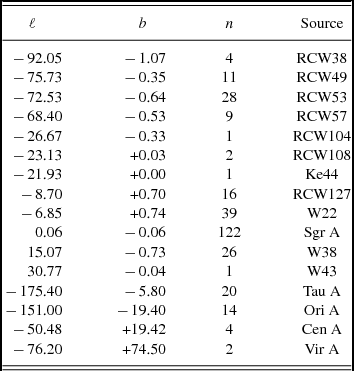
3.8.2 Brightness calibration
The raw HIPASS data is calibrated reasonably accurately for flux density; all brightness values quoted so far are with respect to this nominal scale. The calibration was checked via Gaussian fits to the peak height of two sources in the compact source map (Figure 1): 1934-638 (14.9 Jy), and Hydra A (40.6 Jy). The mean of the calibration factors (1.11, 1.07) was 1.09.
The final steps required to obtain a fully calibrated flux density image are: (a) to determine and apply a zero level; and (b) to apply the overall flux density scale. Non-negativity required a global offset of +310 mJy beam−1, with the minimum occurring on the northern edge of the north polar spur, close to the NGP. The above scale factor of ×1.09 was then applied.
The final map prior to scaling is presented in Figure 15 for comparison with the previous maps. It should be considered in conjunction with the relative sensitivity map of Figure 16.
Conversion to absolute brightness temperature depends on the unknown zero level and the Jy to K scale factor. The former can be measured using calibration horns; the latter ratio can be calculated if the beam has been accurately measured out to distant sidelobes. Fortunately, we can obtain both values by comparison with the lower resolution all-sky 1420 MHz mapFootnote 9 derived from the surveys of Reich (Reference Reich1982), Reich & Reich (Reference Reich and Reich1986), and Reich et al. (Reference Reich, Testori and Reich2001). This plate carrée map was regridded onto a Hammer-Aitoff projection, it being necessary to use an equiareal projection for the purpose. The present map was first regridded onto an equatorial plate carrée projection; then blurred to 35.4 arcmin resolution, first in RA with a 32.3 arcmin FWHM Gaussian kernel (the number of pixels therefore varying with declination) then in declination; and then regridded to match the other map. As the least-squares analysis of offset and scale was distorted by the preponderence of data below 5 K, the data was sorted into 10 mK bins. A factor of 0.44 K/(Jy beam−1) with offset 3.30 K was obtained and used to convert the final map to units of absolute brightness temperature.
The resulting cross-plot of some 470 000 pixels is shown in Figure 14 and shows excellent agreement. Like Haslam et al. (Reference Haslam, Salter, Stoffel and Wilson1982), the Reich et al. maps use a full-beam brightness temperature computed for a very extended beam of 7°. The brightness temperature scale for the Parkes map is therefore consistent with this. A conversion value of TB /S = 0.44 K/(Jy beam−1) also allows compact source fluxes to be measured accurately (though it is recommended to use the compact source map in Figure 1 for this purpose). Nevertheless, the implied main beam efficiency is only 51% with respect to a Gaussian beam with a HPBW of 14.4 arcmin. This is even lower than the quoted Stockert beam efficiency of 55% (Reich, Reference Reich1982). Values of TB /S = 0.80 K/(Jy beam−1) are typically used in HI observations of extended objects at Parkes, e.g. Staveley-Smith et al. (Reference Staveley-Smith, Kim, Calabretta, Haynes and Kesteven2003). Some of the lower efficiency is due to the use, in the present work, of all the off-axis beams, the outer of which is 26% less efficient than the central beam. As discussed in Barnes et al. (Reference Barnes2001), there are similar factors that arise from the nature of the gridding function and the subsequent variation of beam size with the angular scale of the source, some of which was absorbed in the previously discussed flux calibration factor of 1.09. Nevertheless, a conversion value closer to TB /S≈0.57 K/(Jy beam−1) might have been expected. It therefore remains possible that some of the ~30% residual difference is due to sidelobe power on intermediate scales ( < 7°). Structures on this scale may be slightly less prominent than they would be with a telescope with a pure Gaussian beam. However, the excellent match with the lower resolution data (Figure 14) after application of a single overall scale factor, implies high consistency with previous work in the field.
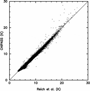
Figure 14. Cross-plot of the present HIPASS/ZOA map blurred to $35\hbox{$.\hspace{-2.22214pt}^\prime $}4$
resolution versus the 1420 MHz all-sky map of Reich et al. (Reference Reich, Testori and Reich2001).
$35\hbox{$.\hspace{-2.22214pt}^\prime $}4$
resolution versus the 1420 MHz all-sky map of Reich et al. (Reference Reich, Testori and Reich2001).
4 DISCUSSION
In this section, we discuss the reliability and calibration of the final map at various angular scales. In particular, during the course of data reduction, we have applied several important additive corrections. What is the cumulative effect of these?
Fortunately, the main effects we have corrected for manifest themselves prominently as image artefacts with a definite signature. The data can be re-ordered in various ways to accentuate these effects. Thus, the T sys elevation dependence, which has an obvious signature in Figure 2, is distilled for measurement in Figure 6. Judging from the scale of Figure 7, the maximum error across a scan is unlikely to exceed 100 mJy beam−1 in the worst case, which is at the SCP and the northern elevation limit. In fact, over most of the sky the effect tends to cancel due to the random orientations of the scans. Subtracting Figure 8 from Figure 2 revealed a correction of up to 1 Jy beam−1 along the northern perimeter and 650 mJy beam−1 in the vicinity of the SCP. At mid-latitudes there are isolated patches where the correction exceeds 100 mJy, but mostly it is below this. These are the absolute corrections, the error would be much less. If it was as much as 10% then the residuals would range from less than 10 mJy beam−1 (mostly) up to 100 mJy beam−1 depending on location (5 mK to 48 mK).
Similarly, errors in the determination of the HIPASS and ZOA levels manifest themselves as obvious artefacts—streamers—as seen in Figure 13. Most of the streamers were eliminated by smoothing the levels, the only obvious residuals being a short pair associated with Fornax A. Again the error is highly dependent on location in the map, with northern declinations the most affected as previously explained.
The most obvious artefacts remaining in the final image of Figure 15 resemble fine brushstrokes consistent with the pattern seen in Figure 3. Again, these are highly dependent on location, mostly occurring in isolated patches outside the ZOA at levels of up to 50 mJy beam−1 (22mK) at the worst, too low to warrant de jure smoothing of the whole map. However, sections of the map would certainly benefit from light smoothing at the discretion of the end user. There is no clear evidence in the final map of the HIPASS zones or ZOA zoans or the seams between them. However, these may become apparent on differencing with other surveys.
Figure 15. HIPASS and ZOA data combined to produce the final version of the 1.4 GHz ‘CHIPASS’ continuum map. This map has been rezeroed but not rescaled so as to be comparable with Figure 8, using the same logarithmic greyscale.
The cross-plot in Figure 14 of CHIPASS versus the 1420 MHz all-sky map derived from Reich (Reference Reich1982), Reich & Reich (Reference Reich and Reich1986), and Reich et al. (Reference Reich, Testori and Reich2001) demonstrates excellent agreement overall. Curiously, most of the worst outliers at high values, both above and below the line, arise from W51 and W44. As shown by the difference map in Figure 17, there is excellent agreement between the two maps for compact sources and structures up to about 60° in angular size, including the North Polar spur, the Gum nebula, Barnard’s Loop, and the many wispy tendrils that emanate from the plane of the Milky Way. Reassuringly, some structures at northerly declinations that looked at first sight as though they might be residuals from the T sys elevation correction and/or HIPASS zone-level correction do have counterparts in the Reich et al. map. The larger depression south of the plane indicates a discrepancy of up to 0.8 K from the mean. Likewise the more compact 1.2 K depression at the end of the plane and the dark streak leading to it. This area produces the small bulge below the line at low values in the cross-plot of Figure 14. The depression is visible in the 408—1420 MHz spectral index map shown in Reich, Reich, & Testori (Reference Reich, Reich, Testori, Uyaniker, Reich and Wielebinski2004) and was previously suspectedFootnote 10 to be an artefact caused by the large number of scans terminating at the Galactic plane, though with relatively small effect on the spectral index in this bright region of the sky.
CHIPASS produces barely discernible seams, about 20 mK in height, that delineate HIPASS zones south of δ = −58°. The CHIPASS zero level has been set close to that of Reich et al. with the mean difference in more settled areas away from the Galactic plane at about 0 K. The rms computed over sample areas of about 400 square degrees in settled regions varies from 15 mK to 60 mK depending strongly on location, with 40 mK being typical. This being a difference map, if shared equally, the error attributable to each map would be less by $\sqrt{2}$
. On this basis a typical rms error of 30 mK may be assigned to the CHIPASS map, excluding the error in the zero level. However, Figure 17 highlights areas where the rms may be much higher.
$\sqrt{2}$
. On this basis a typical rms error of 30 mK may be assigned to the CHIPASS map, excluding the error in the zero level. However, Figure 17 highlights areas where the rms may be much higher.
The rms of the CHIPASS minus Reich et al. difference map is more in the nature of an absolute error (on all spatial scales) rather than just noise. It is closely related to the scatter in the cross-plot of Figure 14, the main contribution to it undoubtedly being localised baseline error. It is not simply related to what would normally be quoted as the rms noise or sensitivity for surveys of this type.
Typically the intrinsic rms noise would be computed from the scatter in source-free regions of a map. That is impossible here because of the high source density, but a number can be obtained from the difference between the HIPASS and ZOA maps (as in Section 3.7.5). It is clear in Figure 12e that strong sources on the Galactic plane do not cancel exactly in the difference map, and that is readily understood to arise from small errors in the flux density calibration between the two, as well as effects that may arise in gridding irregularly sampled data. Looking in the very quietest regions of Figure 12e and choosing sample areas so as to exclude source residuals as much as possible, the smallest rms that can be measured over a few hundred pixels is 20 mJy beam−1, most of which must arise from the less-well sampled HIPASS map. Applying a correction of $\sqrt{5/6}$
for the noise contributed to the difference by the ZOA map brings this figure down to 18 mJy beam−1. That gives an rms of 8 mK for the HIPASS-only regions outside the ZOA and Sculptor deep field (Figure 16), and on this basis we have adopted a nominal figure of 40 mK, or 90 mJy beam−1 (being 5 × rms), for the sensitivity.
$\sqrt{5/6}$
for the noise contributed to the difference by the ZOA map brings this figure down to 18 mJy beam−1. That gives an rms of 8 mK for the HIPASS-only regions outside the ZOA and Sculptor deep field (Figure 16), and on this basis we have adopted a nominal figure of 40 mK, or 90 mJy beam−1 (being 5 × rms), for the sensitivity.
Figure 16. Sum in quadrature of the beam weights (BeamRSS) used in producing the final map, a measure of sensitivity. A value of n is essentially equal to n 2 independent boresight observations. A typical value for HIPASS outside the ZOA survey area is around 7, increasing to 9 in the zone overlaps and the RA = 0h/24h seam. Near the SCP and in the zone − 87°/ − 82° overlap it increases to 11, but note the pinhole right at the SCP itself. Deeper mapping was done in the SGP region, with values in the range 10–12, and up to 21 in the Sculptor deep field. Values range between 18 and 23 within the ZOA. Saturated sources may be identified as local depressions (when viewed at full resolution). Linear greyscale ranging from 0 to 23.
Carretti et al. (in preparation) kindly provided a pre-publication continuum map derived from S-PASS for comparison with CHIPASS. This southern hemisphere (δ < 0°) polarisation survey at 2.3 GHz was made with a single beam system on the Parkes radio telescope using a long-azimuth-scan, basketweaving observing strategy tailored for the purpose (Carretti, Reference Carretti, Kothes, Landecker and Willis2011). The S-PASS continuum map with HPBW 10.75 arcmin was blurred to CHIPASS resolution. With a factor of ×1.64 difference in frequency, the effect of the varying spectral index for thermal and non-thermal sources makes the comparison less direct than for Reich et al. and indeed the cross-plot revealed two distinct populations. Nevertheless, excellent agreement on scales up to 60° was again confirmed. In fact, there were only a few minor differences in the complex morphology of the wispy material extending from the Galactic plane. However, in places the difference map showed evidence of the scan lines (brushstrokes) from ZOA as well as HIPASS. The depressed area seen in Figure 17 also appeared in the difference map S-PASS minus Reich et al. thus confirming its origin in the latter.
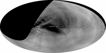
Figure 17. The difference map, CHIPASS (blurred to $35\hbox{$.\hspace{-2.22214pt}^\prime $}4$
) minus Reich et al. highlights residual artefacts in both maps. Inevitably, strong point sources fail to cancel exactly, but there is almost no sign of medium-scale cosmic emission. Note that blanked areas around saturated sources result from the smoothing operation. Linear greyscale from −0.5 to 0.5 K.
$35\hbox{$.\hspace{-2.22214pt}^\prime $}4$
) minus Reich et al. highlights residual artefacts in both maps. Inevitably, strong point sources fail to cancel exactly, but there is almost no sign of medium-scale cosmic emission. Note that blanked areas around saturated sources result from the smoothing operation. Linear greyscale from −0.5 to 0.5 K.
As an indirect measure of image fidelity, up to four orders of diffraction rings can be seen around Tau A, Ori A, and Virgo A. At least the first order diffraction ring can also be detected around Pictor A, Hydra A, 3C273, Hercules A, and 3C353. Three orders were also visible around W38 in the S-PASS difference map.
The following CHIPASS data products are available from www.atnf.csiro.au/research/CHIPASS/:
-
• The extended source map in Galactic coordinates on a Hammer-Aitoff projection as seen in Figure 15. This map, calibrated in mK full-beam brightness temperature, is the main product of this work.
-
• A subset of the above, the Galactic plane map, in Galactic coordinates but on a plate carrée projection spanning + 68° ⩾ ℓ ⩾ −180° with |b| < 10°. This map is provided specifically for studies of the many complex sources in the Galactic plane.
-
• The extended source map in J2000 equatorial coordinates on a plate carrée projection. This is the most suitable map to use for blurring the HPBW, or regridding onto other coordinate systems and map projections.
-
• The compact source map in Galactic coordinates on a Hammer-Aitoff projection as seen in Figure 1. This map, calibrated in Jy beam−1, is best suited for measuring point source positions and flux densities. It is independent of the calibrations needed for the extended source maps.
Each map was produced using all relevant HIPASS, ZOA, and Sculptor deep-field data. The compact source map also includes the Centaurus deep-field survey data. Each map has an associated relative sensitivity map akin to Figure 16. Table 4 summarises important map parameters.
Table 4. Summary of parameters relating to the full-sky, extended-source Hammer-Aitoff equiareal map.

†a Area of a top-hat function with the same peak height and volume as a Gaussian of specified FWHM (=π/(4ln 2) FWHM2).
†b Excluding the brightest 16 sources, which are saturated.
†c The robust measure of dispersion discussed in Section 3.4.
†d The imposed cut-off.
†e Number of input spectra (of either polarisation) used to compute the pixel value.
ACKNOWLEDGEMENTS
The HIPASS and ZOA surveys were the result of the tireless work, which extended over many years, of many collaborators and observers, including the ATNF electronics group who built the beautiful multibeam receiver and correlator, the Parkes Observatory support staff, and the original authors of the livedata and gridzilla software suites. For this work Stacy Mader’s assistance with the data archive is gratefully acknowledged.
This work is based on software packages provided by GNU/Linux, specifically the Debian distribution, and by the Comprehensive TeX Archive Network.
The Parkes radio telescope is part of the Australia Telescope National Facility which is funded by the Commonwealth of Australia for operation as a National Facility managed by CSIRO.


