


In clinical and epidemiological settings, where practicality and low cost are dominant issues and using a reference measurement method is not possible, reliable practical methods are needed to estimate body composition. Anthropometry has been used widely for many years as a simple method to assess body composition, and specifically total body fat content, which relates importantly to metabolic disease risks. BMI, skin-fold thicknesses, limb and trunk circumference, dual-energy X-ray absorptiometry (DXA) and bio-impedance methods have all been used in clinical settings and epidemiological surveys. Each of these methods has strengths and limitations, but all of them need to be calibrated against a reference method. In the past, the most commonly used methods were densitometry – using underwater weighing (UWW) – or computed tomographic (CT) imaging, but MRI is now the preferred reference method for body composition measurements at the organ level( Reference Heymsfield 1 ).
Using densitometry measurements to estimate total body fat as % body weight, Deurenberg et al. ( Reference Deurenberg, Weststrate and Seidell 2 ) used BMI, age and sex as variables to predict fat mass among 1229 men and women with a wide age range (7–83 years) and BMI (13·9–49 kg/m2). Anthropometric estimates of percentage body fat in adults had high correlations with UWW-measured total body fat (R 2 0·80) that were supported by cross-validations( Reference Deurenberg, Weststrate and Seidell 2 ). However, this study combined men and women, therefore possibly giving misleadingly high correlations, and it assessed bias by showing the relation among the difference between observed and predicted against observed total body fat measurement. This assessment method could show an association when there was none( Reference Bland and Altman 3 ). A better analysis method, as described by Bland–Altman, is to plot the difference against the average of the observed and predicted values( Reference Bland and Altman 3 ).
In 1996, Lean et al. ( Reference Lean, Han and Deurenberg 4 ) developed regression equations from simple anthropometric measurements to predict total body fat calculated from body density measured by UWW in eighty-four women and sixty-three men. The best simple prediction equations, with least bias and validated in a separate population sample, were from waist circumference adjusted for age (R 2 0·69 for men, 0·75 for women). This study also validated (for the first time) the widely used skinfold measurement predictions of total body fat published by Durnin and Womersley( Reference Durnin and Womersley 21 ), and found that waist circumference provided almost identical predictive power( Reference Lean, Han and Deurenberg 4 ).
In addition to predicting total body fat, waist circumference performed well in predicting total adipose volume in men. Ross et al. ( Reference Ross, Leger and Morris 5 ) investigated the relationship between anthropometric variables and MRI-measured total adipose tissue volume in twenty-seven healthy men. The combination of waist circumference and waist:hip ratio explained 91 % of the variation in total adipose tissue volume. Nevertheless, this equation was not cross-validated nor was the agreement between methods investigated.
Kvist et al. ( Reference Kvist, Chowdhury and Grangard 6 ) developed whole-body adipose tissue predictive equations from whole-body CT in seventeen men and ten women. After cross-validation in seven men and nine women, total adipose tissue volume was best predicted by weight and height with a standard error of difference≤11 %. The very small sample size is a serious limitation in this study; moreover, women with ulcerative colitis were pooled with healthy women, and then allocated to derivation and cross-validation groups. There was no assessment of agreement or biases( Reference Bland and Altman 7 ).
There are many uses for prediction equations, principally in epidemiology, to examine time trends in populations and to explore clinical and biomarker associations of adipose tissue or fat mass. At present, there are no clear guidelines about body composition prediction equations, which leave a potential for them to be developed or used inappropriately. When developing prediction equations, it is important first to consider the reliability of the reference method – for example, deciding between using whole-body v. regional MRI scans. Next, the size, appropriateness and representativeness of the derivation sample must be considered, to permit predictions across the range of values in the population of interest and the use of proper statistical analysis. Validation using separate data is an essential step, which has often been omitted: equations can only be considered ‘predictive’ in a sample or population separate from the derivation sample. How prediction equations should be used depends on what exactly is being predicted and how powerful and reliable the equations are in any specific setting. A common example of misused prediction equations is using BMI (a weak prediction equation for total body fat (R 2 67·0–74·5))( Reference Lean, Han and Deurenberg 4 ) to categorise the adiposity of individuals or as an adjustment for ‘obesity’ in regression analysis. Another example is confusing total body fat with total adipose tissue in applying prediction equations. The derivation and validation sample characteristics always introduce limitations such as the frequent lack of validation in the young or in older people and in different racial groups.
The present study was, therefore, designed to derive new prediction equations using simple anthropometric variables to estimate total adipose tissue mass (TATM) from MRI measurements and to validate them in an independent sample. We also compared the most widely used existing prediction equations for total body fat, estimated from UWW with estimates based on our MRI measurements of adipose tissue.
Methods
Data included in the derivation and validation studies were collected from adult subjects in whom the same measurements had been made by different investigators in studies conducted at New York Obesity Nutrition Research Center’s Body Composition Unit, St Luke-Roosevelt Hospital, New York. For both anthropometric and MRI measurements, readers were blinded (subjects names and anthropometric data were anonymised). Race/ethnicity was determined by self-report and included declaration of race/ethnicity for parents and grandparents. Variables were created for four race/ethnicity categories: Caucasian, African-American, Hispanic and Asian.
All the studies obtained written informed consent from the participants and were approved by the Institutional Review Board of St Luke’s-Roosevelt Hospital( Reference Heymsfield, Gallagher and Mayer 8 – Reference Bosy-Westphal, Schautz and Later 10 ).
Subjects
Derivation study sample
A total of 416 (222 women) subjects aged between 18 and 88 years, with BMI ranging from 15·9 to 40·8 (kg/m2) participated in several related studies between 2000 and 2004( Reference Heymsfield, Gallagher and Mayer 8 ). Subjects were classified as having no known or diagnosed diabetes, cancer, heart disease or any other health conditions that would affect body composition or fat distribution. All were ambulatory, weight-stable (<2 kg weight change in previous 6 months) adults, who underwent investigations that included anthropometry and whole-body MRI scanning. Four subjects were excluded from this sample because of technically poor or incomplete MRI scans.
Validation study sample
Data sets from two previous studies( Reference He, Heshka and Albu 9 , Reference Bosy-Westphal, Schautz and Later 10 ) were combined, giving a total of 204 subjects (110 women, ninety-four men). Subjects were recruited (study 1: 2001 to 2004( Reference He, Heshka and Albu 9 ), study 2: 2011( Reference Bosy-Westphal, Schautz and Later 10 )) through advertisements in local newspapers, internet and on flyers posted in the local community. A BMI (kg/m2) upper limit of 37 was set to accommodate the MRI scanner limitations. Participants were required to be ambulatory non-smokers, free of medical conditions or metabolic characteristics (abnormal thyroid or cortisol concentrations) that could affect the variables under investigation, weight stable (<2 kg change within past 6 months) and not regularly engaging in vigorous exercise. The subjects varied in age (18–86 years) and BMI (15·7–36·4 kg/m2) (Table 1). This final sample was carefully checked to ensure that there was no duplication of subjects between the derivation and validation samples. The validation sample was used to validate the newly derived equations and the existing equations of Lean et al. ( Reference Lean, Han and Deurenberg 4 ), Deurenberg et al. ( Reference Deurenberg, Weststrate and Seidell 2 ), Kvist et al. ( Reference Kvist, Chowdhury and Grangard 6 ) and Ross et al. ( Reference Ross, Leger and Morris 5 ).
Table 1 Subject characteristics and variables used for derivation and validation studies (Mean values and standard deviations, or percentages)

SM, skeletal muscle mass; TATM, total adipose tissue mass.
Measurements
MRI
All the data were collected in the same laboratory by an analysis team (n 3) for derivation and validation samples. For the 2011 study, a single MRI analyst performed the measurements. A 1·5 T MRI scanner (6x HORIZON; General Electric) was used for both the studies( Reference Song, Ruts and Kim 11 ). Whole-body MRI was carried out to identify and quantify total body and regional adipose tissue( Reference Shen, Wang and Tang 12 ). The procedure involved acquisition of approximately forty axial images of 10 mm thickness at 40 mm intervals throughout the whole body( Reference Song, Ruts and Kim 11 ). Cross-sectional images were analysed for subcutaneous adipose tissue, visceral adipose tissue, inter-muscular adipose tissue and total adipose tissue by three trained observers using VECT image analysis software (Slice-O-Matic), and total volumes were calculated as reported by Shen( Reference Shen, Wang and Tang 12 ). Intra-class correlation coefficients for agreement among multiple readers were subcutaneous adipose tissue 0·99 (95 % CI 0·81, 1·0) and visceral adipose tissue 0·95 (95 % CI 0·58, 0·99)( Reference Song, Ruts and Kim 11 ).
Anthropometric measurements
Three technicians, who were trained in the body composition laboratory, reported all the anthropometric data. Body weight was measured to the nearest 0·1 kg using a balance beam scale (Weight Tronix) with the subject wearing a hospital gown. A wall-mounted stadiometer (Holtain) was used to measure standing height to the nearest 0·1 cm. Anthropometric circumferences were obtained using a heavy-duty inelastic plastic fibre tape measure (Gulick II Tape Measure): waist circumference was measured from the midpoint between the lowest rib and the upper border of the iliac crest( Reference Wang, Zhu and Wang 13 ); hips circumference was measured between the level of the pubic symphysis and the greatest gluteal protuberance; mid-arm circumference was measured at the mid-point between the lateral tip of the acromion and the most distal point on the olecranon; mid-thigh circumference was measured at the mid-point between the inguinal crease and the proximal border of the patella; and the maximum girth of the calf was measured. The procedures outlined for anthropometric measurement sites and training were as outline in the ‘Anthropometric Standardization Reference Manual’( Reference Lohman, Roche and Martorell 14 ).
Statistical analysis
All the data sets had been previously checked and cleaned for errors of data entry, but were initially explored to confirm that all data ranges were plausible.
Assumptions for computations
Total adipose tissue mass
Measured whole-body adipose tissue volume, reported in litres, was converted to kilograms by multiplying volume of tissue by the reference density of adipose tissue: (0·92 g/l)( Reference Garrow 15 ) (Fig. 1).
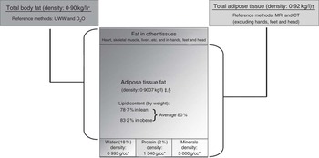
Fig. 1 Published assumptions and the relationship between total adipose tissue and total body fat. * Siri( Reference Siri 30 ), † Garrow( Reference Garrow 15 ), ‡ Fidanza et al. ( Reference Fidanza, Keys and Anderson 31 ), § Brozek et al. ( Reference Brozek, Grande and Anderson 32 ).
Total adipose tissue fat mass
Total adipose tissue fat mass was determined assuming the proportion by weight of the lipid fraction in adipose tissue to be 0·80( Reference Wang, Zhu and Wang 13 , Reference Snyder, Cook and Nsset 16 , Reference Sohlstrom, Wahlund and Forsum 17 ) (Fig. 1).
Prediction equation development
Multiple linear regressions generated equations, separately for males and females, to predict TATM measured by MRI. Eight anthropometric variables were considered to be of interest, on grounds of practicality for routine clinical and epidemiological work: age, weight, height and circumferences (hip, waist, thigh, arm and calf). Forward and backward stepwise regression analyses were performed (α to enter 0·15, α to remove 0·15) using the eight variables. The highest R 2 value of each set of stepwise regression was investigated further. Bland–Altman plots were used to explore distributions of errors( Reference Bland and Altman 7 ). Log-transformation was used to resolve skewness of the sample and investigate any relation in the Bland–Altman plot, by plotting the difference between the natural logarithm of MRI-measured TATM and the natural logarithm of predicted TATM against natural logarithm of the mean of the MRI-measured and predicted TATM( Reference Bland and Altman 7 ). To investigate the effect of adding the variable ‘Race’ (as applied in mixed US populations) to the equation, we used the derivation study sample, with the addition of the variable (Race) to our best derived equations for both men and women. Given that we had a categorical value (Race), ANCOVA general linear model was used.
The best derived prediction equations were validated using linear regression against whole-body MRI measurements in a separate validation sample. Bland–Altman plots were also created in the validation sample to determine levels of agreement between predicted and true MRI adipose tissue mass.
Standard error of the estimate (SEE) was used to define the accuracy of prediction equations. Judgement was based on comparison with similar published equations( Reference Deurenberg, Weststrate and Seidell 2 , Reference Lean, Han and Deurenberg 4 , Reference Ross, Leger and Morris 5 , Reference Kvist, Chowdhury and Grangard 6 ). To compare models, CV was calculated as the ratio of the SEE to the mean of the dependant variable. To investigate limits of agreements between MRI-estimated TATM and prediction equations, 95 % CI was used.
Association with other adipose tissue and body fat equations
Of the two total adipose tissue prediction equations, one was developed using CT scan( Reference Kvist, Chowdhury and Grangard 6 ) and the other using MRI( Reference Ross, Leger and Morris 5 ). These equations were compared with our TATM-derived prediction equation.
Two total body fat UWW-derived prediction equations( Reference Deurenberg, Weststrate and Seidell 2 , Reference Lean, Han and Deurenberg 4 ) were compared with our derived TATM after converting it to total adipose tissue fat mass (TATFM) using the following equation: (TATFM=TATM×0·80).
All the statistical analyses were carried out using Minitab® 16.2.0.0.
Results
Subject characteristics are shown in Table 1. Linear regression of single variables against MRI-measured TATM (Table 2) showed generally stronger correlations for women than for men, except for mid-calf circumference and waist:hip ratio.
Table 2 Explained variance (R 2) in MRI total adipose tissue mass (TATM) and whole-body skeletal muscle mass, from simple linear regressions in the derivation study
* Race included four categories, Caucasians, African-American, Asian and Hispanic. Race was analysed using general linear ANCOVA.
Equations for total adipose tissue mass
Derivation of prediction equations for total adipose tissue mass
Best equation for men (P1TATM)
The best variables after stepwise regression in men were body weight, waist circumference and hip circumference. Multiple regression gave high correlations, R 2 0·82, SEE 3·4 kg and CV 18 %, with narrow 95 % CI 17·5, 18·5 for an 18 kg adipose tissue measurement, yet 95 % prediction interval (PI) was high (95 % CI 11·2, 24·8) (Fig. 2(a)). Bland–Altman plots showed a negative relationship, P=0·004 (Fig. 2(b)); however, after log-transformation, this relationship was no longer present (P=0·728) and the negative slope ceased to exist (online Supplementary Appendix 1A). Limits of agreement based on one-sample t test were 95 % CI −0·03, 0·04. Adding race as a variable to the new equation did not affect the results for men (data not included).

Fig. 2 Derivation analysis in men: column 1 (a, c) shows scatter plots of MRI-measured total adipose tissue mass (TATM) (x-axis) against estimated TATM from prediction equations, whereas column 2 (b, d) shows Bland–Altman plots of difference between predicted and MRI-measured TATM (y-axis) against their mean (x-axis). Column 1 (e, g) shows scatter plots of MRI-measured total adipose tissue fat mass (TATFM) (x-axis) against estimated TATFM from prediction equations, whereas column 2 (f, h) shows Bland–Altman plots of difference between predicted and MRI-measured TATFM (y-axis) against their mean (x-axis). Lines represent mean difference of 0, regression (![]() ) and 95 % CI (
) and 95 % CI (![]() ) and prediction intervals (
) and prediction intervals (![]() ).
).
Simplest prediction equation in men (P2TATM)
The simplest prediction equation for TATM, providing a high predictive power in men included body weight, waist circumference and height. In Bland–Altman plots, skewness was resolved after log-transformation (online Supplementary Appendix 1B). There was no statistical difference between the best and simplest equation for men (Fig. 2(c) and (d)) (Table 3).
Table 3 Prediction equations (PE) for total adipose tissue mass (TATM) and total adipose tissue fat mass (TATFM) derived and validated in the present study (P), and validations of existing equations published by Lean et al. ( Reference Lean, Han and Deurenberg 4 ), Deurenberg et al. ( Reference Deurenberg, Weststrate and Seidell 2 ), Kvist et al. ( Reference Kvist, Chowdhury and Grangard 6 ) and Ross et al. ( Reference Ross, Leger and Morris 5 ) in menFootnote *

BW, body weight; CT, whole-body computed tomographic scan; d, derivation analysis; D, Deurenberg et al.; L, Lean et al.; K, Kvist et al.; NR, not reported; R, Ross et al.; UWW, underwater weighing; v, validation analysis.
* TATFM, TATM and BW in kg; waist, hip, height in cm, BMI (kg/m2); age in years and height measurement in m.
Best equation for women (P1TATM)
From the stepwise regression analysis, age, body weight, height and hip circumference gave the best correlations with TATM. As in men, multiple regression analysis gave a high correlation, R 2 0·89, with moderate SEE, 4·2 kg, and CV, 16 %, and 95 % CI did not vary much with fatness (95 % CI 9·3, 20·6) at the lower end, 20 kg TATM; however, 95 % PI was high (95 % CI 11·6, 28·4) at the upper end of adipose tissue mass, 35 kg TATM (95 % CI 34·2, 35·7 and 95 % PI 26·6, 43·4) (Fig. 3(a)). Bland–Altman plots showed a mean difference between predicted and measured values close to 0 (−0·002), (Fig. 3(b)). There was a slight negative correlation P=0·013, which was no longer present after log-transformation, P=0·804 (online Supplementary Appendix 1C). Limits of agreement based on one-sample t test were 95 % CI −0·021, 0·029. Adding the race variable did not change the results (data not included).

Fig. 3 Derivation analysis in women: column 1 (a, c) shows scatter plots of MRI-measured total adipose tissue mass (TATM) (x-axis) against estimated TATM from prediction equations, whereas column 2 (b, d) shows Bland–Altman plots of difference between predicted and MRI-measured TATM (y-axis) against their mean (x-axis). Column 1 (e, g) shows scatter plots of MRI-measured total adipose tissue fat mass (TATFM) (x-axis) against estimated TATFM from prediction equations, whereas column 2 (f, h) shows Bland–Altman plots of difference between predicted and MRI-measured TATFM (y-axis) against their mean (x-axis). Lines represent mean difference of 0, regression (![]() ) and 95 % CI (
) and 95 % CI (![]() ) and prediction intervals (
) and prediction intervals (![]() ).
).
Simplest prediction equation in women (P2TATM)
The simplest equation in women included body weight, age and height. Predictive power was almost identical to the best equation: R 2 0·88, SEE 4·2 kg and CV 16 % (Fig. 3(c)) (Table 4), skewness was resolved after log-transformation and 95 % CI was the same as P1TATM in women (Fig. 3(d)) (online Supplementary Appendix 1D).
Table 4 Prediction equations (PE) for total adipose tissue mass (TATM) and total adipose tissue fat mass (TATFM) derived and validated in the present study (P), and validations of existing equations published by Lean et al. ( Reference Lean, Han and Deurenberg 4 ), Deurenberg et al. ( Reference Deurenberg, Weststrate and Seidell 2 ) and Kvist et al. ( Reference Kvist, Chowdhury and Grangard 6 ) in womenFootnote *

BW, body weight; CT, whole-body computed tomographic scan; d, derivation analysis; D, Deurenberg et al.; L, Lean et al.; K, Kvist et al.; NR, not reported; UWW, underwater weighing; v, validation analysis.
* TATFM, TATM and BW in kg; waist, hip, height in cm; BMI (kg/m2); age in years, and height measurement in m.
† Nine women with ulcerative colitis were pooled with ten healthy women, nineteen women were ranked according to weight then allocated to derivation and cross-validation group.
Validation of derived equations to predict total adipose tissue mass
Validation of our best equations gave high correlations for both men and women (0·80 and 0·84, respectively). SEE for women was slightly lower than that for men (3·0 v. 3·7 kg) (Fig. 4(a) and 5(a)). CV decreased by 4 % in women and increased by 2 % in men. Limits of agreement in men was 95 % CI 24·7, 26·7 and 95 % PI 18·3, 33·1 and for women it was 95 % CI 24·1, 25·3 and 95 % PI 18·6, 30·7. Bland–Altman plots for women showed a slight positive relation, P=0·04, which was resolved after log-transformation, P=0·08 (Fig. 5(b)) (online Supplementary Appendix 1E). No skewness was seen in the Bland–Altman plots for men, and thus there was no need for transformation (P=0·67). There was a slight mean underestimation (−1·3 kg) compared with MRI-measured TATM in men, 95 % CI of the log-transformed equations in women based on one-sample t test were 95 % CI −0·023, 0·032, and in men limits of agreement based on one-sample t test without log-transformation were 95 % CI −2·4, −0·5 (Fig. 4(b) and 5(b)).

Fig. 4 Validation in men: column 1 (a, c) total adipose tissue mass (TATM) and (e, g) total adipose tissue fat mass (TATFM) are scatter plots of MRI-measured (y-axis) against estimated TATM and TATFM from prediction equations, whereas column 2 (b, d) TATM and (f, h) TATFM are Bland–Altman plots of difference between predicted and MRI-measured values (y-axis) against their mean (x-axis). Plots (a, b) represent results from the validation of our best equation in men (P1TATM). (c, d) Validation of our simplest equation (P2TATM). Plots (e, f) are our validation of our best TATFM equation (P1TATFM), and (g, h) our validation of our simplest TATFM equation (P2TATFM). Plots (m, n) represent our validation of Kvist TATM equation (P-Kvist), Plots (o, p) represent our validation of Ross TATM equation (P-Ross). Plots (i, j, k, l) represent our comparison with Lean et al.
(
Reference Lean, Han and Deurenberg
4
) and Deurenberg et al.
(
Reference Deurenberg, Weststrate and Seidell
2
) total body fat equations. For the plots with no significant slope, Bland–Altman plots show the mean difference with limits of agreement around the mean difference a test for bias (mean difference significantly different from 0) using the one-sample t test. For the plots with significant slope, Bland–Altman plots show the 95 % CI (![]() ) and prediction intervals (
) and prediction intervals (![]() ) around the regression (
) around the regression (![]() ) line. P values represent a test of significance of the slope. (b, d, f, h):
) line. P values represent a test of significance of the slope. (b, d, f, h): ![]() , mean difference;
, mean difference; ![]() , mean (2 sd).
, mean (2 sd).

Fig. 5 Validation in women: column 1 (a, c) total adipose tissue mass (TATM) and (e, g) total adipose tissue fat mass (TATFM) are scatter plots of MRI-measured (y-axis) against estimated TATM and TATFM from prediction equations, whereas column 2 (b, d) TATM and (f, h) TATFM are Bland–Altman plots of difference between predicted and MRI-measured (y-axis) against their mean (x-axis). Plots (a, b) represent results from the validation of our best equation in women (P1TATM). (c, d) represent our validation of our simplest equation (P2TATM). Plots (e, f) is our validation of our best TATFM equation (P1TATFM), and (g, h) our validation of our simplest TATFM equation (P2TATFM). Plots (I, J) represent our comparison with (Lean et al.
(
Reference Lean, Han and Deurenberg
4
)) total body fat equation (P-Lean), Plots (k, l) represent our comparison with (Deurenberg et al.
(
Reference Deurenberg, Weststrate and Seidell
2
)) total body fat equation (P-Deurenberg). Plots (m, n) represent our validation of (Kvist et al.
(
Reference Kvist, Chowdhury and Grangard
6
)) equation (P-Kvist). For the plots with no significant slope, Bland–Altman plots show the mean difference with limits of agreement around the mean difference a test for bias (mean difference significantly different from 0) using the one-sample t test. For the plots with significant slope, Bland–Altman plots show the 95 % CI (![]() ) and prediction intervals (
) and prediction intervals (![]() ) around the regression (
) around the regression (![]() ) line. P values represent a test of significance of the slope. (f, h):
) line. P values represent a test of significance of the slope. (f, h): ![]() , mean difference;
, mean difference; ![]() , mean (2 sd).
, mean (2 sd).
Validation of the simplest equations, without the variable hip circumference, also showed very similar results to the best equation for both men and women (Fig. 4(c), 4(d), 5(c) and 5(d)). In men, the mean was underestimated by −0·57 kg. In women, the sample was skewed, and after log-transformation the bias was no longer present (online Supplementary Appendix 1F).
Validation of published equations to predict total adipose tissue mass of Kvist et al. ( Reference Kvist, Chowdhury and Grangard 6 ) (P-Kvist)
The prediction equations originally derived and validated by Kvist et al. ( Reference Kvist, Chowdhury and Grangard 6 ) using CT scan and based on a mixed group of healthy adults and patients with ulcerative colitis were as follows:
Men: total adipose tissue (litres)=1·36 weight:height 42·0 (R 2=0·93)
Women: total adipose tissue (litres)=1·61 weight:height – 38·3 (R 2=0·96)
Correlations with our estimates based on the MRI measurements were greater in women than in men (R 2 0·82, 0·70, respectively); however, SEE was high (4·6 and 3·2 in men and women, respectively) and the limits of agreement were 95 % CI 24·5, 27·1 and 95 % PI 16·6, 34·9. The CV was higher in men than in women (27 v. 12 %) (Fig. 4(m) and 5(m)). Bland–Altman plots revealed significant biases, with significant positive relationships between differences and the average of observed and predicted values in women, which could not be corrected by log-transformations. From the Bland–Altman plot, limits of agreement in 18 kg fat men were 95 % CI −3·9, −1·8 and 95 % PI −12·9, 7·1 and in 30 kg fat men were 95 % CI −3·3, 0·3 and 95 % PI −11·6, 8·7.
These results indicate substantial bias and error (Fig. 4(n) and 5(n)).
Validation of published equation (total adipose tissue mass) of Ross et al. ( Reference Ross, Leger and Morris 5 ) (P-Ross, Men)
Ross et al. ( Reference Ross, Leger and Morris 5 ) derived a prediction equation from twenty-seven healthy men using MRI-measured adipose tissue: total adipose tissue (litres)=1·003×waist circumference−56·475×waist:hip ratio – 21·364 (d: R 2 0·91). Our validation of this equation showed good correlations and reasonable agreement – R 2 0·81, SEE=3·6 and CV=24 %. There was no relationship in the Bland–Altman plots to indicate bias, but there was a consistent underestimation: mean difference −5. Limits of agreement using one-sample t test were 95 % CI −5·5, −4·0 and from Bland–Altman plots were 95 % PI −12·02, 2·57 (Fig. 4(o) and (p)).
Equations to estimate total adipose tissue fat mass
To estimate TATFM, TATM was converted to TATFM using the factor 0·8( Reference Wang, Zhu and Wang 13 , Reference Snyder, Cook and Nsset 16 , Reference Sohlstrom, Wahlund and Forsum 17 ), TATFM=TATM×0·8.
Men (P1TATFM, P2TATFM)
Correlations were high in both equations with and without hip circumference (R 2 0·82 and 0·79) for P1TATFM and P2TATFM, respectively, SEE and CV ((2·8, 3·0) and (18, 20 %)) (Fig. 2(e) and (g)). The width of 95 % CI was 1·4 in both P1TATFM and P2TATFM, and the width of 95 % PI was 11·9 and 12·2, respectively, for an 18 kg measurement of TATFM. In the Bland–Altman plots, the mean difference was close to 0 (−0·12 and 0·00) with slight bias (P=0·003, 0·001) that was corrected by log-transformation (P=0·603 and 0·137, respectively) (Fig. 2(f) and (h)) (online Supplementary Appendix 1G, 1H). Validation of men TATFM equations showed high correlations for both equations with and without hip circumference (R 2 0·80 and 0·79, respectively), SEE (3·0) and CV (20 %). Limits of agreement of 18 kg measured TATFM were 95 % CI 18·1, 19·5 and 95 % PI 12·9, 24·8 in P1TATFM and were 95 % CI 17·5, 18·9 and 95 % PI 12·1, 24·3 in P2TATFM. No bias was seen in Bland–Altman plots, and limits of agreement based on one-sample t test were 95 % CI −1·75, −0·51 and 95 % CI −1·10, 0·17, respectively (Fig. 4(e)–(h)).
Women (P1TATFM, P2TATFM)
No difference in correlation, SEE and CV between best and simplest TATFM prediction equations was observed (Fig. 3(e) and (g)). Bland–Altman plots showed slight bias (P=0·013, 0·008), which was resolved by log-transformation (Fig. 3(f) and (h)) (online Supplementary Appendix 1I, 1J). Our validation of women’s adipose tissue fat mass equations showed high correlations (R 2 0·84) and good SEE (2·4, 2·5) and CV (12, 13 %) as well as no bias in Bland–Altman plots (95 % CI −0·5, 0·6 and 95 % PI −5·1, 5·2). Limits of agreement based on one-sample t test were 95 % CI −0·30, 0·70 and 95 % CI −0·13, 0·89 in P1TATFM and P2TATFM, respectively.
Association with published equations to predict total body fat of Lean et al. ( Reference Lean, Han and Deurenberg 4 ) (P-Lean)
Estimates of TATFM from MRI were compared with the simplest prediction equations for total body fat, derived and validated, using UWW by Lean et al. ( Reference Lean, Han and Deurenberg 4 ).
Men total body fat (%)=0·567 waist (cm)+0·101 age (years)−31·8 (d: R 2 0·78, v- R 2 0·69).
Women total body fat (%)=0·439 waist (cm)+0·221 age (years)−9·4 (d: R 2 0·70, v- R 2 0·75).
Correlations were higher in men (R 2 0·80) than in women (R 2 0·76), and SEE was 3·0 kg for both men and women (Fig. 4(i) and 5(i)).
Assuming that TATM is comprised of 80 % fat( Reference Garrow 15 ), we estimated TATFM by multiplying TATM by 0·80, and related them with the estimates of Lean et al. ( Reference Lean, Han and Deurenberg 4 ) of total body fat, which showed mean overestimation of TATFM by 2·53 kg in men and by 4·89 kg in women (Fig. 4(j) and 5(j)). There was some skewing (P=0·000), and Bland–Altman plots showed relationships between the mean and the difference, which persisted after log-transformation (P<0·001) in men but not in women (P=0·188 after log-transformation) (online Supplementary Appendix 1K) (95 % PI −0·09, 0·56). Limits of agreement based on one-sample t test in women were 95 % CI 0·197, 0·259. In men with lower values of TATFM (18 kg), 95 % CI 1·12, 3·56, and in men with higher values of TATM (35 kg) 95 % CI 5·68, 9·45.
Association with published equations to predict total body fat by Deurenberg et al. ( Reference Deurenberg, Weststrate and Seidell 2 ) (P-Deurenberg)
Published equations by Deurenberg et al. ( Reference Deurenberg, Weststrate and Seidell 2 ) were as follows:
Total body fat (%)=1·20×BMI+0·23×age (years)−10·8×sex−5·4 (1 for men, 0 for women).
The Deurenberg equation was more reliable in women than in men in terms of R 2 (0·78 v. 0·70), SEE (2·9 kg v. 3·6 kg) and CV (12 v. 19 %) (Fig. 4(k) and 5(k)), with limits of agreement based on 95 % PI 7·6, 22·0 and 9·7, 21·2 for men and women, respectively. Our derived estimates of TATFM showed mean overestimation of TATFM as predicted by Deurenberg et al. by 3·52 in men and 4·13 in women. There was some skewing in the Bland–Altman plots, revealing a minor negative relation in both men and women (P=0·04), (P<0·01) (Fig. 4(l) and 5(l)), which was overcome by log-transformation (online Supplementary Appendix 1L, 1M). Limits of agreement based on one-sample t test were 95 % CI 0·15, 0·27 and 0·16, 0·22 in men and women, respectively.
Discussion
BMI is still the most popular method for classifying fatness and thinness, despite its rather weak correlation with body fat content( Reference Lean, Han and Deurenberg 4 , Reference Gallagher, Visser and Sepulveda 18 , Reference Bedogni, Pietrobelli and Heymsfield 19 ) and its failure to distinguish fat mass from muscle mass, which have opposite implications for health and well-being. At present, most national survey analyses report BMI and equate BMI>30 with ‘obesity’. That has led to all sorts of misinterpretations of survey data( Reference Romero-Corral, Montori and Somers 20 ). Body fat is better estimated using the sum of four skinfold thickness measurements( Reference Durnin and Womersley 21 ), but this method requires training and has a poor record for inter-observer variability( Reference Wang, Thornton and Kolesnik 22 , Reference Al-Gindan, Hankey and Leslie 23 ). As a single measure, waist circumference alone is simpler and the most reliable circumference measurement, which gives similar prediction of total body fat to skinfold measurements( Reference Lean, Han and Morrison 24 , Reference Han, van Leer and Seidell 25 ). These methods were all based on estimation of total body fat from UWW using the two-compartment model. Adipose tissue, which is conventionally assumed to contain 80 % of total body fat( Reference Shen, Wang and Punyanita 26 ) (Fig. 1), can be directly and accurately measured using modern imaging methods. Equations have been published using anthropometry based on CT scanning in a very small study( Reference Kvist, Chowdhury and Grangard 6 ), but MRI has been considered as the reference for adipose tissue measurement for many years now, and anthropometric prediction equations have not previously been validated against whole-body MRI.
We have explored the use of simple anthropometric measurements that are made routinely in health surveys to predict TATM as estimated by MRI as the reference method. We assessed new equations against four previously published methods based on different reference methods, Lean et al. ( Reference Lean, Han and Deurenberg 4 ) and Deurenberg et al. ( Reference Deurenberg, Weststrate and Seidell 2 ) for total body fat based on UWW, Kvist et al. ( Reference Kvist, Chowdhury and Grangard 6 ) for TATM based on CT and Ross et al. ( Reference Ross, Leger and Morris 5 ) for TATM based on MRI, but never validated them (Tables 3 and 4). The different reference methods have never been directly compared in the same subjects, but the published anthropometric equations derived and validated using these different methods all gave broadly similar results when applied to MRI measurements in the present study. The new MRI-derived equations had similar R 2 but showed less errors and biases than the existing published methods. For published TATM equations in men, both Kvist and Ross equations underestimated TATM by −2·86 and −4·72, respectively. In women, Kvist et al’s. equation overestimated TATM by 3·08. As for total body fat, equations of both Lean et al. ( Reference Lean, Han and Deurenberg 4 ) and Deurenberg et al. ( Reference Deurenberg, Weststrate and Seidell 2 ) overestimated TATFM in men, showing better results after log-transformation in women.
The equations provide sufficient prediction of TATM in both sexes for many epidemiological purposes, with R 2 being better than BMI, but there are certain limitations. Women showed consistently stronger correlations between anthropometry and TATM than men (Table 2). This may be expected as women have greater fat masses than men and greater variation between individuals which allow higher R 2 values. The converse applies for prediction equations to estimate whole-body muscle mass, where men have consistently higher correlations with anthropometry( Reference Al-Gindan, Hankey and Govan 27 ). For women, the main predictor of TATM was body weight, whereas for men it was waist circumference (Table 2).
Comparisons of the new equations with those of Lean et al. ( Reference Lean, Han and Deurenberg 4 ) and Ross et al. ( Reference Ross, Leger and Morris 5 ), where both included waist circumference, showed higher correlations for men (Table 3). On the other hand, the Deurenberg et al. ( Reference Deurenberg, Weststrate and Seidell 2 ) and Kvist et al. equations, which used BMI and weight/height, respectively as variables, both showed higher correlations in women than in men (Table 4).
The relationship between BMI and body fat has been studied extensively( Reference Gallagher, Visser and Sepulveda 18 , Reference Forbes 28 ). In our samples, BMI showed reasonable correlation in the linear regression analysis with measured TATM in women (R 2 0·82) but showed only moderate correlation in men (R 2 0·66). When BMI was added to the stepwise regression analysis, it did not appear to be significant within the best equations (Table 3). Similarly, using equations based on BMI, Deurenberg et al. ( Reference Deurenberg, Weststrate and Seidell 2 ) found only moderate correlations with estimated TATFM (0·70–0·78).
Waist:hip ratio has shown conflicting results in its relationships with metabolic illness and with measured adipose tissue( Reference Burton, Gray and Webb 29 ). Ross et al. ( Reference Ross, Leger and Morris 5 ) reported that waist:hip ratio correlated strongly with MRI-measured total adipose tissue, but R 2 was only 72 %. Adding waist circumference increased the correlation substantially to explain 91 % of the variance. The same was observed in our data set. After stepwise regression, the best variables for men included waist circumference, waist:hip ratio and body weight (R 2 0·82, SEE=3·4) (figures not included), but compared with our equations no significant difference was seen, and in terms of practicality we decided to use the equations without the waist:hip ratio. In the present study, waist:hip ratio was not a significant predictor of TATM in women (linear regression R 2 0·025).
The best equations for both men and women included hip circumference. The additional predictive power from including hip circumference was relatively small, probably because hip circumference is more strongly related to gluteal muscle mass( Reference Al-Gindan, Hankey and Govan 27 ) outside extreme obesity.
As the measurement of hip circumferences requires removal of some clothing, and is less often performed in large health surveys, we evaluated prediction of MRI-TATM and TATFM from simpler, more practical, measures such as age, height, weight and waist. From these variables, the best prediction of TATM in men was from body weight, waist circumference and height, and in women it was from body weight, height and age. These equations performed well in the validation analyses, with very similar predictive power to our ‘best’ derived equations (Table 3).
Log-transformations of the data were needed in most of our Bland–Altman plots to account for significant relationships between mean difference and average, due to a combination of non-constant variation and skewness in the predicted and MRI measurements. This would be expected as there were fewer subjects in the samples who had large fat masses than with low or average fat mass measurements.
It is perhaps surprising that age did not appear as a significant variable in the best prediction equations for men. This could be due to the relatively small number of adults aged over 60 years (twelve subjects) in our derivation sample, but in general the use of physical measures with high prediction accounted for differences related to ageing. The same applied to the race variable, which is valuable for defining race but problematic in mixed populations.
Strength and limitations of the present study
Our study included a larger number of subjects than previous studies to develop anthropometric prediction equations, which allowed a more robust analysis of agreements and biases. Our data were from diverse samples in terms of age and of racial groups. It was reassuring that adding a term for racial group into our model did not add predictive value, indicating that simple anthropometric measures accounted for inter-racial differences in body composition. Other predictive equations that did not include body circumferences needed a term for race to be included, which presents practical difficulties for ascertainment, particularly in mixed-race populations. Ethnicity, usually self-attributed, is even trickier. Gallagher et al. ( Reference Gallagher, Visser and Sepulveda 18 ) studied a cohort of 706 adults using a four-compartment body composition model to estimate total body fat as a percentage of body weight. They concluded that BMI is sex and age dependent when used as an indicator of body fat, but that BMI is independent of ethnicity in Caucasian and African-American adults. It is important for our validation studies that the measurements were all made following an identical protocol to the derivation studies. Ideally these measures would have been made by completely independent investigators, and perhaps using different equipment, in order to confirm transferability of the method. However, the similarities in predictions of MRI-measured TATM and TATFM with the previously published equations using different methods allow confidence that our methods are likely to be reliable when applied in different settings.
The relatively low number of ageing adults in our derivation sample may have introduced bias, Ideally, the number of subjects over sixty should be higher.
It is important to recognise that adipose tissue fat mass measured by MRI correlates with ‘fat’ as estimated by two-component methods such as DXA or UWW, but they estimate different targets. In our analysis, we used two assumptions that have been used extensively in the literature( Reference Deurenberg, Weststrate and Seidell 2 – Reference Kvist, Chowdhury and Grangard 6 ). To convert total adipose tissue in volume to mass in kg we multiplied by 0·92, and to convert TATM to TATFM we multiplied TATM by 0·8 (Fig. 1). These assumptions incur limitations, particularly when using a single factor for all the subjects for estimating the fat content of adipose tissue, as this is likely to vary with degree of fatness. MRI does not capture small fat depots below the level of resolution within muscles, liver, etc, and hands, feet and head are commonly excluded from whole-body MRI. Thus, in our analyses, total body fat derived from UWW( Reference Bland and Altman 7 , Reference He, Heshka and Albu 9 ) correlated strongly with TATFM measured by MRI (R 2 0·70–0·80), but there were differences between them, rising with fatness. Bland–Altman plots (Fig. 4(j), 4(l), 5(j) and 5(l)) showed considerable variability, but the difference between these estimates was about 1 kg for men and 2 kg for women for an average thin individual with 15 kg TATFM and 5–7 kg for an average obese individual with 37 kg TATFM.
We could not interpret the effects of illness, physical disability or extremes of age within our data set. Further validation would be advisable for the equations to be used in these conditions.
Conclusion
New equations, using simple anthropometric measurements and without need for a race variable, estimated MRI-measured TATM with higher correlations and better agreements than existing equations. The new equations for TATM, with standard conversions to estimate total body fat, generated broadly similar figures to published anthropometric equations for total body fat. The degree of individual variation, as with previous prediction equations, implies that they should not be used for clinical or diagnostic purposes, but they have value for use among groups and populations, as well as to estimate body fat substantially better (modestly greater R 2) than BMI alone.
Acknowledgements
The authors thank Martin Hoefler for data collection and Maureen McNee for secretarial assistance.
This work forms part of a PhD programme of Yasmin Algindan at the University of Glasgow, supported by a grant from the University of Dammam, Saudi Arabia.
All authors contributed to study design, critically reviewed drafts and approved the final version of the manuscript. S. H. and D. G. contributed to data collection studies. Y. Y. A. carried out data analysis with statistical guidance from L. G.
There are no conflicts of interest to declare.
Supplementary material
For supplementary material/s referred to in this article, please visit http://dx.doi.org/doi:10.1017/S0007114515003670


