


Introduction
Vertebrate bone tissue microstructures reveal ontogenetic status, physiology, annual growth rate, and sexual maturity (Cormack Reference Cormack1987; Francillon-Vieillot et al. Reference Francillon-Vieillot, de Buffrenil, Castanet, Geraudie, Meunier, Sire, Zylberberg and de Ricqlès1990; Games Reference Games1990; de Margerie et al. Reference de Margerie, Robin, Verrier, Cubo, Groscolas and Castanet2004; Schweitzer et al. Reference Schweitzer, Wittmeyer and Horner2005; Montes et al. Reference Montes, Castanet and Cubo2010), thereby permitting life history reconstructions of animals long extinct. Such analyses are applied to fossils of non avian dinosaurs, but small sample sizes can lead to inaccurate life history summaries. A laterally extensive monodominant bonebed, yielding thousands of fossils from the hadrosaurid dinosaur Maiasaura peeblesorum, offers a unique opportunity for large scale histologic analysis of an extinct taxon. Here we present a comprehensive growth series analysis of Maiasaura peeblesorum. Our study is different from other large scale paleohistology studies because it represents the largest single element, single taxon, and single population osteohistology synthesis to date for an extinct tetrapod. Additionally, every skeletal element sampled preserves the entire growth mark record, so that no retrocalculations for age determination were required for any specimen in our study. We hypothesize that our ontogenetic sample size of 50 histologically examined tibiae will permit more meaningful interpretations of ontogenetic growth, individual variation, and population biology, while allowing us to test established extinct tetrapod osteohistology hypotheses and assumptions that are based on less data.
Fossil remains of Maiasaura from a nesting horizon (Museum of the Rockies locality TM-160) in the Campanian Two Medicine Formation of Montana initially attracted scientific attention by providing the first evidence that at least some dinosaur taxa nested in colonies and that the altricial hatchlings were cared for by adults (Horner and Makela Reference Horner and Makela1979; Barreto Reference Barreto1997; Horner et al. Reference Horner, Padian and de Ricqlès2001). In the years that followed, Maiasaura specimens collected from a bonebed (Museum of the Rockies localities TM-003, TM-151, TM-158) overlying the nesting horizon revealed an ontogenetic shift from bipedality to quadrupedality (Dilkes Reference Dilkes2000, Reference Dilkes2001), intraskeletal variation in bone apposition rates, and maximum growth rates similar to those observed in extant large bodied mammals and birds (Horner et al. Reference Horner, de Ricqlès and Padian2000).
For the present study, samples of 50 Maiasaura tibiae were histologically examined to assess individual variation in growth and to produce the largest sample set to date for a dinosaur population biology synthesis. The tibia sample derives from decades of collecting from the Maiasaura bonebed, which spans at least two square kilometers and contains thousands of disarticulated Maiasaura skeletal elements (Varricchio and Horner Reference Varricchio and Horner1993) with very little time averaging (Trueman and Benton Reference Trueman and Benton1997). The tibia sample encompasses early juveniles (~3.0 m in body length) to skeletally mature adults (>7 m in body length) (Horner et al. Reference Horner, de Ricqlès and Padian2000). No perinatal material is present in the bonebed, so to construct a complete ontogenetic growth history we include a perinatal tibia from the nesting horizon for hatchling measurements.
The level of analysis provided by this large sample size allows more statistical strength in calculations of annual growth than previous large scale studies, and is based on the bone tissue of individual tibiae without requiring retrocalculations to account for any missing years of growth. Such a sample reveals ontogenetic patterns and individual variation easily overlooked with smaller sample sets. The statistical power provided by a sample of 50 tibiae (Steinsaltz and Orzack Reference Steinsaltz and Orzack2011) also permits more meaningful hypotheses of dinosaur survivorship curves. Our life history synthesis incorporates and builds upon previous Maiasaura studies (Horner and Makela Reference Horner and Makela1979; Horner Reference Horner1982, Reference Horner1983; Varricchio and Horner Reference Varricchio and Horner1993; Barreto Reference Barreto1997; Horner Reference Horner1999; Dilkes Reference Dilkes2000; Horner et al. Reference Horner, de Ricqlès and Padian2000; Dilkes Reference Dilkes2001; Horner et al. Reference Horner, Padian and de Ricqlès2001) and with the addition of the data acquired here, Maiasaura becomes the most ontogenetically well understood dinosaur species, allowing the most thorough evaluation of the life history of any extinct tetrapod thus far.
Institutional Abbreviations
MOR, Museum of the Rockies; ROM, Royal Ontario Museum; YPM-PU, Princeton University collections now curated at the Yale Peabody Museum.
Materials and Methods
Maiasaura peeblesorum skeletal elements, including the tibiae used in this study, were collected over a period of more than thirty years from three bonebed localities (MOR localities TM-003, TM-151, TM-158) within the Two Medicine Formation in an area of badland exposures approximately 19 km west of Choteau, Montana. The TM-003 locality is approximately 153 m northwest of TM-158, and approximately 629 m southeast of TM-151. Although erosion along the Willow Creek anticline geographically separates the sites, a bentonite layer is present approximately 4.3 m above all three localities (Lorenz and Gavin Reference Lorenz and Gavin1984; Varricchio et al. Reference Varricchio, Koeberl, Raven, Wolbach, Elsik and Miggins2010) and the sites are stratigraphically correlated (Schmitt et al. Reference Schmitt, Jackson and Hanna2014), representing a single 0.4–1.5 m thick bonebed, laterally traceable for approximately 2 km (Schmitt et al. Reference Schmitt, Jackson and Hanna2014). The bentonite layer is dated to 75.92±0.32 Ma (using the standard of MMhb-1=523.1 Ma) (Varricchio et al. Reference Varricchio, Koeberl, Raven, Wolbach, Elsik and Miggins2010). The presence of red beds, caliche horizons, and grey to red mudstones suggests that the Two Medicine Formation was deposited during semi arid conditions that included a long dry season and warm temperatures (Lorenz and Gavin Reference Lorenz and Gavin1984).
Hadrosaur bones dominate the bonebed, and Maiasaura peeblesorum is the only hadrosaurid taxon identified to the species level; there is no evidence of a second hadrosaurid taxon being present. A study by Schmitt et al. (Reference Schmitt, Jackson and Hanna2014) examined 189 previously excavated bones from various localities in the bonebed as well as 58 bones recovered from a 2 m2 test pit near TM-003. From the 247 skeletal elements examined, 171 (69.2%) are referred to Hadrosauridae, 15 (6.1%) to Maiasaurinae (sensu Horner Reference Horner1992, currently Brachylophosaurini sensu Gates et al. Reference Gates, Horner, Hanna and Nelson2011), and seven (2.8%) assigned to Maiasaura peeblesorum. The sample also included five theropod (2%) and 49 (19.8%) unidentified skeletal elements (Schmitt et al. Reference Schmitt, Jackson and Hanna2014). Fossils referred to as Maiasaura collected from these bonebed localities include unassociated cranial, axial, and appendicular skeletal elements.
The bonebed was most likely the result of a sediment gravity flow that varied temporally and spatially between a non cohesive debris flow and a hyperconcentrated flow (Schmitt et al. Reference Schmitt, Jackson and Hanna2014). A small component of the bonebed assemblage is likely made of bone incorporated from shallow scouring (10–30 cm in depth) of the underlying floodplain deposit substrate. Modern rates of floodplain sediment accumulation suggest a minimum of 10−2 years of time averaging for the exhumed skeletal elements (Schmitt et al. Reference Schmitt, Jackson and Hanna2014). Based on a lack of significant weathering features, the majority of hadrosaurid bones in the bonebed represent a minimal surface residence time of 0.1–10 years (Rogers Reference Rogers1993; Schmitt et al. Reference Schmitt, Jackson and Hanna2014). Geochemical analyses (Trueman Reference Trueman1999) also suggest this is a transported, weakly time averaged assemblage.
Ecological interpretation of tibia age frequency distribution, consisting largely of the very young and fewer adults or near adult animals (Fig. 1), is neither strongly attritional nor catastrophic. This is because the sample size of non juveniles is low enough that the abundances are not statistically significant, which could mask a catastrophic age profile. However, as was also suggested in Schmitt et al. (Reference Schmitt, Jackson and Hanna2014), we interpret the nearly monodominant nature of the bonebed, its fossil density, and weak time averaging as representing one or more transported catastrophic death episodes possibly related to drought or disease (Rogers Reference Rogers1990; Varricchio and Horner Reference Varricchio and Horner1993; Schmitt et al. Reference Schmitt, Jackson and Hanna2014) that selectively targeted weaker animals. Of any age grouping, those within their period of “peak performance” (i.e., when survival and reproductive rates are highest (Jones et al. Reference Jones, Gaillard, Tuljapurkar, Alho, Armitage, Becker, Bize, Brommer, Charmantier, Charpentier, Clutton-Brock, Dobson, Festa-Bianchet, Gustafsson, Jensen, Jones, Lillandt, McCleery, Merila, Neuhaus, Nicoll, Norris, Oli, Pemberton, Pietiainen, Ringsby, Roulin, Saether, Setchell, Sheldon, Thompson, Weimerskirch, Jean Wickings and Coulson2008; Nussey et al. Reference Nussey, Wilson, Morris, Pemberton, Clutton-Brock and Kruuk2008; Nussey et al. Reference Nussey, Kruuk, Morris, Clements, Pemberton and Clutton-Brock2009)) were most likely to survive the events, and are therefore not strongly represented within the assemblage. Thus, even if the cause of death was catastrophic, it could have been age selective, producing an age profile more similar to an attritional assemblage. Regardless of cause of death, due to low time averaging, we consider this bonebed to represent a population of Maiasaura that experienced similar seasonal environmental stresses over a geologically brief period of time, so that observed differences in bone microstructure should be influenced largely by individual genetic variability in growth and less so by environmental differences.

Figure 1 Histogram of measured Maiasaura tibia lengths and corresponding ages obtained from growth mark counts. Over half of the tibiae in the sample were from individuals less than one year of age. Of the remaining 19 tibiae, five were from individuals two years of age; three year olds were absent; and the rest were from individuals between four and 15 years of age (n=50).
From the fossils collected, 50 of the most complete tibiae (MOR 005 and MOR 758) were used in this study. Due to several factors, it is highly unlikely that any two contralateral tibiae included in our study were from the same individual. Such factors include: the density of Maiasaura fossils in the bonebed; the completely disarticulated nature of all the elements documented; the lateral extent of the bonebed; and the geographically (but not stratigraphically) separate sites within the bonebed from which specimens were collected. Therefore we report that the tibia sample set represents a minimum of 32 individuals (based on number of right tibiae) to set a lower limit on the number of individuals included in this study, but we will for the purposes of this paper consider each of the 50 tibiae to represent a single individual.
To make the results of bone microstructure analyses comparable across studies, researchers often select the femur for sectioning. But as with all hadrosaurids, the fourth trochanter in the femur of Maiasaura extends to nearly half the length of the diaphysis. This bony process is remodeled frequently during growth, thus affecting the visibility of primary tissue along most of the diaphyseal length. The tibia was chosen for analysis because it lacks such a process and is therefore less subject to extensive remodeling. Although there is variation in the apposition rates of different bones within a skeleton (Horner et al. Reference Horner, de Ricqlès and Padian1999; Cullen et al. Reference Cullen, Evans, Ryan, Currie and Kobayashi2014; Woodward et al. Reference Woodward, Horner and Farlow2014), this study samples only tibiae in order to directly compare variability present in a single element across multiple individuals. Along with the femur, the tibia tends to provide the most consistent skeletochronological results (Horner et al. Reference Horner, de Ricqlès and Padian1999), allowing reasonable estimates of maximum growth rates.
Tibiae collected from the bonebed and used in this project were numbered T1 through T50. Each was photographed and hand traced in lateral view prior to thin sectioning. The straight line distance from the anterior edge of the cnemial crest to the distal tip of the lateral malleolus was recorded (n=35) and conservative length estimates were made (Supplementary Table 1) in cases where either epiphysis was incomplete (n=13). Only three tibiae (T34, T49, T50) within the sample were too incomplete for reasonable length estimates.
A section of the diaphysis containing the least circumference (location determined by using a fabric tape measure) for each tibia was removed using a wet tile saw fitted with a continuous rim diamond blade, and then prepared following Lamm (Reference Lamm2013). The location of the least diaphyseal circumference was found to vary between 36.5% and 61.4% (x=48.8%) the length of the tibia as measured from the end of the lateral malleolus, regardless of ontogenetic status (Supplementary Fig. 1). Two transverse sections from the tibial shaft, each approximately 0.3 cm in thickness, were removed to either side of the line of minimum diaphyseal circumference. In most cases, only one of the two slices was completely processed for analysis while the second was held as a duplicate.
Completed slides were examined at either 10× or 40× total magnifications using a Nikon Optiphot-Pol polarizing microscope. Photomicrographs of the entire sections were taken incrementally using a Nikon DS-Fi1 digital sight camera, and compiled using NIS-Elements BR 3.0 software to create a single image from multiple photographs. Thus, these composite images often have a mosaic appearance. Transverse section periosteal surface circumferences as well as circumferences of medullary cavities and lines of arrested growth (LAGs) were traced in Adobe Photoshop CS3. Qualitative descriptions of bone tissue organization and vascular canal orientation apply the terminology from Francillon-Vieillot et al. (Reference Francillon-Vieillot, de Buffrenil, Castanet, Geraudie, Meunier, Sire, Zylberberg and de Ricqlès1990). Lines of arrested growth were identified as narrow (approximately between 10 and 30 μm thickness) black rings encircling the cortex, separating bone laminae on either side. In extant vertebrates, a LAG is a hypermineralized tissue representing the periosteal surface during temporarily arrested growth, and having an annual periodicity in extant vertebrates for which data exist (Peabody Reference Peabody1961; Castanet et al. Reference Castanet, Francillon-Vieillot, Meunier and de Ricqlès1993; Köhler et al. Reference Köhler, Marin-Moratalla, Jordana and Aanes2012). Therefore, we assume the same cause and periodicity holds true for LAGs found in Maiasaura. The LAGs in Maiasaura tibiae never cross cut bone laminae but followed them, and passed around vascular canals rather than through them. Unless obfuscated by diagenetic crushing, periosteal surface erosion, or secondary reconstruction, cortical LAGs could be fully traced. Only within the closely spaced LAGs representing the external fundamental system (EFS) of skeletally mature adults (Cormack Reference Cormack1987; Castanet et al. Reference Castanet, Newman and Girons1988) were growth marks difficult to fully trace due to their close spacing, splitting, or merging.
Another way in which the Maiasaura sample set is unique is that each specimen contains a complete LAG record. This is true in even the largest, skeletally mature specimens that are not diagenetically altered. In the large specimens, secondary remodeling and medullary expansion only partially obliterate the innermost LAG. The circumference of this partial innermost LAG corresponds with the shape and circumference of the largest tibiae for which no LAGs are present (i.e., juveniles dying just prior to the close of their first year of growth). This test therefore confirms that a full LAG record is preserved in large tibiae and makes the need for retrocalculations of missing LAGs unnecessary.
Periosteal and LAG circumferences, as well as the total area of the transverse section enclosed by the circumferences (here termed cortical area), were quantified using NIH ImageJ (Rasband 1997–Reference Rasband2014) and the BoneJ plugin (Doube et al. Reference Doube, Kłosowski, Arganda-Carreras, Cordelières, Dougherty, Jackson, Schmid, Hutchinson and Shefelbine2010) (Supplementary Table 1; Supplementary Table 2). High resolution versions of images discussed in this manuscript are accessible on MorphoBank (www.morphobank.org), project number P1139. Images of full transverse sections of three tibiae are also accessible in the same MorphoBank project. These include T16 (Morphobank image M326121), with no LAGs; T31 (M340003), with two LAGs; and T46 (M340007), with nine LAGs in the cortex and four in the EFS.
Individual average cortical apposition rates were calculated (Table 1) for each year of growth by using tibiae possessing LAGs as well as complete, uncrushed transverse diaphyseal sections (n=9). The distances along major and minor axes from the geometric centroid to the first LAG were measured and averaged to obtain a cortical thickness (Supplementary Table 3). This procedure was repeated for each consecutive LAG so that average annual apposition for each individual could be determined. Annual apposition was then converted to a daily rate (μm/day) based on a 365 day year, to allow direct comparisons with extant taxa (Myhrvold Reference Myhrvold2013). Maximum average daily apposition rates were also calculated (Table 1), assuming a three month (90 day) growth hiatus as determined for extant bovids (Köhler et al. Reference Köhler, Marin-Moratalla, Jordana and Aanes2012). As an alternative, yearly increase of growth hiatus duration was calculated (Table 1) assuming that apposition rate is constant throughout ontogeny and that it is the growth hiatus that increases as individuals age. For each scenario, apposition rates of cortical thickness between the outermost LAG and the periosteal surface were not calculated as this thickness does not represent a single year of growth (either less than a year in growing animals, or many years if the external fundamental system is present).
Table 1 Changes in Maiasaura bone tissue apposition rate based on zonal bone thickness. Rates are measured in micrometers per day. The "Conventional apposition rate" reports the daily apposition rate of bone if it were deposited continuously throughout a 365-day year, and is the method used in previous dinosaur cortical apposition rate studies. The "90-day hiatus" represents the daily apposition rate of bone deposited continuously throughout the growth season, with zero apposition during an estimated 90-day unfavorable season. "Increasing hiatus" instead assumes a constant apposition rate of 84.8 µm/day during 365 days of the first year, then maintaining the same rate during the growing season but with an increasing hiatus duration each year, determined by average cortical zone thickness.

Survivorship curves were previously modeled for Albertosaurus, Daspletosaurus, Tyrannosaurus, and Psittacosaurus (Erickson et al. Reference Erickson, Currie, Inouye and Winn2006; Erickson et al. Reference Erickson, Makovicky, Inouye, Zhou and Gao2009; Erickson et al. Reference Erickson, Currie, Inouye and Winn2010), but our study is the first to model extinct tetrapod survivorship using a sample size with more than 30 specimens for which age has been histologically determined for each. The 95% confidence intervals for the survivorship curve were calculated using the method of Steinsaltz and Orzack (Reference Steinsaltz and Orzack2011): of N individuals in the sample, k individuals survive x years, so the 95% confidence interval for each year is calculated using the formula  $k/N\,\pm\,1.96\sqrt {k(N{\minus}k)/N^{3} } $
. Mean annual mortality rates over specific age ranges were also calculated using the method of Steinsaltz and Orzack (Reference Steinsaltz and Orzack2011: Table 2). Within an age range, the number of deaths d is divided by E, “the total number of years lived by all individuals until d deaths occur,” (Steinsaltz and Orzack Reference Steinsaltz and Orzack2011: p. 116) to yield the mean annual mortality rate
$k/N\,\pm\,1.96\sqrt {k(N{\minus}k)/N^{3} } $
. Mean annual mortality rates over specific age ranges were also calculated using the method of Steinsaltz and Orzack (Reference Steinsaltz and Orzack2011: Table 2). Within an age range, the number of deaths d is divided by E, “the total number of years lived by all individuals until d deaths occur,” (Steinsaltz and Orzack Reference Steinsaltz and Orzack2011: p. 116) to yield the mean annual mortality rate  $\hat{\mu }=d/E$
. The ratio of mortality rates in one age range to another has the F distribution, with degrees of freedom 2d1 and 2d2 (two times the number of deaths in each age range). The two tailed 95% confidence interval for the F distribution, given those degrees of freedom, is then multiplied by the mortality ratio to yield the 95% confidence interval for the mortality ratio. If the confidence interval does not include 1.0, then the mean annual mortality rates for the two age ranges are significantly different at α=0.05. The combination of age ranges with the smallest 95% confidence interval also represents the age ranges with the greatest difference in mortality rates; this was used to divide the Maiasaura sample into three age groups with different mortality rates. Because the degree of neonate mortality is unknown (or at least not recorded in the TM-003, TM-151, and TM-158 localities), the mean annual mortality for the juvenile age range is a minimum estimate.
$\hat{\mu }=d/E$
. The ratio of mortality rates in one age range to another has the F distribution, with degrees of freedom 2d1 and 2d2 (two times the number of deaths in each age range). The two tailed 95% confidence interval for the F distribution, given those degrees of freedom, is then multiplied by the mortality ratio to yield the 95% confidence interval for the mortality ratio. If the confidence interval does not include 1.0, then the mean annual mortality rates for the two age ranges are significantly different at α=0.05. The combination of age ranges with the smallest 95% confidence interval also represents the age ranges with the greatest difference in mortality rates; this was used to divide the Maiasaura sample into three age groups with different mortality rates. Because the degree of neonate mortality is unknown (or at least not recorded in the TM-003, TM-151, and TM-158 localities), the mean annual mortality for the juvenile age range is a minimum estimate.
Table 2 Maiasaura growth model parameters and AICc values. An asterisk (*) indicates the optimum model for each dataset, having the lowest mean AICc value. Mean values are the average of values for the five tibiae with three or more LAGs (T33, T34, T36, T43, and T46). Abbreviations: m, shape parameter; A, asymptotic size in units listed in leftmost column; K, relative growth rate per year; I, age in years at inflection point of growth curve; AICc, small-sample corrected form of Akaike's information criterion; ΔAICc, difference between AICc mean of each model and the model with the lowest AICc value.

The R2 values of regressions were determined in Microsoft Office Excel 2003 for the relationship between tibia length and: minimum diaphyseal circumference, total transverse section cortical area, medullary cavity area, medullary cavity circumference, and bone wall thickness (i.e., the area of the transverse section excluding the medullary cavity) (Supplementary Tables 4–8). In several specimens the periosteal surface was largely missing or crushed (n=6), the tibia length was too incomplete to obtain accurate measurements (n=2), or circumference measurements were not obtained (n=2). Therefore, out of the 50 tibiae, only 40 were used to construct diaphyseal circumference regressions and transverse section area regressions. Medullary cavity area, medullary cavity circumference, and bone wall thickness regressions were determined from the 29 specimens from which both diaphyseal area and medullary cavity measurements were recorded.
From the tibia length and LAG circumference measurements, Maiasaura annual ontogenetic growth can be illustrated in a linear dimension by comparing annual increase in tibia circumference directly from data with no interpolations (Supplementary Table 1). Ontogenetic body mass can also be determined. To do this, first the proportional relationship between tibia and femur length is calculated (Supplementary Table 1). A large, partially articulated Maiasaura specimen (ROM 44770) has a femur length of 102 cm and a fibula length of 98.5 cm (N. Campione personal communication 2013). Although ROM 44770 lacks a tibia, fibula length provides a reasonable proxy. Tibia specimens of this size in our sample demonstrate the presence of an external fundamental system (EFS), so ROM 44770 is likely a skeletally mature individual. A body mass approximation of 3833±958 kg (N. Campione personal communication 2013) for ROM 44770 was obtained from humerus and femur circumference measurements and using the phylogenetically corrected equation of Campione and Evans (Reference Campione and Evans2012). Our dataset consists only of tibiae, so we were unable to use the method of Campione and Evans (Reference Campione and Evans2012) to determine body mass for individuals in our sample. We instead used the developmental mass extrapolation equation (DME) of Erickson and Tumanova (Reference Erickson and Tumanova2000) (but see Myhrvold Reference Myhrvold2013). This method interpolates body mass from femur length, provided an asymptotic adult mass is known (i.e., that of ROM 44770). By converting tibia circumference at each LAG to tibia length, and using the ratio of tibia to femur length from ROM 44770, annual femur length was determined for individual Maiasaura (Supplementary Table 1). From annual femur length, DME was used to calculate annual body mass (Supplementary Table 2).
As with the apposition rate calculations, the values represented by the periosteal surface for body size calculations (i.e., tibia circumference and body mass at death) are omitted from plots of immature individuals as the periosteal circumference does not represent a full year of growth. For the skeletally mature individual (T46) included in the body mass calculations, measurements based on the LAGs prior to the EFS (representing 9 years), as well as measurements based on the periosteal surface (representing year 13) are used, but the length and mass for the intervening years could not be calculated due to the difficulty of tracing complete line circumferences within the EFS. Additionally, crushed or missing outer cortex in some of the large tibiae made it impossible to fully trace multiple outer LAGs, so body sizes represented by these growth marks are omitted (Supplementary Table 1). The minimum diaphyseal circumference measurement of 2.5 cm from a perinate tibia (YPM-PU 22432) supplied data for time zero in regressions and body size calculations, and an estimated body mass of 2 kg (Horner et al. Reference Horner, de Ricqlès and Padian2000) was used.
Tibia circumference and body mass growth curves of Maiasaura were constructed using the method of Lee and O’Connor (Reference Lee and O’Connor2013), which expanded the method of Cooper et al. (Reference Cooper, Lee, Taper and Horner2008) to build a mean curve for multiple individuals. The circumference of each LAG was traced in Adobe Photoshop CS3, measured using the BoneJ (Doube et al. Reference Doube, Kłosowski, Arganda-Carreras, Cordelières, Dougherty, Jackson, Schmid, Hutchinson and Shefelbine2010) plugin for ImageJ (Rasband 1997–Reference Rasband2014), and used to calculate tibia length and body mass as described above (Supplementary Tables 1–2). Because specimens needed to be over one year old and have complete, uncrushed diaphyseal cortex with fully traceable LAG circumferences, only nine tibiae could be used in constructing growth curves. Fitting model curves to the data for each specimen requires more than two LAGs, restricting the data set to five tibiae with uncrushed diaphyses and clearly traceable LAGs. Thus, although all nine well preserved post yearling tibiae are included on the growth curve graphs, only the five largest tibiae were used in constructing the growth curve models.
Rather than simply using the final tibia size and age at death, the method of longitudinally sampling (measuring the circumference at each LAG throughout the individual’s life) provides repeated measurements of each individual (Lee and O’Connor Reference Lee and O’Connor2013). These measurements are thus non independent, and so must be fitted to process error models (Cooper et al. Reference Cooper, Lee, Taper and Horner2008; Lee and O’Connor Reference Lee and O’Connor2013; Lee et al. Reference Lee, Huttenlocker, Padian and Woodward2013). We used Equation 2 of Lee and O’Connor (Reference Lee and O’Connor2013), a reparameterized version of the Richards asymptotic growth model (Richards Reference Richards1959):
 $$C_{{t{\plus}1}} =A\left[ {1{\plus}\exp ({\minus}K)\left[ {\left( {{{C_{t} } \over A}} \right)^{{1{\minus}m}} {\minus}1} \right]} \right]^{{{1 \over {1{\minus}m}}}} $$
As in Lee and O’Connor (Reference Lee and O’Connor2013), C t is the size at time t, C t + 1 is the size at time t + 1, “A is the asymptotic size, K is the mean relative growth rate, and m is the shape parameter” (Lee and O’Connor Reference Lee and O’Connor2013: p. 868). By altering the value of m, this model converts into the monomolecular model (m=0), von Bertalanffy model (m=2/3), Gompertz model (m=1.001), and logistic model (m=2) (Lee and O’Connor Reference Lee and O’Connor2013). These models were fit to the data for each tibia (the calculated diaphyseal circumference, tibia length, body length, or body mass at each LAG) using the nls (nonlinear least squares) function in R 2.11.1 for Mac OS X (R Development Core Team 2010) and R scripts we adapted from those of Cooper et al. (Reference Cooper, Lee, Taper and Horner2008; provided by A. Lee, personal communication 2013). Our modified version of the Cooper et al. (Reference Cooper, Lee, Taper and Horner2008) R scripts can be found in Supplementary Document 1.
These R scripts were run for each tibia and repeated for each type of data: tibial circumference, tibial length, body length, and body mass (Supplementary Document 1). For each model type and data type, the results for the five individual tibiae were averaged to yield mean values for A, K, AICc, and residual standard error; e.g., the five individual results for the tibial circumference monomolecular model were averaged (Table 2). The goodness of fit of the models was determined by the mean AICc (Akaike’s Information Criterion, small sample corrected form) and mean residual standard error; the model type with the lowest mean AICc and mean residual standard error was selected as the best fit to the data (Lee and O’Connor Reference Lee and O’Connor2013); different data types were best fit by different model types (Table 2). After the best model type for each data set was selected, its previously calculated mean values for A and K were then used in the model equation to produce a mean growth curve for each graph (Fig. 2, Supplementary Fig. 2). This mean curve was parametrically bootstrapped (2000 replicates) using the mean residual standard error to produce 95% confidence intervals for the mean curve (Lee and O’Connor Reference Lee and O’Connor2013) (Table 3).
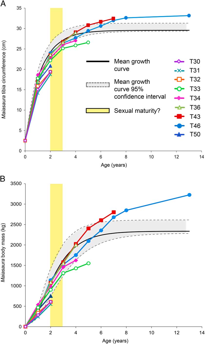
Figure 2 Growth curves for Maiasaura peeblesorum. Age in years (determined by the number of LAGs) is plotted against size: A, tibial minimum diaphyseal circumference, B, body mass. The monomolecular model was used to plot mean tibial diaphyseal circumference, whereas the von Bertalanffy model was used to plot mean body mass. Mean curves were fitted based on the five largest tibiae included in the graph; the four smaller tibiae with only two LAGs did not have enough data points to fit the models. The 95% confidence intervals are based on mean residual standard error around the mean curve, not the individual curves. Yellow bar indicates hypothesized age at which individuals would become sexually mature.
Table 3 The 95% confidence intervals around Maiasaura mean growth curve model parameters. The 95% confidence intervals were calculated using parametric bootstrapping on the mean residual standard error. Mean values are the average of values for the five tibiae with three or more LAGs (T33, T34, T36, T43, and T46). Abbreviations: m, shape parameter; A, asymptotic size in units listed in the Dataset column; K, relative growth rate per year; I, age in years at inflection point of growth curve. “Time to 95% Max Size” indicates the age in years at which 95% of asymptotic size is reached.
Myhrvold (Reference Myhrvold2013) suggested that many published dinosaur ontogenetic body mass curves are fraught with errors in calculations or rely on largely untested mass interpolation methods (including DME, used here). Even if this were not the case, most dinosaur body mass curves are derived from linear measurements, providing ample opportunities for volumetric scaling errors (see Lee et al. Reference Lee, Huttenlocker, Padian and Woodward2013). Also, due to the complete lack of associated skeletal elements in the Maiasaura bonebed, we must assume that tibia and femur lengths increased isometrically in order to apply the DME to femur lengths estimated from tibia lengths. A study on Maiasaura by Dilkes (Reference Dilkes2001) does suggest isometry of the hindlimb, but Kilbourne and Makovicky (Reference Kilbourne and Makovicky2010) suggest positive allometric growth. Because of the many potential sources of error, body mass curves in Figure 2B should therefore be considered with caution. Despite these caveats, the growth history of an animal is best illustrated in three dimensions and we include body mass curves here to illustrate a generalized volumetric growth trajectory for Maiasaura, and to allow comparisons with ontogenetic body mass curves published for other dinosaur species.
To complement growth curves derived from tibia and femur lengths here and elsewhere, and to circumvent the allometric versus isometric growth problem, we present a novel method to directly compare growth rate data across various taxa. Maiasaura tibia annual cross sectional cortical area growth was plotted against cumulative cross sectional cortical area and normalized by the largest skeletally mature values in the sample. This normalization results in quantifiable measurements from Maiasaura individuals plotted on a dimensionless scale from 0% to 100% maximum size, with no need for potentially erroneous body size calculations. The same method was applied to a sample of twelve Alligator mississippiensis femora of known ages: ten captive male Alligator mississippiensis femora, representing nine skeletally mature 26 and 27 year old individuals with EFS (Woodward et al. Reference Woodward, Horner and Farlow2011) and one immature individual at least eight years of age; and two immature 5 year olds, one of which does preserve the first LAG, yielding size at age 1 year (Woodward et al. Reference Woodward, Horner and Farlow2014). A perinate Alligator femur was also measured to provide femur size at hatching. Because cortical measurements are normalized, the Alligator and Maiasaura data could be plotted on the same graph and comparisons of annual cortical thicknesses made (Fig. 3). The innermost LAGs of the skeletally mature alligators had been destroyed by medullary expansion, so that the first data point for each line is not that of the first LAG but instead marks an average of approximately the seventh year of growth. Because the growth marks within an EFS are so closely spaced, accurately measuring the annual cortical growth is extremely difficult, so the cortical area within the entire EFS was divided by the number of growth marks, yielding equal annual growth for each year represented by the EFS. Although no alligator tibiae were available for comparison, results from Woodward et al. (Reference Woodward, Horner and Farlow2014) demonstrate that Alligator mississippiensis femur cortical thickness increases are comparable to tibia cortical thickness increases, and that the femur and tibia are amongst the fastest growing alligator limb elements. In turn, Farlow et al. (Reference Farlow, Hurlburt, Elsey, Britton and Langston2005) show that Alligator femoral dimensions including midshaft circumference can be used to predict total length. The dataset from Farlow et al. (Reference Farlow, Hurlburt, Elsey, Britton and Langston2005) also reveal a tight correlation between femoral midshaft cortical area and body mass (Supplementary Figure 3). Although Maiasaura and Alligator have very different body plans and ontogenetic limb allometries, tibiae and femora are still amongst the fastest growing elements in both taxa and reliably reflect body size increases. Regardless, our method must still be used with caution as it is susceptible to differing allometries across taxa, but it may be used to complement body mass curves by offering another way to compare growth in different taxa.

Figure 3 Annual growth of cross sectional cortical area in Maiasaura and Alligator. The y-axis represents the increase in cross sectional cortical area over a single year t, and the x-axis represents the total cross sectional cortical area at year t. Both axes are normalized so that the cross sectional cortical area at death of the largest sampled individual for each taxon equals 1. The LAG age of each Maiasaura data point is indicated next to its triangle. Individuals that died during their first growth hiatus are indicated by open triangles. The only Alligator specimen to preserve the first LAG has the LAG number of each data point indicated next to its circle. Maiasaura have the greatest cortical area growth in their first year, with annual growth steadily decreasing; 95% of growth is completed by 7 to 8 years of age. Alligator have a proportionally slower, steadier growth of cortical area. All but three Alligator specimens were 26 to 27 years of age at time of death; the largest individual completed 95% of its growth by 23 to 24 years of age. The spread of lines for each taxon demonstrates individual variation in body size and growth rate. If an individual had an EFS, this is indicated on the graph by a horizontal series of equally spaced points. The locations of the Alligator EFS segments along the x-axis demonstrate individual variation in asymptotic body size relative to the largest specimen.
Results
Predicting Maiasaura tibia medullary cavity circumference and area from tibia length (or vice versa) is not reliable (R2=0.79), indicating some variability in medullary cavity values associated with similar tibia lengths (Supplementary Tables 5–6). There is, however, a strong linear relationship between tibia length and diaphyseal circumference (R2=0.95; y=0.3685x−0.2654) (Supplementary Table 4), and a strong exponential relationship between tibia length and total cortical area (R2=0.96; y=3.5948e 0.0335x) (Supplementary Table 7), as well as tibia length and diaphyseal bone wall thickness (R2=0.97; y=3.8309e 0.0309x) (Supplementary Table 8).
Throughout ontogeny, the diaphyseal cortex is made of well vascularized woven fibered tissue (Fig. 4A). Only in the outermost cortex of the largest tibiae in the sample does vascularity decrease and tissue fiber become organized in parallel (Fig. 4E). As observed by Horner et al. (Reference Horner, de Ricqlès and Padian2000), the vascular pattern found in young tibiae (up to LAG 2) is largely a mix of laminar and reticular, becoming increasingly sub plexiform to plexiform after the second LAG. We also confirm the observations of Horner et al. (Reference Horner, de Ricqlès and Padian2000) that vascular organization changes frequently about the cortex. Secondary osteon density within the cortex is minimal throughout the sample. Rather, multiple generations of secondary osteons are found in a narrow, radial strip or “anterolateral plug” (sensu Hübner Reference Hübner2012) from innermost cortex to the periosteal surface near the anterior tibial border in larger tibiae. These secondary osteons are located in larger tibiae where a column of radial vascularity exists in smaller tibiae, and both the radial primary tissue as well as the remodeled secondary tissue “plug” is most likely related to a tendonous insertion near the anterior tibial border.
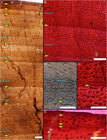
Figure 4 Vascular cyclicity, LAGs, and an external fundamental system (EFS) from the diaphyseal midshaft of Maiasaura tibia T46. A, Lateral radial transect from inner cortex (bottom) to the periosteal surface (top). The lowermost arrow indicates LAG 2. Dotted lines mark the shift from predominately reticular vascularity immediately following a LAG (arrow) to laminar or plexiform vascularity prior to the subsequent LAG. Polarized light. Scale bar, 1mm. B, The mid cortex of (A) at higher magnification detailing the cyclical change in vascularity (dotted lines) within the zones bounded by LAGs 3 and 4 (arrows). 540 nm wave plate. Scale bar, 1 mm. C, Cortical microstructure from a red deer (Cervus elaphus) (image courtesy of M. Köhler) showing a LAG (arrow) as well as a zonal transition (dotted line) in vascular organization, similar to what is observed in Maiasaura. Scale bar, 500 μm. D, LAGs (arrow) in Maiasaura tibiae are very thin and easily overlooked. 540 nm wave plate. Scale bar, 500 μm. E, The EFS (arrows) at the periosteal surface showing three closely spaced LAGs within an organized matrix and longitudinal vascular canals. 540 nm wave plate. Scale bar, 500 μm.
The rapidly deposited, woven fibered cortical matrix of Maiasaura tibiae examined in this study often contains lines of arrested growth (LAGs; Fig. 4). Much like rings within a tree trunk, LAGs indicate annual pauses in appositional growth (e.g., Peabody Reference Peabody1961; Köhler et al. Reference Köhler, Marin-Moratalla, Jordana and Aanes2012), allowing the ageing of Maiasaura individuals. The LAGs in Maiasaura tibiae are identified as thin black lines within the primary cortical tissue. Unless obfuscated by secondary remodeling or missing/damaged cortex, LAGs are fully traceable about the circumference of the section, are parallel to each other, and in general become more closely spaced near the outer cortex of larger individuals.
Tibia lengths for individuals approaching one year of age range between 29.4 cm and 48.8 cm (Fig. 1), with diaphyseal circumferences 14.3–18.3 cm. Size variation continues throughout ontogeny, with tibia lengths between 56–69.5 cm and corresponding diaphyseal circumferences of 21.4–26.5 cm by the third year of life. Tibia length (75–88 cm) and circumference (28–33 cm) begin to plateau between the sixth and eighth year of life. No tibiae 49–55.5 cm in length or 70–75 cm in length are present in the sample. In the largest tibiae, medullary expansion and secondary osteons only partially destroy the first LAG.
At low magnification (10× total) even the cortices of some of the smallest tibiae examined (33.8–48.8 cm in length) appear to have LAGs. But close examination at higher magnification (40× to 100× total magnification) reveals concentric bands of localized changes in the diameter and orientation of vascular canals (Fig. 5). True LAGs first appear in thin sections from tibiae 56 cm in length and larger (Fig. 4), but no tibiae in the sample possess only a single LAG and tibiae with only three LAGs are also absent. Specimens 56–69.5 cm in length all possess two LAGs and those 75–99.7 cm in length have between four and ten LAGs (Fig. 1, Supplementary Table 1). The tibiae 75 cm in length and larger also have progressively more closely spaced LAGs nearing the periosteal surface, with five tibiae being skeletally mature as revealed by the presence of an external fundamental system (EFS). By utilizing the regression equation resulting from plotting tibia length against diaphyseal circumference (y=0.3685x−0.2654), the first (innermost) LAG circumference measurements from tibiae 56 cm in length and greater reveal lengths between 39 cm and 51 cm at the close of the first year of growth (Supplementary Table 2).
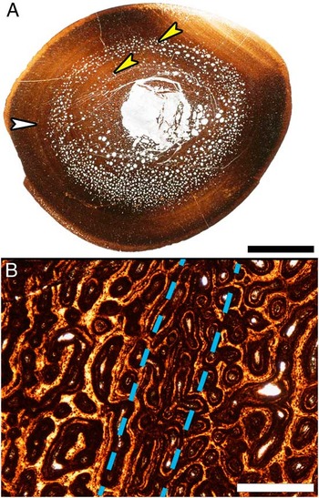
Figure 5 Resorption cavity rings and localized vascular changes within the cortex of a Maiasaura tibia (T16) approaching one year of age. A, Mid diaphyseal transverse section with two resorption cavity rings (yellow arrows) within the cortex. The white arrow indicates a ring within the cortex that could be mistaken for a line of arrested growth (LAG). Scale bar, 1 cm. B, Enlargement of the region indicated by the white arrow in (A), centered on the ring visible within the cortex (between dashed lines). At this magnification it becomes apparent that the ring is formed by a localized change in vascular canal size and that no LAG is present. Scale bar, 500 μm.
Based on the complete absence of LAGs, 31 tibiae within the sample set represent individuals less than one year of age. Thus, Maiasaura young of the year mortality rate is high (≥89.9%). After the first year, mortality rate sharply decreases (Fig. 6). There is a brief increase in mortality rate between years 2 and 3. By dividing the non juvenile (i.e., 2 or more years of age) Maiasaura into two age groups, the mortality rates of those age groups can be compared. The non juvenile age groupings with the greatest difference in mortality rates (and smallest 95% confidence interval) are 2–8 years old (mean annual mortality rate 12.7%) compared with 9–15 years old (mean annual mortality rate 44.4%), indicating that a second period of elevated mortality begins between 8 and 9 years of age.

Figure 6 Survivorship curve for Maiasaura. Sample size of 50 tibiae was standardized to an initial cohort of 1000 individuals (assumes 0% neonate mortality). Survivorship is based on the number of individuals surviving to reach age x (the end of the growth hiatus marked by LAG x). Age at death for individuals over 1 year old was determined by the number of LAGs plus growth marks within the EFS, when present. Error bars represent 95% confidence interval. Mean annual mortality rates ( $\hat{\mu }$
) given for age ranges 0–1 years, 2–8 years, and 9–15 years. Vertical gray bars visually separate the three mortality rate age ranges.
$\hat{\mu }$
) given for age ranges 0–1 years, 2–8 years, and 9–15 years. Vertical gray bars visually separate the three mortality rate age ranges.
A large portion of early rapid growth was achieved during the first year, with bone apposition rate averaging 65.1 μm/day, decreasing to 21.4 μm/day in the second year, and falling again in the third year to 13.7 μm/day (Table 1). By the ninth year, average apposition rate declines to 2.6 μm/day. Despite annual apposition rate reductions, in the zones of cortex separated by LAGs, fiber orientation is woven and the tissue is well vascularized throughout most of ontogeny (Fig. 4A). Reticular, sub laminar, and laminar vascularity predominates in smaller tibiae (<70 cm in length), and a greater proportion of laminar and plexiform vascularity occurs in larger specimens (>70 cm in length). However, even when observing similar locations around the cortex, vascular canal orientation differs among same size tibiae as well as ontogenetically.
Within the woven fibered zones of the cortex, two peculiar patterns of resorption and vascularity present themselves. The first are concentric resorption cavity rings in the mid cortex of tibiae between 40 cm and 50 cm in length (i.e., young of the year) (Fig. 5A). The second unusual vascular arrangement begins in larger tibiae: immediately following the second LAG, vascular canals are initially reticular corresponding to high apposition rates (average 31.6–33.2 μm/day in ratites (Castanet et al. Reference Castanet, Rogers, Cubo and Boisard2000)). Then the vascular pattern transitions to laminar or plexiform with somewhat lower apposition rates (average 24.7–27.1 μm/day in ratites (Castanet et al. Reference Castanet, Grandin, Abourachid and de Ricqlès1996; Castanet et al. Reference Castanet, Rogers, Cubo and Boisard2000)) for the majority of the zone (Fig. 4A, B). The progression from reticular to dominantly laminar or plexiform then repeats within each successive zone, but becomes less prevalent in the more closely spaced zones immediately prior to the EFS. This repeating vascular pattern is consistently seen in posterior orientation of the cortex, and may be less pronounced or even absent at other locations about the transverse section.
For modeling tibia circumference and body mass curves, the monomolecular model was the best fit (lowest mean AICc) for the former, and the von Bertalanffy model was the best fit for the latter (Table 2). Figure 2A and 2B plot the circumference and mass curves (respectively) for each of the nine individuals for which enough LAGs were preserved, but only the five largest tibiae of the nine were used to model the mean growth curves. Individual tibiae display a range of individual body size variation; the mean curve represents the mean of the model curves fit to each of the individual tibiae. The difference between the fit of each model curve and the actual individual data points is represented by the residual standard error. The mean of the residual standard error was used to construct the 95% confidence intervals around the mean curve (see Methods). Thus, the 95% confidence intervals represent a range of variation around the mean line that would contain 95% of data points if the mean line were constructed from an actual tibia instead of an idealized perfect curve model. Individual body sizes may be smaller or larger than this mean curve and its confidence intervals; the growth trajectory of a smaller bodied individual would resemble a slightly scaled down version of the mean curve and confidence intervals, and a larger bodied individual would resemble a slightly scaled up version.
According to the mean growth curve model, mean body mass and tibia diaphyseal circumference at the close of the first year of growth is 384.3 kg and 17.4 cm respectively, and increases to 1632 kg and 27.1 cm by the end of the third year of growth (LAG 3). Growth begins to plateau after LAG 8 as the mean asymptotic body mass of 2337.4 kg and tibia circumference of 29.6 cm is approached.
Discussion
Cyclical Growth Marks
The diaphyseal cortices of tibiae 33.8–48.8 cm in length appear to possess LAGs. However, examinations at higher magnifications reveals that these structures are instead concentric rings of localized changes in vascular canal orientation and diameter (Fig. 5), and were previously described in Maiasaura elements categorized as juvenile by Horner et al. (Reference Horner, de Ricqlès and Padian2000). We agree with the original conclusion that such localized vascular fluctuations are the result of changes in bone apposition rate and not of arrested growth, and that more research on extant bone tissue growth is needed to understand their cause before they could be interpreted as annual growth marks in very fast growing bone. On the other hand, the cortex of every tibia 56 cm in length and larger contains true LAGs. Even at tibia lengths of 75 cm and greater, continued medullary expansion and frequent secondary osteons only partly destroy the innermost LAG. Calculated tibia lengths corresponding to the circumference of the first (innermost) LAG in tibiae 56 cm or larger are between 39 cm and 51 cm (Supplementary Table 2). A LAG becomes visible after growth resumes, so specimens from the sample without LAGs, but between 39 cm and 51 cm in length, therefore represent individuals that perished while experiencing their first annual growth hiatus and illustrate the size variability already present at this young age.
The thickness of cortical zones between each LAG represents yearly bone apposition that, in the Maiasaura tibia cortices, progressively decreases with increasing age. Reduction in yearly cortical apposition (and therefore growth rate) is especially apparent in tibiae 75 cm in length or greater (>7 LAGs), and such pronounced reduction is associated with nearing skeletal maturity.
By retro calculating missing LAGs to construct a growth history, and also by using experimentally obtained growth rate estimates for various limb bone types in extant taxa, Horner et al. (Reference Horner, de Ricqlès and Padian2000) estimated that Maiasaura attained skeletal maturity in six to eight years. Of the eleven tibiae in our sample with at least 7 LAGs, five (45.4%) possess an external fundamental system (EFS) in the outermost cortex (Fig. 4E). In extant vertebrates, the EFS is associated with attainment of skeletal maturity as it signals the effective cessation of long bone increase in length (Cormack Reference Cormack1987; Castanet et al. Reference Castanet, Newman and Girons1988). The mean age at which skeletal maturity occurred in the five individuals with EFS is 8.25 years, which supports the original estimate of six to eight years by Horner et al. (Reference Horner, de Ricqlès and Padian2000). The remaining six tibiae with at least 7 LAGs (54.5%) are a mean age of 8.7 years but lack an EFS, revealing individual variation not only for the age at which skeletal maturity occurs, but also in corresponding tibia lengths at skeletal maturity. For instance, two tibiae, both with 8 LAGs prior to their EFS, have respective tibia lengths of 75 cm and 87.5 cm. But a third tibia 90 cm in length has 10 LAGs and no EFS, indicating that at ten years of age this individual was still growing. Further variability in age and tibia length at skeletal maturity will likely manifest as additional large specimens are incorporated into the sample.
Survivorship, Maturity, and Longevity
Dinosaur population survivorship has been previously modeled for Albertosaurus, Gorgosaurus, Daspletosaurus, Tyrannosaurus, and Psittacosaurus (Erickson et al. Reference Erickson, Currie, Inouye and Winn2006; Erickson et al. Reference Erickson, Makovicky, Inouye, Zhou and Gao2009; Erickson et al. Reference Erickson, Currie, Inouye and Winn2010). Unfortunately, due to the difficulty presented by fossil scarcity and in obtaining multiple specimens for histological sampling, such modeling has been criticized for its lack of biologically statistically significant sample sizes (Steinsaltz and Orzack Reference Steinsaltz and Orzack2011). The minimum number of specimens required to construct meaningful survivorship curves was suggested as 50 in a critique of Albertosaurus survivorship curves by Steinsaltz and Orzack (Reference Steinsaltz and Orzack2011). Although far from the hundreds or thousands of individuals comprising modern vertebrate and invertebrate survivorship studies, the 50 Maiasaura tibiae of known (rather than estimated) age utilized in our sample is the largest yet for any dinosaur taxon; meets the minimum sample number advocated by Steinsaltz and Orzack (Reference Steinsaltz and Orzack2011) for survivorship studies; and is the first to incorporate an entire ontogenetic series from hatching to skeletal maturity with no age estimation or retro calculation. It is important to note, however, that our Maiasaura sample set is highly atypical for fossil taxa (especially dinosaurs). Due to the likelihood of fossil tetrapod preservation, paleontologists are commonly restricted to small numbers of fossils for any kind of research. Thus, a prerequisite of at least 50 fossil specimens for population analyses is unreasonable for most extinct tetrapod taxa. When viewed in this way, the Maiasaura sample is a fortunate exception, providing valuable insights into the population biology of an extinct animal.
Varricchio and Horner (Reference Varricchio and Horner1993) reported a skeletal element length frequency distribution for the Maiasaura bonebed that included humeri (n=20), tibiae (n=16), and femora (n=18). Based on size distribution, they concluded there was high juvenile mortality and predicted that the majority of the sample was made of young of the year. Our age frequency distribution of Maiasaura also suggests age specific mortality biased towards the very young as well as senescent attrition, rather than representing an accurate profile of the living population structure (Fig. 1) (Voorhies Reference Voorhies1969; Varricchio and Horner Reference Varricchio and Horner1993; Erickson et al. Reference Erickson, Currie, Inouye and Winn2010). The combination of Maiasaura high initial mortality followed by a period of low mortality, and eventually ending in senescent attrition, closely resembles the sigmoidal B1 type survivorship curve (Pearl and Miner Reference Pearl and Miner1935), which is frequently associated with a survivorship study by Deevey (Reference Deevey1947) on Dall sheep (Ovis dalli). Although the B1 survivorship pattern has been suggested for other dinosaur groups (Albertosaurus, Gorgosaurus, Daspletosaurus, Tyrannosaurus, and Psittacosaurus; Erickson 2006; 2009), ours is the first study to demonstrate this B1 pattern utilizing individuals ranging from hatching and less than one year of age through skeletal maturity, with no retrocalculations or estimations of age.
A modern analogue to Maiasaura survivorship presents itself in a red deer (Cervus elaphus) population from the Isle of Rum, Scotland. Of the many ongoing mammal and bird population studies, we chose to use the Isle of Rum red deer as analogues for interpreting Maiasaura survivorship patterns due to the data available to support the red deer ecological interpretations: The Isle of Rum Red Deer Project (http://rumdeer.biology.ed.ac.uk/) is one of the longest running (since 1953) scientific studies of a vertebrate population in the world. Over sixty years of research on this population results in detailed studies on pedigree, behavior, life history trade offs, and survivorship. In addition to the accumulated Isle of Rum data, red deer are acceptable analogues because of the similarities not only between Maiasaura and red deer survivorship curve type (B1), but also in bone tissue organization: woven bone tissue separated by growth marks in both taxa indicates high sustained growth rates occurring over a period of years (Fig. 4C); furthermore, both taxa are relatively large bodied quadrupedal herbivores.
Thirty one of the fifty Maiasaura tibiae examined here lack LAGs, meaning that young of the year make up over half of our sample (Fig. 1). This signal is also reflected in the frequency distribution of Maiasaura femora from the bonebed, as 13 of the 18 femora (72%) included in a limb frequency analysis by Varricchio and Horner (Reference Varricchio and Horner1993) were less than 50 cm in length, and femora of this length represent young of the year according to the analysis by Horner et al. (Reference Horner, de Ricqlès and Padian2000). The corresponding mean mortality rate for the first year of growth based on the tibiae in our sample is at least 89.9%. After the first year of life the mean mortality rate falls to 12.7% (Fig. 6). For the red deer population, juvenile mortality is highest during the first two winters after weaning, when the animals may succumb to the high energy costs of rapid growth during a period of reduced resources (Clutton-Brock et al. Reference Clutton-Brock, Albon and Guinness1985; Catchpole et al. Reference Catchpole, Fan, Morgan, Clutton-Brock and Coulson2004). In extant alligators as well as ruminants such as the red deer, the annual growth hiatus occurs during unfavorable months when resources are less plentiful (Joanen and McNease Reference Joanen and McNease1987; Köhler et al. Reference Köhler, Marin-Moratalla, Jordana and Aanes2012). Perhaps the annual Maiasaura growth hiatus also corresponded to a seasonally stressful period, during which time the young of the year were particularly susceptible to predation, starvation, exposure to weather, or other external factors, increasing the mortality rate for this age group.
In contrast to the high number of early juveniles present in the Maiasaura sample, those between one and two years of age (yearlings) are absent (Fig. 1). In other words, no tibiae possess only a single LAG. Horner et al. (Reference Horner, de Ricqlès and Padian2000) found the same to be true of the six femora included in their Maiasaura ontogenetic histologic analysis: the “late juvenile” category femur (50 cm in length) lacked LAGs, and the next largest (68 cm) already had two LAGs. That the absence of individuals between one and two years of age is recorded in both femora and tibiae adds support to our hypothesis that yearlings were rarely incorporated into the bonebed. Thus, it seems that if young Maiasaura could endure their first unfavorable season, the chances of surviving another year were high. A slight increase in mortality occurred between 2 and 3 years of age (2 LAGs), which may signal attainment of sexual maturity (Erickson et al. Reference Erickson, Currie, Inouye and Winn2006, Reference Erickson, Currie, Inouye and Winn2010) and the accompanying increased physiological demands related to breeding and/or competition for mates (Fig. 6). The complete absence of three and four year olds (3–4 LAGs; Fig. 1) from the sample suggests that individuals able to withstand the onset of this additional stress would likely live into their fifth year before mortality began to rise again, which is reflected in the mean mortality rate of only 12.7% for Maiasaura between 2 and 8 years of age (Fig. 6). Such a mortality plateau is also exhibited by the Isle of Rum red deer. For red deer, this period begins around the third year of life coinciding with sexual maturity onset and marks a time of peak performance, when survival and reproductive success are highest (Catchpole et al. Reference Catchpole, Fan, Morgan, Clutton-Brock and Coulson2004; Nussey et al. Reference Nussey, Kruuk, Morris, Clements, Pemberton and Clutton-Brock2009).
A second period of elevated mortality in Maiasaura begins between eight and nine years of age (44.4% mean annual mortality rate; Fig. 6). The mortality rate of Isle of Rum red deer also rises between eight and nine years of age, as they enter a period of senescence, defined by Jones et al. (Reference Jones, Gaillard, Tuljapurkar, Alho, Armitage, Becker, Bize, Brommer, Charmantier, Charpentier, Clutton-Brock, Dobson, Festa-Bianchet, Gustafsson, Jensen, Jones, Lillandt, McCleery, Merila, Neuhaus, Nicoll, Norris, Oli, Pemberton, Pietiainen, Ringsby, Roulin, Saether, Setchell, Sheldon, Thompson, Weimerskirch, Jean Wickings and Coulson2008) as “a decline in fitness with age caused by physiological degradation” (p. 665). For Maiasaura, eight years coincides with mean age at skeletal maturity, supporting a senescence correlated increase in mortality.
The B1 survivorship pattern observed in Maiasaura – presumed high juvenile mortality, followed by a mortality plateau, and lastly elevated adult mortality – was previously reported for the basal ceratopsid Psittacosaurus (Erickson et al. Reference Erickson, Makovicky, Inouye, Zhou and Gao2009) and for the tyrannosaurid Albertosaurus (Erickson et al. Reference Erickson, Currie, Inouye and Winn2006, Reference Erickson, Currie, Inouye and Winn2010). The same B1 pattern recorded in the Isle of Rum red deer population was used to support the antagonistic pleiotropy theory of ageing, which states that achieving sexual maturity early in life reduces reproductive performance and survival probabilities later in life (Nussey et al. Reference Nussey, Wilson, Morris, Pemberton, Clutton-Brock and Kruuk2008). Red deer studies also suggest that the magnitude of senescence is directly related to early development; essentially, animals that achieve peak performance early, senesce quickly (Jones et al. Reference Jones, Gaillard, Tuljapurkar, Alho, Armitage, Becker, Bize, Brommer, Charmantier, Charpentier, Clutton-Brock, Dobson, Festa-Bianchet, Gustafsson, Jensen, Jones, Lillandt, McCleery, Merila, Neuhaus, Nicoll, Norris, Oli, Pemberton, Pietiainen, Ringsby, Roulin, Saether, Setchell, Sheldon, Thompson, Weimerskirch, Jean Wickings and Coulson2008). These hypotheses explain the survivorship curves exhibited by Maiasaura, Psittacosaurus, and Albertosaurus: the dinosaurs grew rapidly to attain the minimum body size necessary to escape strong environmental and predatory pressures (Cooper et al. Reference Cooper, Lee, Taper and Horner2008), and achieved peak performance relatively early in ontogeny (sensu Albon et al. Reference Albon, Clutton-Brock and Guinness1987). The consequence for high energy demands early in ontogeny is high juvenile mortality followed by rapid senescence after the peak performance window (Jones et al. Reference Jones, Gaillard, Tuljapurkar, Alho, Armitage, Becker, Bize, Brommer, Charmantier, Charpentier, Clutton-Brock, Dobson, Festa-Bianchet, Gustafsson, Jensen, Jones, Lillandt, McCleery, Merila, Neuhaus, Nicoll, Norris, Oli, Pemberton, Pietiainen, Ringsby, Roulin, Saether, Setchell, Sheldon, Thompson, Weimerskirch, Jean Wickings and Coulson2008). If proportionally few dinosaurs in a population survived beyond the onset of sexual maturity (only 28% in our Maiasaura sample), and mortality related to senescence rose immediately following the peak performance plateau, this may explain why exceptionally large, skeletally mature dinosaurs with thick EFS are rare in the fossil record (e.g., Erickson Reference Erickson2005; Erickson et al. Reference Erickson, Currie, Inouye and Winn2006; Erickson et al. Reference Erickson, Makovicky, Inouye, Zhou and Gao2009; Horner et al. Reference Horner, Goodwin and Myhrvold2011).
Apposition Rates and Ontogenetic Growth
The bone apposition rate in Maiasaura was highest during the first year of life, with a mean of 65.1 μm/day, falling to 13.7 μm/day by the third year of life and presumed onset of sexual maturity (Table 1). Continued body size increase likely remained advantageous after reaching sexual maturity, but proceeded at lower rates approaching an asymptote; average apposition rate declined annually to 2.6 μm/day by year nine. Although apposition rate steadily declined over ontogeny, woven bone continues to be deposited until skeletal maturity was achieved (Fig. 4). Vascular orientation did change throughout ontogeny, with reticular, sub laminar, and laminar vascularity common in smaller tibiae (<70 cm in length), and increased amounts of laminar and plexiform vascularity in larger specimens (>70 cm in length). Differences in vascular orientation about the cortex within a woven fibered matrix may indicate either changes in mechanical loading (de Margerie et al. Reference de Margerie, Cubo and Castanet2002) or apposition rates (de Margerie et al. Reference de Margerie, Robin, Verrier, Cubo, Groscolas and Castanet2004), although the two are not mutually exclusive. Regardless, the variability in vascular arrangement among the smallest specimens, combined with a cyclically repeating vascular pattern observed within zones of older individuals (see below), shows that in Maiasaura ontogenetic vascularity changes were influenced most strongly by growth rate fluctuations.
Among extant archosaurs, woven fibered tissue is only extensively present in Aves, where apposition rates range between 5 μm/day to 171 μm/day, but with considerable overlap in rates for different vascular arrangements (Castanet et al. Reference Castanet, Grandin, Abourachid and de Ricqlès1996; Castanet et al. Reference Castanet, Rogers, Cubo and Boisard2000; de Margerie Reference de Margerie2002; de Margerie et al. Reference de Margerie, Cubo and Castanet2002; Starck and Chinsamy Reference Starck and Chinsamy2002; de Margerie et al. Reference de Margerie, Robin, Verrier, Cubo, Groscolas and Castanet2004). For instance, avian histology studies report that, depending on species and skeletal element, the range of average apposition rates are between 10 μm/day and 39.5 μm/day for reticular, laminar, sub laminar, and sub plexiform vascularity (Castanet et al. Reference Castanet, Grandin, Abourachid and de Ricqlès1996; Castanet et al. Reference Castanet, Rogers, Cubo and Boisard2000); 4.8–50 μm/day for longitudinal vascularity (Castanet et al. Reference Castanet, Rogers, Cubo and Boisard2000; Starck and Chinsamy Reference Starck and Chinsamy2002); and 5–15 μm/day for plexiform (Castanet et al. Reference Castanet, Grandin, Abourachid and de Ricqlès1996). Density of vessels decreases below a rate of 5 μm/day, and below 1 μm/day vascularity disappears and parallel fibered tissue dominates (Castanet et al. Reference Castanet, Grandin, Abourachid and de Ricqlès1996). After the fifth year of life Maiasaura average apposition rates generally fall below 3 μm/day within the realm of decreased vascularity and parallel fibered organization. These rates are counterintuitive since qualitative observation shows cortical tissue remains consistently well vascularized and woven for several additional zones prior to the EFS (Fig. 4). Somewhat higher average annual apposition rates result by incorporating the growth hiatus into apposition estimates. This method has not previously been applied to dinosaurs, but can be demonstrated using extant taxa (Joanen and McNease Reference Joanen and McNease1987; Castanet et al. Reference Castanet, Newman and Girons1988). For instance, the growing season for alligators in Louisiana is approximately seven months (Joanen and McNease Reference Joanen and McNease1987) and so their average annual apposition rates should be based on a growing season of 214 days rather than 365 days. The duration of the growth hiatus in Maiasaura is unknown, but we conservatively estimate a minimum of three months as determined for extant ruminants (Köhler et al. Reference Köhler, Marin-Moratalla, Jordana and Aanes2012). A comparison beyond the archosaurian extant phylogenetic bracket is justified here as ruminant bone microstructure consists of rapidly growing tissue separated by LAGs (Fig. 4C), therefore resembling Maiasaura tissue organization more closely than that of either crocodylians (no extensive woven tissue) or birds (most take less than a year to reach skeletal maturity (Castanet Reference Castanet2006)). Using this approach, the average daily apposition rate of Maiasaura prior to the first hiatus was 86.4 μm/day; 28.4 μm/day for yearlings; 18.2 μm/day during the third year; and falling to 3.5 μm/day by the ninth year (Table 1). These adjusted apposition rates consider the yearly growth hiatus and remain within the recorded range for woven, well vascularized avian tissues for most of ontogeny, while also tracking the decrease in vascularity occurring in the zones immediately preceding the EFS in the largest specimens.
The vertebrate growth hiatus is still not fully understood, requiring further research on extant vertebrates. A novel approach is to explore whether growth hiatus duration lengthens with increasing age, since duration changes by latitude and with photoperiod manipulation (Joanen and McNease Reference Joanen and McNease1987; Lance Reference Lance1989; Wilkinson and Rhodes Reference Wilkinson and Rhodes1997; Castanet et al. Reference Castanet, Croci, Aujard, Perret, Cubo and de Margerie2004). If yearly apposition rate was constant while the growth hiatus increased during Maiasaura ontogeny, the high first year apposition rates (57.0–100.9 μm/day) could be sustained throughout growth (Table 1). These rates are well within the range observed in extant Aves, while offering a novel alternative hypothesis to explain how tissue organization remained woven throughout ontogeny even as zone thickness progressively decreased. Actual Maiasaura growth may have combined a decrease in apposition rate with an increase in duration of the growth hiatus, thus falling between the extremes bracketed in Table 1.
Comparative Analysis of Apposition Rates
The appositional growth rate data acquired from Maiasaura are useful not only for a deeper understanding of its growth history, but also for growth rate comparisons across taxa. As an example, normalized Maiasaura tibia cortical growth was plotted alongside normalized Alligator mississippiensis femur cortical growth (Fig. 3), with the simple purpose of testing the hypothesis that the growth histories of these two archosaur taxon will exhibit marked differences when directly compared in a normalized fashion. Alligators are a very well studied group histologically, and are often utilized to understand zonal bone growth in dinosaurs (e.g., Erickson Reference Erickson1996; Farlow and Britton Reference Farlow and Britton2000; Farlow et al. Reference Farlow, Hurlburt, Elsey, Britton and Langston2005; Schweitzer et al. Reference Schweitzer, Elsey, Dacke, Horner and Lamm2007; Tumarkin-Deratzian Reference Tumarkin-Deratzian2007; Tumarkin-Deratzian et al. Reference Tumarkin-Deratzian, Vann and Dodson2007; Klein et al. Reference Klein, Scheyer and Tütken2009; Farmer and Sanders Reference Farmer and Sanders2010; Woodward et al. Reference Woodward, Horner and Farlow2011, Reference Woodward, Horner and Farlow2014). The seemingly obvious comparison of dinosaur histology to that of their extant bird descendants does not apply here, because (with few exceptions), extant birds achieve adult size in less than a year and therefore do not deposit zonal bone. The 12 alligators used in this comparison were captive raised and therefore possessed growth rates much higher than their wild counterparts, and the nine oldest specimens had in fact attained skeletal maturity before their 26th year of life (Woodward et al. Reference Woodward, Horner and Farlow2011). Unfortunately, Alligator tibia data were not available to compare directly to Maiasaura tibia data. However, Woodward et al. (Reference Woodward, Horner and Farlow2014) demonstrate that out of the appendicular elements examined, the femur and tibia have the highest annual increase in cortical area for the alligators studied, with the femur exceeding that of the tibia. Therefore, alligator femur cortical area increase likely provides an overestimate of alligator tibia cortical area increase. In addition, Alligator mississippiensis femoral dimensions are demonstrated to tightly correlate with body length and body mass (Supplementary Figure 3; Fig. 2 and Fig. 3 in Farlow et al. Reference Farlow, Hurlburt, Elsey, Britton and Langston2005); alligators are well studied and the histological dataset utilized consists of animals of known age, weight, body length, and sex; and alligators are one of the few extant archosaurs approaching the body size of a hadrosaur.
Normalized comparison demonstrates that Maiasaura annual cortical increase was highest in the youngest specimens and steadily decreased over ontogeny, but admittedly, the extent to which an ontogenetic transition from bipedal to quadrupedal posture in Maiasaura (Dilkes Reference Dilkes2001) may affect gait and therefore tibia bone apposition rate is currently unknown. In contrast, even using the femur, alligator cortical growth was much lower, protracted, and more or less constant throughout ontogeny, never approaching the highest rates observed for Maiasaura. Because data are normalized, hypotheses for the differences in growth rates observed can then be proposed and tested, such as differences in metabolism, gait, or ecologies.
This normalization method must be applied cautiously, as comparing different skeletal elements from taxa with different limb allometries, gaits, and ecologies can lead to erroneous conclusions about growth (see Zhao et al. Reference Zhao, Benton, Sullivan, Sander and Xu2013; Cullen et al. Reference Cullen, Evans, Ryan, Currie and Kobayashi2014). Tight correlations with limb element dimensions and body length/mass, as well as maximum appositional growth rates, as noted with the alligator femora, must be demonstrated before being utilized in such normalized comparisons to ensure that the same growth characteristics are being compared. If such conditions are demonstrated, normalized growth comparisons can complement more traditional body mass growth curve modeling. Our evaluation demonstrates two completely different growth histories in related taxa possessing LAGs and provides further evidence that the presence of LAGs is unrelated to metabolism or growth rate, and is likely a plesiomorphic characteristic retained by most, if not all, vertebrate groups (e.g., de Ricqlès et al. Reference de Ricqlès, Padian, Knoll and Horner2008).
Physiological Clues in Cortical Features
Concentric resorption cavity rings (Fig. 5) are observed in the mid cortex of some Maiasaura tibiae between 40 cm and 50 cm in length in addition to the typical random scattering of resorption cavities within the innermost cortex. These resorption rings are only found in Maiasaura tibiae representing young of the year, and closely resemble structures reported in the humerus of an immature specimen of the sauropod Alamosaurus (Woodward and Lehman Reference Woodward and Lehman2009). Resorption rings may therefore be a characteristic of young fast growing dinosaur long bones, but only for a brief time. The small sample sizes of most dinosaur histology studies reduce the likelihood of sampling this ontogenetic period, so it is unsurprising this resorption pattern has gone largely unreported in other taxa. Such a concentric arrangement of resorption cavities, rather than the more typical centripetal resorption cavity radiation, may explain how medullary expansion kept pace with the high cortical apposition rates determined here for the very young.
In all Maiasaura tibiae with more than two LAGs, a zonal vascular pattern consisting of reticular vascularity followed by laminar or plexiform vascularity appears in the cortical zone representing the third year of life and repeats until approaching skeletal maturity where the zonal spacing makes it difficult to observe (Fig. 4). A similar repeating zonal vascular pattern is described in other dinosaurs (Horner et al. Reference Horner, de Ricqlès and Padian1999; Hübner Reference Hübner2012; Hedrick et al. Reference Hedrick, Tumarkin-Deratzian and Dodson2014) including the hadrosaurid Edmontosaurus (Chinsamy et al. Reference Chinsamy, Thomas, Tumarkin-Deratzian and Fiorillo2012). Alaskan specimens of Edmontosaurus were hypothesized to exhibit this vascular cyclicity in place of LAGs and in response to annually reduced nutrient access resulting from non migratory behavior and months of polar darkness (Chinsamy et al. Reference Chinsamy, Thomas, Tumarkin-Deratzian and Fiorillo2012). Maiasaura vascular cyclicity strongly resembles that of Alaskan Edmontosaurus (except that Maiasaura also preserves LAGs), but Maiasaura inhabited much lower latitudes and would have experienced more temperate conditions (Lorenz and Gavin Reference Lorenz and Gavin1984). The presence of such a vascular pattern therefore provides no evidence of perennial polar residency, and in Maiasaura this pattern is consistently only observed after the second LAG.
Rather than a response to non migratory behavior, there is evidence that such a repeating vascular pattern is associated with cyclic hormonal changes. By examining ruminant bone microstructure and recording seasonal hormonal fluctuations, Köhler et al. (Reference Köhler, Marin-Moratalla, Jordana and Aanes2012) found a correlation between increasing levels of growth hormones and increasingly vascularized woven fibered tissue, culminating with the peak of the favorable season. This was followed by low levels of growth hormones culminating in a growth hiatus of several months during the stressful season, revealed by LAGs in the bone microstructure (Köhler et al. Reference Köhler, Marin-Moratalla, Jordana and Aanes2012). Therefore the repeating vascular pattern observed in both Maiasaura and Edmontosaurus was more likely a response to hormonal changes occurring during the favorable season irrespective of elevation or latitude. Another explanation (though not exclusive) for the vascular pattern may be that it indicates a hormonal shift and seasonal reallocation of resources for breeding, egg laying, nest protection, or caring for young, although such life events are often tied to stressful or favorable seasons and may be difficult to separate histologically from environmental reactions. However, if the vascular pattern was solely related to alternating favorable and unfavorable seasons, this pattern should be observed in tissues deposited prior to the third year of growth. The abrupt and permanent switch from largely random vascularity within zones of the youngest Maiasaura to a repeating vascular pattern following the second LAG (Fig. 4) in older individuals implies the onset of an annually repeating event affecting growth rate. Based on the Maiasaura survivorship curve (Fig. 6), we hypothesized that this taxon attained sexual maturity during the third year of life. Because this vascular pattern appears in the bone tissue during the third year of life, we suggest this pattern is independent evidence of sexual maturity onset at this age. We hypothesize that with increased ontogenetic sampling of polar Edmontosaurus a similar trend of ontogenetically delayed cyclic vascularity will almost certainly be revealed.
Linear and Three Dimensional Growth
A plot of age versus minimum diaphyseal circumference (Fig. 2A) obtained from tibiae with fully traceable LAG circumferences (n=9) shows individual size variability during ontogeny. On average Maiasaura individuals achieved over half (56%, x=16.6 cm) of their estimated asymptotic tibia circumference of 29.6 cm in their first year, and circumferences varied between 14.2 cm and 18.6 cm (Supplementary Table 2). Circumferences amongst individuals in their third year of life differ by up to 5.2 cm (24% of mean size at age 2). Growth in tibia circumference begins to plateau between the sixth and eighth year of life, with skeletal maturity occurring in one of these individuals during the eighth year of life.
A high coefficient of determination value (i.e., R2>0.9) between tibia length and diaphyseal circumference allows prediction of tibia length and ultimately body mass during each year of growth as represented by LAG circumferences (Supplementary Table 4). Individual ontogenetic variability becomes especially obvious in body mass curves, since variation in linear measurements are essentially cubed in volumetric analyses (Fig. 2). As such, body mass amongst yearlings varies by 296 kg, and by 854 kg at LAG 5. Prior to this study, a single Maiasaura body mass curve has been published, constructed upon three data points (Fig. 2 of Erickson et al. Reference Erickson, Rogers and Yerby2001). The much larger ontogenetic and longitudinal sample used here allows a synthesis of multiple curves, providing a more accurate portrayal of Maiasaura growth and the variability within the species (Fig. 2B). The Maiasaura body mass curve published by Erickson et al. (Reference Erickson, Rogers and Yerby2001) shows a relative stasis in mass increase from age one (160 kg) until age four (172 kg). The authors predicted a maximum growth rate of 1042 kg/year between ages five and six. Although no demonstrably skeletally mature individuals were included in their analysis, Erickson et al. (Reference Erickson, Rogers and Yerby2001) predicted that Maiasaura reached asymptotic body mass at age 7, as was previously calculated by Horner et al. (Reference Horner, de Ricqlès and Padian2000). In contrast, our mean body mass curve suggests a maximum growth rate of 721 kg/yr (95% confidence interval 593–859 kg/yr) occurred during the second year of growth (between LAG 1 and LAG 2) and the mean body mass asymptote of 2337 kg was approached by year eight (Fig. 2B). Individual body mass curves also show a decrease in the rate of annual mass addition after the second LAG (growth of 439–765 kg/yr between LAG 2 and LAG 3, compared to growth of 116–446 kg/yr between LAG 3 and LAG 4), reflected by reduced zone spacing (e.g., Fig. 4A). Lee and Werning (Reference Lee and Werning2008) correlated the inflection point on an S shaped curve, occurring between one third and one half asymptotic mass, to the onset of sexual maturity in several dinosaur taxa. Although the inflection point in the Maiasaura mean mass growth curve occurs at 1.44 years of age, one third asymptotic body mass had not yet been attained. Instead, one third of asymptotic body mass is attained just before age 2, and one half of asymptotic body mass is reached soon after age 2 (between LAG 2 and LAG 3; Fig. 2B). The zone between LAG 2 and LAG 3 also coincides with the appearance of a repeating vascular pattern and a temporary mortality increase within the peak performance survivorship plateau, reinforcing our hypothesis that the appearance of an alternating vascular pattern and a temporary increase in mortality rate are independent indicators of sexual maturity.
Conclusions
An ontogenetic sample size of 50 Maiasaura tibiae, representing a minimum of 32 individuals, confirmed previously published observations (Varricchio and Horner Reference Varricchio and Horner1993; Horner et al. Reference Horner, de Ricqlès and Padian2000), permitted the largest extinct tetrapod population osteohistology synthesis to date, and revealed aspects of Maiasaura growth and behavior in unprecedented detail. Our tibia series included individuals less than a year of age up to skeletal maturity and provided not only a complete LAG record for analysis, but also allowed us to observe the individual size and tissue variation present throughout ontogeny. Because of the intraspecific variability present, our study demonstrates that ontogenetic growth studies of extinct tetrapods based on very small datasets must be considered with caution. Strong correlations (R2>0.9) between tibia length and diaphyseal circumference, cortical area, and bone wall thickness suggest that such correlations may manifest in other extinct taxa with similarly large ontogenetic sample sets. The corresponding regressions could then be used to construct ontogenetic growth curves for other taxa as was done here for Maiasaura. We also demonstrated that Maiasaura had avian levels of bone apposition throughout ontogeny, and we incorporate a growth hiatus duration into our apposition rate estimates. Since other extinct tetrapod apposition rates do not incorporate a growth hiatus duration, reanalysis of those datasets should reveal rates even higher than reported and may necessitate reevaluation of interpretations. By normalizing annual cortical area increase, we directly compared Maiasaura growth to an extant archosaur, and showed that although the taxa are related and both possess LAGs, Maiasaura grew rapidly early in life and at much higher rates than the slower and protracted rates of Alligator. Our study is also the first to satisfy the minimum sample size of 50 as suggested by Steinsaltz and Orzack (Reference Steinsaltz and Orzack2011) for statistically meaningful interpretations of tetrapod survivorship curves, and revealed that survivorship for Maiasaura was low during the first year of life and again during the third year of life. Afterward, a survivorship plateau occurred until eight years of age, at the onset of skeletal maturity (mean 8.25 years) and increasing senescence. Many of the observations, interpretations, and quantifications reported herein would not be possible with much smaller sample sizes, especially observing the independent transitions in vascular orientation, survivorship, and body mass accumulation occurring during the third year of life that we hypothesize as indicating sexual maturity. Therefore, the Maiasaura dataset thus far acquired demonstrates the potential for large sample population histology analyses, and Maiasaura becomes a model organism for use in studies of extinct tetrapod biology.
Acknowledgements
Funding was provided by G. Ohrstrom, the Museum of the Rockies, the Jurassic Foundation, the Geological Society of America, and National Science Foundation grant EAR 8705986. The Paleobiology Database Intensive Summer Course in Analytical Paleobiology funded training in R programming for E. Freedman Fowler. The Museum of the Rockies allowed use of the Gabriel Laboratory for Cellular and Molecular Paleontology. E. T. Lamm, B. Baziak, E. Morschhauser, and J. Kern assisted with Maiasaura thin section preparation. D. Evans and N. Campione (Royal Ontario Museum) provided data from a partially articulated Maiasaura. Alligator specimens were supplied by R. Elsey (Rockefeller Wildlife Refuge, Grand Chenier, LA). A. Lee shared R scripts adapted from Cooper et al. (Reference Cooper, Lee, Taper and Horner2008), which we modified for this study. Cervus elaphus histology image courtesy of M. Köhler. Thanks to J. Schmitt and D. Varricchio for helpful discussion and T. Carr for comments on an earlier manuscript draft. Comments provided by the editor J. Bloch, reviewers S. Werning, D. Evans, and an anonymous reviewer, greatly improved the manuscript. Finally, we would like to thank the more than 30 years of MOR Camp Makela field crews for collecting Maiasaura bonebed material.
Supplementary Material
Supplemental materials deposited at Dryad: doi:10.5061/dryad.7vf45


