


1 INTRODUCTION
The dawn of gravitational wave astronomy is one of the most anticipated scientific advances of the coming decade. The second generation, ground-based gravitational wave interferometers, Advanced Laser Interferometer Gravitational-wave Observatory (aLIGO Aasi et al. Reference Aasi2015b) and Virgo (Acernese et al. Reference Acernese2015), are due to start observing later in 2015 and in 2016, respectively. The first aLIGO observing run is expected to be a few times more sensitive than initial LIGO, with a full order of magnitude increase in strain sensitivity by ~ 2019 (for a review, see Aasi et al. Reference Aasi2013).
The inspiral and merger of compact binary systems (neutron stars and/or black holes) are commonly expected to be the first detections with aLIGO. The most robust predictions for event rates come from observations of the binary neutron star population within our galaxy, with an expected binary neutron-star detection rate for the aLIGO/Virgo network at full sensitivity between 0.4 and 400 per yr (Abadie et al. Reference Abadie2010b). But there are many other exciting astrophysical and cosmological sources of gravitational waves (for a brief review, see Riles Reference Riles2013). Loosely, these can be divided into four categories: compact binary coalescences, bursts, stochastic backgrounds, and continuous waves. Burst sources include gravitational waves generated in nearby supernova explosions, magnetar flares, and cosmic string cusps. Stochastic backgrounds arise from the incoherent sum of sources throughout the Universe, including from compact binary systems, rotating neutron stars, and primordial perturbations during inflation. Continuous gravitational waves are almost monochromatic signals generated typically by rotating, non-axisymmetric neutron stars.
The above laundry list of gravitational wave sources prominently features neutron stars in their many guises. While supranuclear densities, relativistic velocities, and enormous magnetic fields are exactly what makes neutron stars amenable to emitting gravitational waves of sufficient amplitude to be detectable on Earth, it is also these qualities that makes it difficult to provide accurate predictions of the gravitational wave amplitudes, and hence detectability, of their signals. A positive gravitational wave detection from a neutron star would engender great excitement, but it is the potential to understand the interior structure of neutron stars that will make this field truly revolutionary.
In this review, I provide a detailed overview of many proposed gravitational wave generation mechanisms in neutron stars, including state-of-the-art estimates of the gravitational wave detectability. These include gravitational waves generated from magnetic deformations in newly-born and older isolated radio pulsars (Section 2), accreting systems (Section 3), impulsive and continuous-wave emission from pulsar glitches (Section 4), magnetar flares (Section 5), and from superfluid turbulence in the stellar cores (Section 6). As well as discussing gravitational wave detectability, I also concentrate on what physics can be learnt from a future, positive gravitational wave detection.
It is worth stressing that this is not a review of all gravitational wave sources in the audio band, but is instead designed to review the theory of gravitational wave sources from neutron stars. The paper is but one in a series highlighting Australia’s contribution to gravitational wave research (Howell et al., in preparation; Kerr, in preparation; Slagmolen, in preparation).
2 MAGNETIC DEFORMATIONS
Spinning neutron stars possessing asymmetric deformations emit gravitational waves. Such deformations can be generated through elastic strains in the crust (Bildsten Reference Bildsten1998; Ushomirsky, Cutler, & Bildsten Reference Ushomirsky, Cutler and Bildsten2000), or strong magnetic fields in the core (Bonazzola & Gourgoulhon Reference Bonazzola and Gourgoulhon1996). A triaxial body rotating about one of its principal moments of inertia will emit radiation at frequency f gw = 2ν, where ν is the star’s spin frequency. More precisely, a freely precessing, axisymmetric body, with principal moment of inertia, I zz, and equatorial ellipticity, ε, emits a characteristic gravitational wave strain (Zimmerman & Szedenits Reference Zimmerman and Szedenits1979)
 $$\begin{eqnarray}
h_0&=&\frac{4\pi ^2G}{c^4}\frac{I_{\rm zz}f_{\rm gw}^2\epsilon }{d}\nonumber \\
&=&4.2\times 10^{-26}\left(\frac{\epsilon }{10^{-6}}\right)\left(\frac{P}{10\,{\rm ms}}\right)^{-2}\left(\frac{d}{1\,{\rm kpc}}\right)^{-1},
\end{eqnarray}$$
$$\begin{eqnarray}
h_0&=&\frac{4\pi ^2G}{c^4}\frac{I_{\rm zz}f_{\rm gw}^2\epsilon }{d}\nonumber \\
&=&4.2\times 10^{-26}\left(\frac{\epsilon }{10^{-6}}\right)\left(\frac{P}{10\,{\rm ms}}\right)^{-2}\left(\frac{d}{1\,{\rm kpc}}\right)^{-1},
\end{eqnarray}$$
where d is the distance to the source. For comparison, the smallest, upper limit on stellar ellipticity for young neutron stars in supernova remnants comes from LIGO observations of Vela Jr. (G266.2–1.2), with ε ⩽ 2.3 × 10⁻⁷ (Aasi et al. Reference Aasi2014b). The overall ellipticity record-holder is for the millisecond pulsars J2124–3358 and J2129–5721 with ε ⩽ 6.7 × 10⁻⁸ and ε ⩽ 6.8 × 10⁻⁸, respectively (Aasi et al. Reference Aasi2014a). Typical ellipticity constraints for isolated radio pulsars are ε ≲ 10−4–10−6 (Aasi et al. Reference Aasi2014a).
2.1. Spin-down limit
An absolute upper limit on the gravitational wave strain from individual pulsars, known as the spin-down limit, can be calculated assuming the observed loss of rotational energy is all going into gravitational radiation. The left-hand panel of Figure 1 shows the current upper limits on the gravitational wave strain from a search for known pulsars (red stars; Aasi et al. Reference Aasi2014a), as well as the spin down limits for the known pulsars in the ATNF catalogue (Manchester et al. Reference Manchester, Hobbs, Teoh and Hobbs2005)Footnote 1. The observed gravitational wave upper limits beat the spin-down limit for both the Crab and Vela pulsars, while a further five pulsars are within a factor of five. Also plotted in Figure 1 are the projected strain sensitivities for aLIGO and ET (solid- and dashed-black curves respectively), and the strain sensitivity for the S5 run of initial LIGO (for details, see Aasi et al. Reference Aasi2014a). Age-based upper limits on the gravitational wave strain can also be calculated for neutron stars with unknown spin frequencies (Wette et al. Reference Wette2008).

Figure 1. Left panel: Current upper limits on the gravitational wave strain from known pulsars (red stars; data from Aasi et al. Reference Aasi2014a) and the spin down limits for known pulsars in the Australia Telescope National Facility (ATNF) catalogue (blue dots). Right panel: Gravitational wave strain predictions for known pulsars. The blue crosses and green squares are for normal neutron star matter with purely poloidal magnetic fields and Λ = 0.01, respectively [see Equation (2) and surrounding text]. The red circles assume the neutron stars are colour-flavour-locked phase [CFL; Equation (3)] with < B > =10B p. In both figures, the solid and dashed black curves show the projected strain sensitivity for aLIGO and ET respectively, and the grey curve is the strain sensitivity for the initial S5 run assuming a two-year coherent integration (e.g., see Dupuis & Woan Reference Dupuis and Woan2005).
2.2. Magnetic field-induced ellipticities
As a general rule of thumb, a neutron star’s ellipticity scales with the square of the volume-averaged magnetic field inside the star, < B > (e.g., Haskell et al. Reference Haskell, Samuelsson, Glampedakis and Andersson2008), implying the characteristic gravitational wave strain also scales as h 0 ~ <B > 2. The dipole, poloidal component of the magnetic field at the surface of the star is inferred from the star’s spin period and its derivative, but very little is known about the interior field strength and/or configuration.
A considerable body of work has been devoted to understanding possible magnetic field configurationsFootnote 2, in part to answer the question of gravitational wave detectability, but also to understand the inverse problem regarding what can be learnt from future gravitational wave observations. Purely poloidal and purely toroidal fields are known to be unstable on dynamical timescales (e.g., Wright Reference Wright1973; Braithwaite & Spruit Reference Braithwaite and Spruit2006; Braithwaite Reference Braithwaite2007). Mixed fields, where a toroidal component threads the closed-field-line region of the poloidal field, commonly termed ‘twisted-torus’ fields, are generally believed to be dynamically stable (e.g., Braithwaite & Nordlund Reference Braithwaite and Nordlund2006; Ciolfi et al. Reference Ciolfi, Ferrari, Gualtieri and Pons2009; Akgün et al. Reference Akgün, Reisenegger, Mastrano and Marchant2013), although it has been suggested this is dependent on the equation of state (Lander & Jones Reference Lander and Jones2012; Mitchell et al. Reference Mitchell, Braithwaite, Reisenegger, Spruit, Valdivia and Langer2015). Moreover, a recent study of the effect twisted-torus fields have on crust–core rotational coupling during neutron star spin down suggest these fields may be unstable on a spin down timescale (Glampedakis & Lasky Reference Glampedakis and Lasky2015).
While generating solutions to the equations of Newtonian and general relativistic magnetohydrostatics is a noble task, it is no substitute for understanding the initial-value problem that brings one towards realistic magnetic field configurations. In Newtonian simulations with soft equations of state (typically more applicable to main-sequence stars than to neutron stars), Braithwaite and co. showed magnetic fields evolve either to axisymmetric, twisted-tori (Braithwaite & Nordlund Reference Braithwaite and Nordlund2006; Braithwaite Reference Braithwaite2009), or non-axisymmetric configurations (Braithwaite Reference Braithwaite2008), depending on the initial conditions. General relativistic magnetohydrodynamic simulations ubiquitously show the development of non-axisymmetries (Kiuchi, Yoshida, & Shibata Reference Kiuchi, Yoshida and Shibata2011; Lasky et al. Reference Lasky, Zink, Kokkotas and Glampedakis2011; Lasky, Zink, & Kokkotas Reference Zink, Lasky and Kokkotas2012; Ciolfi et al. Reference Ciolfi, Lander, Manca and Rezzolla2011; Ciolfi & Rezzolla Reference Ciolfi and Rezzolla2012), however these simulations begin with a restricted set of initial conditions. The long-term evolution to stable equilibria in these systems is still an open question.
The aforementioned uncertainty in possible magnetic field configurations translates to uncertainty in gravitational wave predictions. The relative strengths of poloidal and toroidal components strongly affects the stellar ellipticity, and hence gravitational wave detectability (Haskell et al. Reference Haskell, Samuelsson, Glampedakis and Andersson2008; Colaiuda et al. Reference Colaiuda, Ferrari, Gualtieri and Pons2008; Ciolfi et al. Reference Ciolfi, Ferrari, Gualtieri and Pons2009; Mastrano et al. Reference Mastrano, Melatos, Reissenegger and Akgün2011). Relatively standard models suggest (e.g., Mastrano et al. Reference Mastrano, Melatos, Reissenegger and Akgün2011)
 $$\begin{equation}
\epsilon \approx 4.5\times 10^{-7}\left(\frac{B_{\rm p}}{10^{14}\,\mbox{G}}\right)^{2}\left(1-\frac{0.389}{\Lambda }\right),
\end{equation}$$
$$\begin{equation}
\epsilon \approx 4.5\times 10^{-7}\left(\frac{B_{\rm p}}{10^{14}\,\mbox{G}}\right)^{2}\left(1-\frac{0.389}{\Lambda }\right),
\end{equation}$$
2.3. Generating large ellipticities
Certainly, one expects newly born neutron stars to have large internal toroidal fields and correspondingly large ellipticities; strong differential rotation combined with turbulent convection in the nascent neutron star drives an α–Ω dynamo, which winds up a toroidal field as strong as ~ 1016G (e.g., Duncan & Thompson Reference Duncan and Thompson1992). Although the symmetry axis of the wound-up field is aligned to the spin axis of the star, the ellipsoidal star will evolve on a viscous dissipation timescale to become an orthogonal rotator through free-body precession, and hence optimal emitter of gravitational waves (Cutler Reference Cutler2002; Stella et al. Reference Stella, Dall’Osso, Israel and Vecchio2005; Dall’Osso, Shore, & Stella Reference Dall’Osso, Shore and Stella2009). How such a strong field evolves over secular timescales is an open question.
A recent spate of papers has shown that strong toroidal fields can also be achieved in systems in dynamical equilibrium by prescribing different forms for the azimuthal currents in the star (Ciolfi & Rezzolla Reference Ciolfi and Rezzolla2013), and also by invoking stratified, two fluid stellar models (i.e., where the neutrons form a superfluid condensate and the protons are either a normal fluid or a superconductor; Glampedakis, Andersson, & Lander Reference Glampedakis, Andersson and Lander2012a; Lander Reference Lander2013). Interestingly, exotic states of matter in the core such as crystalline colour-superconductors allow for significantly higher ellipticities (Owen Reference Owen2005; Haskell et al. Reference Haskell, Andersson, Jones and Samuelsson2007). Recently, Glampedakis, Jones, & Samuelsson (Reference Glampedakis, Jones and Samuelsson2012b) showed that, if the ground state of neutron star matter is a colour-superconductor, then the colour-magnetic vortex tension force leads to significantly larger mountains than for normal proton superconductors. They derived fiducial ellipticities for purely poloidal fields ofFootnote 3
 $$\begin{equation}
\epsilon ^{2\text{SC}}\approx 4.0\times 10^{-6}\frac{\left<B\right>}{10^{14}\,\mbox{G}},
\end{equation}$$
$$\begin{equation}
\epsilon ^{2\text{SC}}\approx 4.0\times 10^{-6}\frac{\left<B\right>}{10^{14}\,\mbox{G}},
\end{equation}$$
 $$\begin{equation}
\epsilon ^{\text{CFL}}\approx 1.2\times 10^{-5}\frac{\left<B\right>}{10^{14}\,\mbox{G}},
\end{equation}$$
$$\begin{equation}
\epsilon ^{\text{CFL}}\approx 1.2\times 10^{-5}\frac{\left<B\right>}{10^{14}\,\mbox{G}},
\end{equation}$$ $\epsilon ^{2\text{SC}}$ and $\epsilon ^{\text{CFL}}$ respectively denote the ellipticities if matter is in a two-flavour phase (i.e., only the u and d quarks form superconducting pairs) and a colour-flavour-locked phase (where all three quark species are paired), and < B > is the volume averaged magnetic field in the core of the star. The red circles in Figure 1 show gravitational wave predictions for a colour-flavour locked superconductor, Equation (3), with the average internal field ten times the observationally inferred surface field, i.e., < B > =10B p. These results are fascinating; a positive detection of gravitational waves from magnetic deformations in neutron stars is a fundamental probe of the fundamental state of nuclear matter.
It is worth mentioning that the discussion in this section pertains to the optimal case of a rigidly rotating, axisymmetric body rotating about one of its principal moments of inertia. Such a body emits monochromatic gravitational waves at a frequency of 2ν. If the neutron star core contains a pinned superfluid, it will emit also at the spin frequency, ν (Jones Reference Jones2010). In general, a non-aligned rotator will emit at ν, 2ν, and a number of frequencies straddling these values (Zimmerman Reference Zimmerman1980; Jones & Andersson Reference Jones and Andersson2002; van den Broeck Reference van den Broeck2005; Lasky & Melatos Reference Lasky and Melatos2013). For radio pulsars, such modulations would also be present in other observables such as pulse time-of-arrivals and radio polarisation (Jones & Andersson Reference Jones and Andersson2001; Jones & Andersson Reference Jones and Andersson2002).
2.4. Oscillations in young neutron stars
The strongest emitters of gravitational waves from magnetic deformations are likely young, rapidly rotating neutron stars. Such stars may also emit through other channels, the most likely being the unstable r-mode, whose restoring force is the Coriolis force; see Section 3.2 for a detailed description of the physics of r-modes. Targeted gravitational wave searches of young neutron stars in supernova remnants can be adapted to set limits on the amplitude of such oscillations (Owen Reference Owen2010). This was first done with a 12-day coherent search of S5 LIGO data targeting the neutron star in the supernova remnant Cassiopeia A (Wette et al. Reference Wette2008; Abadie et al. Reference Abadie2010a). The search has since been extended to nine young supernova remnants, with the most sensitive r-mode fractional amplitude being less than 4 × 10⁻⁵ for Vela Jr. (Aasi et al. Reference Aasi2014b). Such a limit is encroaching ‘interesting values’ of the amplitude when compared to simulations that calculate the non-linear saturation amplitude of various r-modes in young neutron stars (Bondarescu, Teukolsky, & Wasserman Reference Bondarescu, Teukolsky and Wasserman2009; Aasi et al. Reference Aasi2014b).
3 ACCRETING SYSTEMS
3.1. Torque balance
An observational conundrum drives research into gravitational wave emission from accreting systems; namely, the absence of accreting pulsars with spin frequencies ν ≳ 700Hz (Chakrabarty et al. Reference Chakrabarty, Morgan, Muno, Galloway, Wijnands, van der Klis and Markwardt2003; Patruno Reference Patruno2010). The argument is simple: measured accretion rates allow one to calculate the angular momentum being transferred to the neutron star, which should be spun up to frequencies at, or near, the breakup frequency (ν ≳ 1kHz for most equations of state Cook, Shapiro, & Teukolsky Reference Cook, Shapiro and Teukolsky1994). The common explanation is that the neutron stars are losing angular momentum through the emission of gravitational radiation (Papaloizou & Pringle Reference Papaloizou and Pringle1978; Wagoner Reference Wagoner1984; Bildsten Reference Bildsten1998), although alternatives exist, most notably invoking interactions between the accretion disk and the companion star’s magnetic field (e.g., White & Zhang Reference White and Zhang1997; Patruno, Haskell, & D’Angelo Reference Patruno, Haskell and D’Angelo2012).
Balancing the accretion torques with gravitational wave emission allows one to estimate an upper limit on the gravitational wave strain independent of the emission mechanism (Wagoner Reference Wagoner1984):
 $$\begin{equation}
h_0^{\rm EQ}=5.5\times 10^{-27}\frac{R_{10}^{3/4}}{M_{1.4}^{1/4}}\left(\frac{F_X}{F_\star }\right)^{1/2}\left(\frac{300\,{\rm Hz}}{\nu }\right)^{1/2},
\end{equation}$$
$$\begin{equation}
h_0^{\rm EQ}=5.5\times 10^{-27}\frac{R_{10}^{3/4}}{M_{1.4}^{1/4}}\left(\frac{F_X}{F_\star }\right)^{1/2}\left(\frac{300\,{\rm Hz}}{\nu }\right)^{1/2},
\end{equation}$$
Equation (5) implies the loudest gravitational wave emitters are the brightest X-ray sources such as the low-mass X-ray binaries, the brightest of which being Scorpius X-1 (Sco X-1). Watts et al. (Reference Watts, Krishnan, Bildsten and Schutz2008) utilised observations of Sco X-1 and other known accreting systems to determine their gravitational wave detectability with current and future interferometers showing that, even at torque balance, most systems will be very difficult to detect with aLIGO.
The LIGO Scientific Collaboration has given periodic gravitational waves from Sco X-1 high priority, with multiple data analysis pipelines already fully developed (see Messenger et al. Reference Messenger2015, and references therein). The unknown spin period of the neutron star in Sco X-1 and the variable accretion rate that drives spin-wandering of the neutron star complicate these searches, but the best gravitational wave upper limit utilises the Sideband search (Sammut et al. Reference Sammut, Messenger, Melatos and Owen2014), which gives a 95% upper limit of h 0 ≲ 8 × 10⁻²⁵Hz at 150 Hz (Aasi et al. Reference Aasi2015a). This is still above the torque balance limit for Sco X-1, h EQ0 ≈ 3.5 × 10⁻²⁶(300Hz/ν)1/2, but this is expected to be beaten with aLIGO observations (Whelan et al. Reference Whelan, Sundaresan, Zhang and Peiris2015).
Torque balance is an empirically derived limit that is independent of the mechanism generating the gravitational radiation. From a theoretical perspective, there are a number of ways in which sufficient energy can be lost to gravitational waves, including unstable oscillation modes (Andersson Reference Andersson1998), and non-axisymmetric deformations supported by the magnetic field (Cutler Reference Cutler2002; Melatos & Payne Reference Melatos and Payne2005) or elastic crust (Bildsten Reference Bildsten1998; Ushomirsky et al. Reference Ushomirsky, Cutler and Bildsten2000).
The torque balance limit for accreting systems with known spin periods is shown in the left-hand panel of Figure 2 (blue dots), and for Sco X-1 (red curve) which has an unknown spin period. The LIGO, aLIGO, and ET sensitivity curves in this figure assume two years integration; see Watts et al. (Reference Watts, Krishnan, Bildsten and Schutz2008) for more detailed, realistic estimates of signal-to-noise ratios of these systems. Note that current upper limits of gravitational wave emission from Sco X-1 utilise a semi-coherent, 10-day search, which therefore yields less stringent upper limits than the LIGO curve in Figure 2 (Aasi et al. Reference Aasi2015a).

Figure 2. Left panel: Gravitational wave torque balance limit for known accreting millisecond pulsars and systems with burst oscillations assuming gravitational wave emission at twice the neutron star spin period (blue dots). Also shown is the torque balance limit for Sco X-1 (red curve) which has unknown spin period. Data is collated from Watts et al. (Reference Watts, Krishnan, Bildsten and Schutz2008) and Haskell et al. (Reference Haskell, Priymak, Patruno, Oppenoorth, Melatos and Lasky2015). Right panel: Gravitational wave predictions for magnetic mountains on known accreting X-ray pulsars, where the range is for magnetic field strengths at the onset of accretion of between B ⋆ = 1010 and 1012G (for details of the calculation, see Haskell et al. Reference Haskell, Priymak, Patruno, Oppenoorth, Melatos and Lasky2015). In both panes, the solid- and dashed-black curves show the projected strain sensitivity for aLIGO and ET respectively, and the grey curve is the strain sensitivity for the initial S5 run, assuming two years of coherent integration time. For comparison, current observational upper limits on Sco X1 from LIGO are ≲ 8 × 10⁻²⁵ at 150Hz, which utilise a 10-day, semi-coherent analysis (Aasi et al. Reference Aasi2015a).
3.2. Unstable oscillation modes
Unstable oscillations modes, in particular r-modes, have received significant attention as potential sources of detectable gravitational waves. These inertial modes – toroidal modes of oscillation for which the restoring force is the Coriolis force – are generically unstable to a phenomena known as the Chandrasekhar–Friedman–Schutz (CFS) instability (Chandrasekhar Reference Chandrasekhar1970; Friedman & Schutz Reference Friedman and Schutz1978). Consider an oscillation mode in a rotating star. The rotation induces both forward and backward propagating modes, but the backward propagating modes are being dragged forward by the star’s rotation. Although this retrograde mode continues to move backwards in the star’s rotating frame, if the star is rotating sufficiently fast it will be prograde in the inertial frame. The mode loses energy to gravitational waves, but carries with it positive angular momentum from the star. This positive angular momentum is subtracted from the negative angular momentum of the mode, which becomes more negative, growing the amplitude of oscillation. As the mode grows, it emits more positive angular momentum, and continues to grow even faster. Hence, a sufficiently rapidly rotating star is unstable to gravitational wave emission.
At all stellar rotation rates, r-modes are retrograde in the co-moving frame, but prograde in the inertial frame, implying they are generically unstable to the CFS instability (Andersson & Kokkotas Reference Andersson and Kokkotas1998; Friedman & Morsink Reference Friedman and Morsink1998). A struggle therefore ensues between the gravitational waves which drive up the oscillation amplitude and the viscous damping that acts to suppress the mode amplitude. There exists a narrow range in spin period and temperature for which gravitational wave emission dominates over viscous dissipation: at low temperatures, T ≲ (few) × 109K, viscous dissipation is dominated by shear viscosity, while at high temperatures, T ≳ (few) × 109K, bulk viscosity is the main culprit. Details of the r-mode instability window therefore depend sensitively on relatively unknown neutron star physics, including microphysics and complicated crust–core interactions (for a review, see Andersson & Kokkotas Reference Andersson and Kokkotas2001). This somewhat simple picture describing the r-mode instability window is inconsistent with observed spins and temperatures of low-mass X-ray binaries, implying the complete physical picture behind this mechanism is ill-understood (Ho, Andersson, & Haskell Reference Ho, Andersson and Haskell2011; Haskell, Degenaar, & Ho Reference Haskell, Degenaar and Ho2012).
Strohmayer & Mahmoodifar (Reference Strohmayer and Mahmoodifar2014) recently analysed Rossi X-ray Timing Explorer (RXTF) observations of the accreting millisecond pulsar XTE J1751–305, finding evidence for a coherent oscillation mode during outburst that they attributed to either an r- or g-mode (for which buoyancy is the restoring force). The r-mode interpretation is the most interesting in the context of gravitational wave emission; had the outburst occurred during the S5 LIGO run it would have been marginally observable (Andersson, Jones, & Ho Reference Andersson, Jones and Ho2014). However, doubt has been cast over the r-mode interpretation; Andersson et al. (Reference Andersson, Jones and Ho2014) also showed that the mode amplitude required to interpret the observations necessarily leads to large spin-down of the neutron star, which is inconsistent with the neutron star’s observed spin evolution.
3.3. Mountains
On the other hand, permanent non-axisymmetries supported magnetically or elastically may generate a significant gravitational wave signature. Accreted matter accumulates on the neutron star, is buried, compressed, and undergoes a range of nuclear reactions (e.g., Haensel & Zdunik Reference Haensel and Zdunik1990). In the non-magnetic case, asymmetries in the accretion lead to compositional and heating asymmetries, which induce stellar deformations. Approximate expressions for the quadrupolar deformation can be derived in terms of the quadrupolar component of the temperature variation and reaction threshold energies (Ushomirsky et al. Reference Ushomirsky, Cutler and Bildsten2000). Such deformations are limited by the maximum stress the crust can sustain before breaking (Ushomirsky et al. Reference Ushomirsky, Cutler and Bildsten2000; Haskell, Jones, & Andersson Reference Haskell, Jones and Andersson2006; Johnson-McDaniel & Owen Reference Johnson-McDaniel and Owen2013), which typically gives larger gravitational wave estimates than torque balance (Haskell et al. Reference Haskell, Priymak, Patruno, Oppenoorth, Melatos and Lasky2015).
Accretion also affects the structure of the neutron star’s magnetic field which, in turn, changes the accretion dynamics. The magnetosphere funnels accreted matter onto the poles, at which point it spreads towards the equator, dragging, compressing, and burying the local stellar magnetic field (Hameury et al. Reference Hameury, Bonazzola, Heyvaerts and Lasota1983; Melatos & Phinney Reference Melatos and Phinney2001). Such fields can lead to stellar deformations considerably larger than those due to the background magnetic field inferred from the external, dipole (Payne & Melatos Reference Payne and Melatos2004; Melatos & Payne Reference Melatos and Payne2005; Vigelius & Melatos Reference Vigelius and Melatos2009), which may even generate gravitational waves detectable by aLIGO or the Einstein Telescope (Priymak, Melatos, & Payne Reference Priymak, Melatos and Payne2011), particularly if the buried field is B ≳ 1012G (Haskell et al. Reference Haskell, Priymak, Patruno, Oppenoorth, Melatos and Lasky2015). This is shown in the right-hand panel of Figure 2, where the gravitational wave signal from accreting systems with known spin periods is shown assuming initial magnetic fields of B = 1010 and 1012G (for details of this calculation, see Haskell et al. Reference Haskell, Priymak, Patruno, Oppenoorth, Melatos and Lasky2015). Finally, it is worth remarking that, given a positive gravitational wave detection, an in-principle measurement of cyclotron resonant scattering features in the X-ray spectrum may be able to discern magnetic or elastic mountains (Priymak, Melatos, & Lasky Reference Priymak, Melatos and Lasky2014; Haskell et al. Reference Haskell, Priymak, Patruno, Oppenoorth, Melatos and Lasky2015).
4 PULSAR GLITCHES
Pulsar glitches are sudden jumps in the neutron star spin frequency with wide-ranging fractional amplitudes, 10−11 ≲ Δν/ν ≲ 10−4 (Melatos et al. Reference Melatos, Peralta and Wyithe2008; Espinoza et al. Reference Espinoza, Lyne, Stappers and Kramer2011; Espinoza et al. Reference Espinoza, Antonopoulou, Stappers, Watts and Lyne2014). The exact mechanism driving a glitch is not fully understood, although it is clear that a sudden transfer of angular momentum occurs between the rapidly rotating superfluid interior and the outer crust (for a recent review, see Haskell & Melatos Reference Haskell and Melatos2015). Such large angular momentum transfer lends itself to the generation of gravitational radiation through a variety of avenues, as both broadband burst emission from the glitch and as a continuous wave signal during the glitch recovery phase.
4.1. Gravitational wave bursts
Most theories of pulsar glitches rely on the general mechanism introduced by Anderson & Itoh (Reference Anderson and Itoh1975). The quantum mechanical nature of superfluids implies the neutron star’s rotation is attributed to an array of ~ 1018 quantised superfluid vortices. These thread the entire star, but are pinned to lattice sites and/or crustal defects, and hence are restricted from moving outwards as the crust spins down through the usual electromagnetic torques. The superfluid core therefore retains a higher angular velocity than the crust of the star, and a differential lag builds up between these two components. A glitch occurs when ~ 107–1015 vortices catastrophically unpin and move outwards, thereby rapidly transferring angular momentum to the crust.
That so many vortices are required to unpin simultaneously implies an avalanche trigger process must be at work. Such an avalanche is likely non-axisymmetric, and hence capable of emitting gravitational waves through a variety of channels. Warszawski & Melatos (Reference Warszawski and Melatos2012) simulated the motion of vortices, showing that a burst of gravitational waves emitted through the current quadrupole has a characteristic strain
 $$\begin{eqnarray}
&&h_0\approx 10^{-24}\left(\frac{\Delta \Omega /\Omega }{10^{-7}}\right)\left(\frac{\Omega }{10^2\,{\rm rad\,s}^{-1}}\right)^3\nonumber \\
&&\quad\times \left(\frac{\Delta r}{10^{-2}\,\rm {m}}\right)^{-1}\left(\frac{d}{1\,\mbox{kpc}}\right)^{-1},
\end{eqnarray}$$
$$\begin{eqnarray}
&&h_0\approx 10^{-24}\left(\frac{\Delta \Omega /\Omega }{10^{-7}}\right)\left(\frac{\Omega }{10^2\,{\rm rad\,s}^{-1}}\right)^3\nonumber \\
&&\quad\times \left(\frac{\Delta r}{10^{-2}\,\rm {m}}\right)^{-1}\left(\frac{d}{1\,\mbox{kpc}}\right)^{-1},
\end{eqnarray}$$
where Δr is the average distance travelled by a vortex during a glitch. The non-detection of gravitational waves from a glitch in the Vela pulsar during the fifth LIGO Science run in 2006 put an upper limit of h 0 ≲ 10−20 (Abadie et al. Reference Abadie2011b), implying an upper limit of Δr ≲ 10−2m and a lower limit on the glitch duration ≳ 10−4ms.
Figure 3 shows a histogram of estimates for the gravitational wave strain using Equation (6), where the glitches are taken from the ATNF glitch catalogue (Manchester et al. Reference Manchester, Hobbs, Teoh and Hobbs2005)Footnote 4 The vertical-dashed line shows the empirical gravitational wave strain upper limit from the August 2006 glitch of the Vela pulsar (Abadie et al. Reference Abadie2011b).

Figure 3. Predicted gravitational wave amplitudes for known glitches using Equation (6) with Δr = 10−2m (black, unfilled histogram) and Δr = 10−4 (red, filled histogram). The vertical, dashed line is the gravitational wave strain upper limit derived for the August 2006 glitch of the Vela pulsar during the LIGO S5 run (Abadie et al. Reference Abadie2011b)
4.2. Glitch recovery
The motion of vortices is expected to excite hydrodynamic oscillation modes such as f- and p-modes, for which the pressure is the restoring force, and inertial r-modes (e.g., Andersson Reference Andersson1998; Andersson & Kokkotas Reference Andersson and Kokkotas1998; Glampedakis & Andersson Reference Glampedakis and Andersson2009). Although r-modes are expected to be the dominant emission mechanism, recent estimates of their detectability with ground-based interferometers is pessimistic (Sidery, Passamonti, & Andersson Reference Sidery, Passamonti and Andersson2010). More optimistic estimates have been provided for gravitational waves from meridional Ekman flows that are expected to couple the core and crust rotation post-glitch (van Eysden & Melatos Reference van Eysden and Melatos2008; Bennett, van Eysden, & Melatos Reference Bennett, van Eysden and Melatos2010), although it is worth noting the model is sensitive to many unknown, dimensionless parameters such as the Ekman number, normalised compressibility, and Brunt–Väisälä frequency. Moreover, strong stratification may suppress Ekman flows to thin boundary layers in the outer regions of the star (Abney & Epstein Reference Abney and Epstein1996; Melatos Reference Melatos2012), thereby reducing the gravitational wave strain estimates. Finally, it has recently been suggested that vortex avalanches that are believed to trigger glitches leave behind long-lived, large-scale inhomogeneities on the vortex distribution that are potentially observable by aLIGO (Melatos, Douglass, & Simula Reference Melatos, Douglass and Simula2015).
5 MAGNETAR FLARES
Perhaps, the most exotic of all neutron stars are the magnetars; isolated neutron stars with external dipole magnetic fields Bp ≳ 1014 G. The decay of the immense magnetic field powers irregular bursts in hard X-rays and soft γ-rays, with typical peak luminosities ~ 1038–1043ergs−1. Three giant flares have been observed in our GalaxyFootnote 5, the largest of which was the extreme outburst from SGR 1806–20 on 2004 December 27 which emitted a total, isotropic energy of 2 × 1046 erg (Palmer et al. Reference Palmer2005).
Giant flares are commonly attributed to catastrophic rearrangements of the magnetic field, either internal or external to the neutron star (e.g., Duncan & Thompson Reference Duncan and Thompson1992; Thompson & Duncan Reference Thompson and Duncan1995). Strong coupling between the magnetic field and the solid crust imply the latter will stress, and potentially rupture (although, see Levin & Lyutikov Reference Levin and Lyutikov2012), exciting oscillation modes in the star’s crust and core. Observations of quasi-periodic oscillations (QPOs) in the tails of two giant flares (Israel et al. Reference Israel2005; Strohmayer & Watts Reference Strohmayer and Watts2005) has engendered excitement about the potential new field of neutron star asteroseismology. In particular, the interpretation of QPOs as stellar magneto-elastic oscillations provide enticing potential to infer neutron star structural parameters (see Levin Reference Levin2006; Glampedakis, Samuelsson, & Andersson Reference Glampedakis, Samuelsson and Andersson2006; Levin Reference Levin2007; Sotani, Kokkotas, & Stergioulas Reference Sotani, Kokkotas and Stergioulas2007; Sotani, Colaiuda, & Kokkotas Reference Sotani, Colaiuda and Kokkotas2008; Colaiuda, Beyer, & Kokkotas Reference Colaiuda, Beyer and Kokkotas2009; van Hoven & Levin Reference van Hoven and Levin2011; Levin & van Hoven Reference Levin and van Hoven2011; Gabler et al. Reference Gabler, Cerdá-Durán, Stergioulas, Font and Müller2013, Reference Gabler, Cerdá-Durán, Stergioulas, Font and Müller2014; Huppenkothen, Watts, & Levin Reference Huppenkothen, Watts and Levin2014c, and references therein).
5.1. KiloHertz gravitational waves
First attempts to understand gravitational-wave emission from magnetar flares were optimistic. Ioka (Reference Ioka2001) assumed an instantaneous change in the star’s moment of inertia from a rearrangement of the global, internal magnetic field can excite the neutron star’s fundamental f mode (typically at frequencies, f ~ 1–2kHz), a study that was backed up by Corsi & Owen (Reference Corsi and Owen2011). These studies estimated that the energy in gravitational waves could be E gw ~ 1048–1049erg, comparable to the energy emitted in electromagnetic waves, and certainly detectable in the Advanced Detector Era.
In contrast, Levin & van Hoven (Reference Levin and van Hoven2011) showed that, while the order-of-magnitude estimates of Ioka (Reference Ioka2001) and Corsi & Owen (Reference Corsi and Owen2011) are correct, in practice there is poor energy conversion into the f-mode, and prospects for gravitational wave detection in the Advanced Era are pessimistic. The analytic calculation of Levin & van Hoven (Reference Levin and van Hoven2011) looked at the energy conversion from a flare triggered in the star’s magnetosphere. Zink, Lasky, & Kokkotas (Reference Zink, Lasky and Kokkotas2012) and Ciolfi & Rezzolla (Reference Ciolfi and Rezzolla2012) performed complementary, general relativistic magnetohydrodynamic simulations using their respective codes (Lasky et al. Reference Lasky, Zink, Kokkotas and Glampedakis2011; Ciolfi et al. Reference Ciolfi, Lander, Manca and Rezzolla2011) for catastrophic reconfigurations of the internal magnetic field, also finding that the f-mode is not sufficiently excited to generate a detectable gravitational wave signature. Although these works had different predictions for the gravitational wave scaling as a function of magnetic field strength, they both predicted approximately 10 orders of magnitude less energy being emitted in gravitational waves than Corsi & Owen (Reference Corsi and Owen2011).
Figure 4 shows a histogram of the possible gravitational wave energies emitted in the f-mode from known galactic magnetarsFootnote 6 using the calculations of Ciolfi & Rezzolla (Reference Ciolfi and Rezzolla2012) (shaded red histogram) and Zink et al. (Reference Zink, Lasky and Kokkotas2012); Lasky et al. (Reference Lasky, Zink and Kokkotas2012) (empty black histogram). In blue are the gravitational wave predictions from Ioka (Reference Ioka2001) and Corsi & Owen (Reference Corsi and Owen2011), while the dashed black line gives the observed upper limit on the f-mode gravitational wave energy from the 2004 giant flare in SGR 1806–20 (Abadie et al. Reference Abadie2011a, see below).

Figure 4. Predictions of the possible gravitational wave energy emitted in f-mode oscillations if giant flares were to go off in each observed galactic magnetar given the calculations of (Ciolfi & Rezzolla Reference Ciolfi and Rezzolla2012, shaded red histogram) and (Zink et al. Reference Zink, Lasky and Kokkotas2012; Lasky et al. Reference Lasky, Zink and Kokkotas2012, empty black histogram). Plotted in blue are the optimistic predictions of Ioka (Reference Ioka2001) and Corsi & Owen (Reference Corsi and Owen2011), and the dashed black line is the upper limit on the f-mode gravitational wave energy from the giant flare from SGR 1806-20 (Abadie et al. Reference Abadie2011a).
5.2. Low-frequency gravitational waves
Although the f-mode couples well to gravitational radiation, one of the reasons it is not an optimal source for ground-based detectors is that it is damped through the emission of gravitational radiation in ≲ 0.1s (Detweiler Reference Detweiler1975; McDermott, van Horn, & Hansen Reference McDermott, van Horn and Hansen1988). Longer lasting, lower frequency modes excited from magnetar flares have been suggested as potential sources of detectable gravitational waves (Kashiyama & Ioka Reference Kashiyama and Ioka2011; Zink et al. Reference Zink, Lasky and Kokkotas2012; Lasky et al. Reference Lasky, Zink and Kokkotas2012). To generate sufficient mass motions, and therefore a detectable gravitational wave signal, these modes need to be global core oscillations, and hence are unlikely the cause of the observed QPOs. A key uncertainty for these low frequency modes is their damping time, which underpins their gravitational wave emission. If these modes form an Alfvén continuum of frequencies, where the QPOs arise as the edges or turning points of the continuum (Levin Reference Levin2007), then resonant absorption should quickly redistribute energy, resulting in short lifetimes (≲1s) for the QPOs (Levin Reference Levin2007; Levin & van Hoven Reference Levin and van Hoven2011; Gabler et al. Reference Gabler, Cerdá-Durán, Font, Müller and Stergioulas2011; van Hoven & Levin Reference van Hoven and Levin2012; Huppenkothen et al. Reference Huppenkothen, Watts and Levin2014c), and pessimistic estimates for gravitational wave emission. On the other hand, if global Alfvén waves are excited in the core (Zink et al. Reference Zink, Lasky and Kokkotas2012) then they may live for 100s of seconds, and be potentially detectable by third-generation interferometers, or even aLIGO in the case of extremely strong (~ 1016G) magnetic fields in the core (Glampedakis & Jones Reference Glampedakis and Jones2014).
5.3. Current observational limits
At the time of the giant flare from SGR 1806–20, the 4km Hanford detectors was the only interferometer operating. An upper limit of E gw < 7.7 × 1046erg was achieved around the 92.5Hz QPO, with a significantly weaker constraint placed in the kHz range where one expects the f-mode. The most sensitive gravitational wave search of the giant flare was from the AURIGA bar detector (Baggio et al. Reference Baggio2005). They searched for exponentially decaying signals (with decay time 0.1s) in a small frequency band around 900Hz. Subsequent LIGO/Virgo searches of regular flares from magnetars have yielded comparable gravitational wave limits to the original 2004 burst (Abbott et al. Reference Abbott2008b; Abadie et al. Reference Abadie2011a).
While galactic giant flares only occur approximately once per decade, the regularity of magnetar flare storms implies they may provide an attractive alternative. If such flares also excite normal stellar modes, it is easy to imagine that stacking gravitational wave data from multiple flares could allow for sufficient integration time. Indeed, such a gravitational wave search has been designed (Kalmus et al. Reference Kalmus, Cannon, Márka and Owen2009) and implemented to search for gravitational waves in LIGO/Virgo data (Abbott et al. Reference Abbott2009). These attempts have further been buoyed by the successful detection of QPOs in ordinary magnetar flares (Huppenkothen et al. Reference Huppenkothen2014a, Reference Huppenkothen, Heil, Watts and Göğüş2014b).
6 SUPERFLUID TURBULENCE
Soon after the realisation that neutron star matter should form a superfluid condensate (Baym, Pethick, & Pines Reference Baym, Pethick and Pines1969, and references therein), Greenstein (Reference Greenstein1970) suggested this superfluid should be in a highly turbulent stateFootnote 7. Such turbulence can be either hydrodynamic (e.g., Peralta et al. Reference Peralta, Melatos, Giacobello and Ooi2005, Reference Peralta, Melatos, Giacobello and Ooi2006a, Reference Peralta, Melatos, Giacobello and Ooi2006b, Reference Peralta, Melatos, Giacobello and Ooi2008) or quantum mechanical (e.g., Tsubota Reference Tsubota2009; Andersson, Comer, & Prix Reference Andersson, Comer and Prix2003; Mastrano & Melatos Reference Mastrano and Melatos2005; Andersson, Sidery, & Comer Reference Andersson, Sidery and Comer2007; Link Reference Link2012a, Reference Link2012b). Regardless, the turbulence is likely driven by differential rotation between the superfluid core (with Reynolds number Re ~ 1011) and the solid crust that is being slowly spun down by electromagnetic torques.
6.1. Individual sources
Although the turbulence is axisymmetric when averaged over long times, it is instantaneously non-axisymmetric, and therefore emits stochastic gravitational waves. The signal was first calculated in Peralta et al. (Reference Peralta, Melatos, Giacobello and Ooi2006a) by numerically solving the spherical Couette-flow problem with Re ≲ 106. A subsequent analytic calculation (Melatos & Peralta Reference Melatos and Peralta2010) made a more robust prediction of the gravitational wave amplitude and spectrum, showing in particular that the peak of the gravitational wave signal occurs near the inverse of the turbulence decoherence timescale, τc. For reasonable neutron star parameters, this decoherence timescale is
 $$\begin{equation}
\tau _c\approx 26\left(\frac{\Delta \Omega }{10\,{\rm rad\,s}^{-1}}\right)^{-1}\,{\rm ms},
\end{equation}$$
$$\begin{equation}
\tau _c\approx 26\left(\frac{\Delta \Omega }{10\,{\rm rad\,s}^{-1}}\right)^{-1}\,{\rm ms},
\end{equation}$$
where ΔΩ is the difference in angular frequency between the crust and the core of the neutron star, which can potentially be related to the star’s angular frequency, Ω, through the Rossby number, Ro = ΔΩ/Ω. For many pulsars, this places the peak of the gravitational wave signal in LIGO’s most sensitive band, although it is worth noting there is considerable uncertainty in ΔΩ. Finally, the root-mean-square of the gravitational wave strain is
 $$\begin{equation}
h_{\rm rms}\approx 8\times 10^{-28}\left(
\frac{\Delta \Omega }{10\,{\rm rad\,s}^{-1}}\right)^3\left(\frac{d}{1\,{\rm kpc}}\right)^{-1}.
\end{equation}$$
$$\begin{equation}
h_{\rm rms}\approx 8\times 10^{-28}\left(
\frac{\Delta \Omega }{10\,{\rm rad\,s}^{-1}}\right)^3\left(\frac{d}{1\,{\rm kpc}}\right)^{-1}.
\end{equation}$$
Figure 5 shows the peak gravitational wave predictions for the superfluid turbulence model for observed galactic pulsars and millisecond pulsars with Ro = 10−1 (black points) and 10−2 (red points). It is worth stressing that these values of the crust–core shear, ΔΩ, are most likely exaggerated; in the same paper Melatos & Peralta (Reference Melatos and Peralta2010) showed that Ro ≲ 10−2 for typical millisecond pulsars. Calculations of vortex (Seveso, Pizzochero, & Haskell Reference Seveso, Pizzochero and Haskell2012) and flux-tube (Link Reference Link2003) pinning suggest ΔΩ should vary, but will generally be ≲ 10−2. One therefore concludes that turbulence excited in newly born protoneutron stars, or extremely close rapid rotators, are the only possible source for Advanced Era gravitational wave interferometers. The blue square and star in Figure 5 show the peak gravitational wave emission for hypothetical neutron stars situated at d = 10pc with spin periods p = 3 ms and 10 ms, and Ro = 10−2 and 10−1, respectively, the former of which would be detectable by aLIGO.
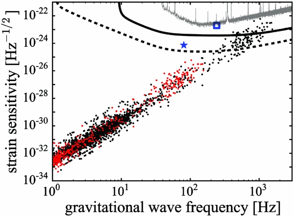
Figure 5. Peak gravitational wave amplitudes from superfluid turbulence from galactic pulsars with Ro = ΔΩ/Ω = 10−1 (black points) and 10−2 (red points). The blue star and square are hypothetical, nearby (d = 10pc) rapid rotators with spin periods p = 3 ms and 10 ms, and Ro = 10−2 and 10−1, respectively.
6.2. Stochastic background
A cosmological population of neutron stars with turbulent cores produces a stochastic gravitational wave background that peaks in aLIGOs most sensitive frequency band (Lasky, Bennett, & Melatos Reference Lasky, Bennett and Melatos2013). Although there are large uncertainties in the expected amplitude of the background due to a lack of understanding of ΔΩ, the shape of the spectrum is relatively unique, with it being well-approximated by a piecewise power-law Ωgw(f gw) = Ωαf αgw, with α = 7 and α = −1 for f gw < fc and f gw > fc, respectively. Here, fc is the population-weighted average of 1/τc, and Ωgw(f gw) is the energy density in the gravitational wave background as a fraction of the closure energy density of the Universe.
It is worth noting that turbulent convection in main-sequence stars also produces a gravitational wave signal (Bennett & Melatos Reference Bennett and Melatos2014). Interestingly, the loudest gravitational wave signal detectable on Earth may come from the Sun as, for frequencies f gw ≲ 3 × 10⁻⁴Hz, the Earth lies in the Sun’s near zone, in which the wave strain scales significantly more steeply with distance, h rms∝d −5 (cf. ∝d −1 in the far zone; Cutler & Lindblom Reference Cutler and Lindblom1996; Polnarev, Roxburgh, & Baskaran Reference Polnarev, Roxburgh and Baskaran2009). This gravitational wave signal is most relevant in the micro to nHz regime, and therefore most applicable to pulsar timing experiments. However, the gravitational-wave scaling at low-frequencies is uncertain as Kolmogorov scaling for turbulence breaks down below f gw ≲ 10−8Hz.
7 CONCLUSIONS
Ground-based gravitational wave interferometers are already contributing to our understanding of interesting astrophysical phenomena. But non-detections will only progress the field so far; the first direct detection of gravitational radiation will herald a new scientific field of study, and will allow new insight into the most exotic regions of our Universe.
While the first detection with aLIGO is expected to be from the inspiral and merger of a compact binary system, there are many unknown, and ill-understood, mechanisms that can generate gravitational waves with significant amplitudes from isolated neutron stars. This review highlights many of those mechanisms where we have some understanding of the key, physical processes. It also highlights the vast uncertainty of many of these predictions, showing that they rely on knowledge of neutron star physics beyond current capabilities. But this is what makes the field so fascinating; a positive detection of gravitational waves from any of the mechanisms discussed in this paper will allow an unprecedented view into the heart of neutron stars, where some of the most exotic physics in the Universe takes place.
ACKNOWLEDGEMENTS
PDL is supported by the Australian Research Council Discovery Project DP140102578. I am extremely grateful to Bryn Haskell, Daniel Price, Kostas Glampedakis, and Karl Wette for useful comments on the manuscript.


 Open access