2.1.1. Rebargaining

To introduce formally the notion that the contract may be rebargained in period 2 we let S_g (D_g (a ₁), ε _g ) be the utility of the household member of gender g if the marriage breaks up in that period. D_g (a ₁) is a division of family wealth in the event of divorce with the property ∑ _g D_g (a ₁) ⩽ a ₁. The following participation constraints have to be satisfied in t = 2.Footnote ⁴

\begin{equation*} V_g(a_1, \lambda _2, \epsilon ) \equiv u(c_2^g,l_2^g)+ \xi \ge S_g (D_g(a_1), \epsilon _g) \;\;\;\; \text{for} \;\;\;\; g \in \lbrace m, f \rbrace , \end{equation*}

where V_g is the level of utility that individual g derives when program (1) is solved.

Now, consider the previous example where $\lambda _1 = \frac{1}{2}$ and ε _m > >ε _f and assume that $V_m(a_1, \frac{1}{2}, \epsilon ) < S_m (D_m(a_1), \epsilon _m)$ , in other words that the male spouse’s participation constraint is violated. Assume further that there is a range of values [λ ^L ₂, λ₂ ^U ] with $\lambda _2^L>\frac{1}{2}$ so that (i) V_m (a ₁, λ ^L ₂, ε) = S_m (D_m (a ₁), ε _m ) and V_f (a ₁, λ ^L ₂, ε) > S_f (D_f (a ₁), ε _f ) and (ii) V_f (a ₁, λ ^U ₂, ε) = S_f (D_f (a ₁), ε _f ) and V_m (a ₁, λ ^U ₂, ε) > S_m (D_m (a ₁), ε _m ). Moreover, assume that for any λ₂ ∈ (λ ^L ₂, λ ^U ₂) the participation constraints are slack.Footnote ⁵

We need to find a value of λ₂ within [λ ^L ₂, λ₂ ^U ] so that the both constraints are satisfied. We choose a value λ₂ so that

(3) \begin{eqnarray} &&\lambda _2 \in \text{arg} \min _{\lambda ^*} | \lambda ^* - \lambda _1 | \nonumber\\ && \text{such that} \;\; \;\; V_g(a_1, \lambda ^*, \epsilon ) \ge S_g (D_g(a_1) ,\epsilon _g) \;\;\; \;g \in \lbrace m,f\rbrace . \end{eqnarray}

Note that (3) says that when there is a change in λ₂ relative to λ₁, this change is the minimum required to satisfy with equality the constraint which is violated. In terms of the previous example, we choose to set λ₂ = λ ^L ₂.

2.1.2. A representation with recursive contracts

It has been customary in the literature (see for example Cooley et al. (Reference Cooley, Marimon and Quadrini2004) and Kehoe and Perri (Reference Kehoe and Perri2002), among others) to solve dynamic limited commitment models using a Lagrangian formulation, then to apply the results of Marcet and Marimon (Reference Marcet and Marimon1994) to obtain the recursive representation of the program. It is useful to briefly illustrate that the above derivations are consistent with this approach, in particular the Bellman equations in (1) and (2) can be derived from the saddle point problem described in Marcet and Marimon (Reference Marcet and Marimon1994).

The maximization problem can be stated as follows:

\begin{eqnarray*} \begin{array}{c} \max _{c_1^g,l_1^g,c_2^g,l_2^g} E_1 \sum _{t=1}^2 \beta ^{t-1} \sum _g \overline{\lambda }_g u(c_t^g,l_t^g) \\[6pt] \text{subject to:} \;\; u(c_2^g,l_2^g)+ \xi \ge S_g (D_g(a_1), \epsilon _g) \\[6pt] E_1 \sum _{t=1}^2 \beta ^{t-1} u(c_t^g,l_t^g) + \xi (1+\beta ) \ge S_g (D_g(a_0), 1) \\[6pt] \frac{\sum _g c_2^g }{1+r(1-\tau _K)} +\sum _g c_1^g = a_0 (1+r(1-\tau _K)) + \frac{\sum _g (1-l_2^g) w \epsilon _g }{1+r(1-\tau _K)} + \sum _g (1-l_1^g) w, \end{array} \end{eqnarray*}

where the last equation is the intertemporal budget constraint of the household and a ₁ = a ₀(1 + r(1 − τ _K )) + ∑ _g (1 − l^g ₁)w − ∑ _g c^g ₁ also has to be remembered to find the optimum. $\overline{\lambda }_g$ are constant weights satisfying $\frac{\overline{\lambda }_m}{\sum _g \overline{\lambda }_g }=\lambda _1$ from the previous definition of the sharing rule.Footnote ⁶ Moreover, notice that for completeness we have now included in the constraint set the two participation constraints in period 1, i.e. E ₁∑² _{t = 1}β ^{t − 1} u(c^g _t , l_t ^g ) + ξ(1 + β) ⩾ S_g (D_g (a ₀), 1), where S_g (D_g (a ₀), 1) is the outside option in the first period. It is trivial to show that these constraints will not bind if for instance we set $\overline{\lambda }_m=\overline{\lambda }_f$ (because of ξ > 0).

Define x _{t, g} = 1 for t = 1 and x _{t, g} = ε _g , t = 2. The above program can be represented with the Lagrangian:

\begin{eqnarray*} L &=&E_1 \Bigg(\sum _{t=1}^2 \beta ^{t-1} \sum _g \Bigg (\overline{\lambda }_g u(c_t^g,l_t^g) + v_{t,g} \Bigg [\sum _{j=t}^2 \beta ^{j-1} (u(c_j^g,l_j^g)+ \xi )\nonumber\\ &&\qquad -\, S_g (D_g(a_{t-1}), x_{t,g})\Bigg ] \Bigg )\Bigg ) \\ &&+\, \phi \Bigg[ \frac{\sum _g c_2^g }{1+r(1-\tau _K)} +\sum _g c_1^g - a_0 (1+r(1-\tau _K))\nonumber\\ &&\qquad -\, \frac{\sum _g (1-l_2^g) w \epsilon _g }{1+r(1-\tau _K)} - \sum _g (1-l_1^g) w \Bigg], \end{eqnarray*}

where v _{t, g} is the multiplier on the participation constraint of g at t. Rearranging this expression, we can write:

\begin{eqnarray*} L &=&E_1 \Bigg (\sum _{t=1}^2 \beta ^{t-1} \sum _g \Bigg ( ( \overline{\lambda }_g +\overline{v}_{t-1,g} +v_{t,g} ) u(c_t^g,l_t^g) + (\overline{v}_{t-1,g} +v_{t,g} ) \xi\nonumber\\ &&\qquad -\, v_{t,g} S_g (D_g(a_{t-1}), x_{t,g})\Bigg )\Bigg )\\ && +\,\phi \Bigg[ \frac{\sum _g c_2^g }{1+r(1-\tau _K)} +\sum _g c_1^g - a_0 (1+r(1-\tau _K))\nonumber\\ && \qquad-\, \frac{\sum _g (1-l_2^g) w \epsilon _g }{1+r(1-\tau _K)} - \sum _g (1-l_1^g) w \Bigg], \end{eqnarray*}

where $\overline{v}_{t,g}=\overline{v}_{t-1,g} +v_{t,g}$ with $\overline{v}_{0,g}=0$ .

Marcet and Marimon (Reference Marcet and Marimon1994) show that the above program defines a saddle point problem which can be resolved through finding a minimum with respect to v _{t, g} (subject to v _{t, g} ⩾ 0) and a maximum with respect to consumption and hours. This problem can also be represented recursively with the Bellman equation. For the sake of brevity, we omit this derivation.

Note that the first order conditions with respect to c^g _t give: $\frac{u_c(c_t^m,l_t^m)}{u_c(c_t^f,l_t^f)} = \frac{\overline{\lambda }_f+\overline{v}_{t,f}}{\overline{\lambda }_m+\overline{v}_{t,m}}$ . It is well known that in the presence of limited commitment the ratio of marginal utilities is not constant over time, it varies when the participation constraints bind. Now consider the problem at hand: Obviously we can set $\overline{v}_{0,g}=0$ (as the initial condition) and also $\overline{v}_{1,g} =0$ (since the period 1 constraints can be ignored). In period 2, we can have any of the following (i) v _{2, m} > 0, v _{2, f} = 0 (male constraint binds), (ii) v _{2, m} = 0, v _{2, f} > 0 (female constraint binds) or (iii) v _{2, m} = 0, v _{2, f} = 0 (both constraints are slack). This means that the $\frac{u_c(c_t^m,l_t^m)}{u_c(c_t^f,l_t^f)}$ will either drop to $\frac{\overline{\lambda }_f}{\overline{\lambda }_m+\overline{v}_{t,m}}$ , increase to $\frac{\overline{\lambda }_f+\overline{v}_{t,f}}{\overline{\lambda }_m}$ or remain constant $\frac{\overline{\lambda }_f}{\overline{\lambda }_m}$ . Moreover, based on the above it is obvious that the adjustments in the weight in cases (i) and (ii) are the minimum required so that a participation constraint just binds.Footnote ⁷ In other words, the optimal contract described in the previous subsection is essentially what we get if we apply the method of Marcet and Marimon (Reference Marcet and Marimon1994).Footnote ⁸

2.2.1. Separable preferences

Let us first assume that γ equals one. Assume that we are in period 2 and let A_c = (1 + r(1 − τ _K ))a ₁ be the total financial income of the household brought forward from period one. It is trivial to show that the optimal consumption is c^m ₂ = λ₂η(A_c + ∑ _g w(1 − τ _N )ε _g ) and c^f ₂ = (1 − λ₂)η(A_c + ∑ _g w(1 − τ _N )ε _g ). Similarly, the optimal choice of leisure is given by: $l ^m_2= \lambda _2 (1-\eta ) \frac{ A_c + \sum _g w (1-\tau _N) \epsilon _g}{\epsilon _m w (1-\tau _N)}$ and $l ^f_2= (1- \lambda _2) (1-\eta ) \frac{ A_c + \sum _g w (1-\tau _N) \epsilon _g}{\epsilon _f w (1-\tau _N)}$ .

To respect the participation constraint of each household member the allocation rule λ₂ must satisfy the following conditions:

\begin{eqnarray*} &&\log \lambda _2^g + \eta \log \eta (A_c + w (1-\tau _N) (\epsilon _m+\epsilon _f))\nonumber\\ &&\quad +\, (1-\eta ) \log \eta \frac{(A_c + w (1-\tau _N) (\epsilon _m+\epsilon _f))}{\epsilon _g w (1-\tau _N)} \nonumber\\ &&\quad +\, \xi \ge\eta \log \eta \Bigg(\frac{A_c}{2} + w (1-\tau _N) \epsilon _g\Bigg) + (1-\eta ) \log \eta \frac{( \frac{A_c}{2} + w (1-\tau _N) \epsilon _g)}{\epsilon _g w (1-\tau _N)} ,\nonumber\\ &&\quad g \in \lbrace m,f \rbrace , \end{eqnarray*}

where the capital tax τ _K enters through A_c . Solving these conditions for λ₂ we get

(4) \begin{eqnarray} \lambda _2 \in \left\lbrace \underbrace{ e^{-\xi } \frac{ \frac{A_c}{2}+\epsilon _m w (1-\tau _N)}{A_c + \sum _g \epsilon _g w (1-\tau _N)}}_{ \lambda _2^L}, \;\; \underbrace{ 1-e^{-\xi } \frac{ \frac{A_c}{2}+\epsilon _f w (1-\tau _N)}{A_c + \sum _g \epsilon _g w (1-\tau _N)} }_{ \lambda _2^U} \right\rbrace . \end{eqnarray}

Expression (4) defines the upper and the lower bound we have previously seen. Given ε _f and A_c , there is a threshold $\underline{\epsilon }_m(A_c, \epsilon _f )$ such that if $\epsilon _m > \overline{\epsilon }_m(A_c, \epsilon _f)$ the contract updates λ₂ to be equal to the lower bound in (4) (since in that case it holds that $\lambda _2^L> \frac{1}{2}$ ). Similarly, there is another threshold $\underline{\epsilon }_m (A_c, \epsilon _f)$ such that for an ε _m below this threshold the new contract gives λ₂ equal to $\lambda _2^U < \frac{1}{2}$ . Notice that when ξ = 0, λ ^L ₂ equals λ ^U ₂. In this case, the intrahousehold allocation is such that in every state a household member’s share on total resources is essentially what they would get as a single. Being together is therefore no different than being single when ξ = 0.Footnote ⁹

Labor Taxes. Given the intrahousehold allocation, we can derive the effect of changes in the level of labor taxes τ _N and capital taxes τ _K . First, consider that labor taxes fall, i.e. (1 − τ _N ) increases. We can write

(5) \begin{equation} \frac{d \lambda _2^L}{\ d \; (1-\tau _N) } = e^{-\xi } A_c \frac{ \epsilon _m w- \frac{\sum _g \epsilon _g w}{2} }{ (A_c +\sum _g \epsilon _g (1-\tau _N) w) ^2}, \end{equation}

Consider the case where $\epsilon _m > \overline{\epsilon }_m (A_c, \epsilon _f)$ . It must be that $\lambda _2 = \lambda _2^L>\frac{1}{2}$ , i.e. the male spouse’s weight needs to increase. The derivative (5) is positive, meaning that a reduction in the level of labor taxes increases λ ^L ₂, this makes the change in λ₂ relative to λ₁ even greater. Therefore, a drop in the tax rate reduces risk sharing within the household; in those states where the male labor income is high, the husband’s consumption share increases even more than if labor taxation is high.

A similar argument can be made for the case where ε _f ≫ ε _m , i.e. when the upper bound λ ^U ₂ is relevant. We summarize the result in the following proposition:

Proposition 1. Assume that the household’s financial income is positive ( A_c > 0). A reduction in labor income taxes reduces insurance within the household under log-separable preferences. The household sharing rule and thus the intrahousehold allocation become more responsive to changes in idiosyncratic productivity. Footnote ¹⁰

The intuition for this result is as follows: First, note that inequality in labor income is the root of the limited commitment problem in the model. Therefore, a policy reform which lowers the tax rate, exacerbates the intrahousehold income inequality and exacerbates the limited commitment problem. This effect is captured by the fact that the partial derivative $\frac{d \lambda _2^L}{\ d \; (1-\tau _N) }$ is positive, at least insofar as financial income is positive. Second, to understand why wealth is important notice that the labor taxes, besides making the distribution of the net labor income more equitable in the household, they also impoverish the household by reducing its disposable income. When the household has fewer resources the temptation to renege on the marital contract is stronger, this makes the limited commitment problem more severe. This effect under log-separable utility is relevant only insofar as A_c < 0. However, for the case where γ > 1 the effect will be present even if the household has savings rather than debt. We will return to this feature of the model in a subsequent paragraph.

Capital Taxes. We now derive the impact of wealth and capital taxation on the participation constraints. For brevity, consider the partial derivative of λ ^L ₂ with respect to 1 − τ _K :

(6) \begin{eqnarray} \frac{d \lambda _2^L}{\ d \;(1- \tau _K)} = e^{-\xi } (1-\tau _N) \frac{ \frac{\sum _g \epsilon _g w}{2} - \epsilon _m w }{ (A_c +\sum _g \epsilon _g (1-\tau _N) w) ^2} a_1 r, \end{eqnarray}

Notice that if ε _m > ε _f (male participation constraint may bind and λ ^L ₂ is relevant), then (6) gives $\frac{d \lambda _2^L}{\ d \; (1- \tau _K)} <0$ . This implies that a rise in asset income increases intrahousehold household risk sharing.

Proposition 2. Lower capital taxes improve insurance under log-log preferences. The household sharing rule and thus intrahousehold allocation are less responsive to changes in labor income.

Several remarks are in order: First, equations (5) and (6) reveal that the effects of taxes depend on the wealth level of the household. The higher wealth is, the bigger the impact of the tax schedule on the intrahousehold allocation. This implies that richer households are more likely to benefit from a change in policy which eliminates capital taxes. However, for these households the limited commitment friction is less severe, precisely because wealth is high. This property is key to understanding the modest effects from the reform that we uncover in our quantitative exercise in the next sections.

Second, it is important to emphasize that the improvement in intrahousehold insurance identified in Proposition 2 does not stem from the standard role of assets as a buffer against income shocks (e.g. precautionary savings) but is related to the division of resources in the household and the notion that wealth, in contrast to labor income, is a common resource for the household. This channel is new to the literature.

2.2.2. Non-separable preferences

We now derive the impact of changes in taxation assuming γ > 1. We can write the participation constraints as follows:

\begin{eqnarray*} &&\left( s_g (\lambda _2, \epsilon )\frac{A_c + w (1-\tau _N) (\epsilon _m+\epsilon _f) }{((w (1-\tau _N) \epsilon _g) )^{1-\eta }} \right)^{1-\gamma } \frac{\chi }{1-\gamma }\nonumber\\ &&\quad +\, \xi \ge \left(\frac{\frac{ A_c}{2} +w (1-\tau _N) \epsilon _g }{(w (1-\tau _N) \epsilon _g)^{1-\eta }} \right)^{1-\gamma } \frac{\chi }{1-\gamma }, \end{eqnarray*}

where χ = (η^η(1 − η)^{1 − η})^{1 − γ} and $s_m(\lambda _2 ,\epsilon ) = (\frac{\lambda _2}{1-\lambda _2} ( \frac{\epsilon _f}{\epsilon _m})^{(1-\eta ) (1-\gamma )} )^{1/\gamma }-1$ , s_f (λ₂, ε) = 1 − s_m (λ₂, ε). We show in the Appendix that the sign of the effect of a rise in 1 − τ _N on λ ^L ₂ is inversely related to the sign of the following expression:

(7) \begin{eqnarray} &&(1-\gamma )\left[ \tilde{\xi } \left(\frac{A_c (1-\eta )}{1-\tau _N}-\eta \sum _g w \epsilon _g \right) \kappa _1 (A_c ,\epsilon )\right.\nonumber\\ &&\quad\left. +\, \left( A_c w \left( \epsilon _m - \frac{\sum _g \epsilon _g}{2}\right)\right) \kappa _2(A_c , \epsilon ) \right], \end{eqnarray}

where $\kappa _1 = \frac{ (w (1-\tau _N) \epsilon _m)^{(1-\eta )(1-\gamma )}}{(A_c + \sum _g w (1-\tau _N) \epsilon _g )^{2-\gamma }} >0$ , $\kappa _2 = \frac{(\frac{A_c}{2} +w (1-\tau _w) \epsilon _m )^{-\gamma } }{( A_c + \sum _g w (1-\tau _w) \epsilon _g )^{2-\gamma } } >0$ and $\tilde{\xi } = \frac{ -\xi (1-\gamma )}{ \eta ^{\eta } (1-\eta )^{1-\eta }} >0$ .

In (7), if A_c = 0, only the leading term is different from zero and in fact it is positive. In this case, we can show that an increase in 1 − τ _N will increase intrahousehold risk sharing or, to put it differently, it will reduce the response of the sharing rule to variations in income. When A_c > 0, the second term is added and also the first term in (7) eventually switches sign. When the overall partial derivative is negative, the fall in labor taxation exacerbates inequality within the family and reduces risk sharing. This is the result we established under log-separable utility. What non-separability brings to the equation is the leading term in (7) which yields the non-monotonicity that makes the effect of changes in labor income taxation ambiguous.

To understand what this term captures, note that as discussed previously, a rise in the tax rate reduces inequality in terms of labor incomes but it also impoverishes the household. When utility is curved, the reduction in household income translates into an increase in the marginal utility which tightens the participation constraints. In the case of log utility, this effect was balanced by the larger equity in household resources; it dominated only when the household had negative savings. But under γ > 1 the income effect may dominate even when household financial income is positive.

In the Appendix, we show that a similar result applies to the upper bound λ ^U ₂. We also establish that the effect of lower capital taxation is unambiguous; it always improves the household’s insurance possibilities.

Proposition 3. Assume A_c > 0 and γ > 1. Lowering labor income taxes reduces intrahousehold risk sharing when household wealth is low. In contrast, when the household is wealthy, reducing labor taxation has a detrimental effect on intrahousehold insurance. Lower capital taxes always improve the household’s insurance possibilities.

Proof: See Appendix.

In our quantitative analysis in Section 5, following the rest of the macro literature on optimal taxation, we focus on the case of non-separable utility. It is however important to disentangle the channels through which preferences affect our results, and for this purpose we also considered separable preferences. Note that since the change in policy considered in Section 5 is one which eliminates capital taxation and raises labor income taxes, our results under non-separable utility illustrate that for some households, the limited commitment problem may even be more severe after the reform. This could be the case for young households which are typically wealth poor.

3.4.1. Bachelor households

We first consider the program of a bachelor of gender g and age j. We let S_g (a, X, j) be the lifetime utility for this agent when her (his) stock of wealth is a, her permanent productivity is α _g , her idiosyncratic time varying productivity is ε _g . To save on notation, we summarize the fixed effect and the time varying component of productivity in a vector X. The agent must choose consumption c and hours worked n (if not retired, i.e. j < j_R ) to maximize her utility subject to the budget and the borrowing constraints. She solves the following functional equation:

(9) \begin{eqnarray} S_g (a, X , j ) &=& \max _{c,l,a^{\prime } \ge 0 , l} u(c,l) + \beta \psi _j \int S_g(a^{\prime },X^{\prime } , j+1 ) d \pi _g (X^{\prime }| X),\\ &&\text{Subject to:} \;\;\;\; l+n \le 1 \nonumber \\ a^{\prime } + (1+\tau _C) c &=& (a+B) (1+r(1-\tau _K))\nonumber\\ && +\, w \epsilon _g \alpha _{g} L_g(j)(1-\tau _N -\tau _{SS}) n \; \text{ if } j <j_R \nonumber \\ a^{\prime } + (1+\tau _C) c &=& (a+B) (1+r(1-\tau _K)) + SS( g, \alpha _{g}) \; \text{ if } j \ge j_R. \nonumber \end{eqnarray}

3.4.2. Couples

In this paragraph, we describe the program of the couple. Because the optimization problem was previously discussed, here we simply show the Bellman equations in the life cycle model of this section. Let λ and 1 − λ be the shares of the male and the female spouses respectively and M(a, X, λ, j) be the value function of a household of age j, where X summarizes the productive endowments of its members.Footnote ¹³ As before a is the level of wealth, and ξ is the (constant) benefit that accrues to each spouse in the marriage. The program of the couple can be written as:

\begin{eqnarray*} M(a,X,\lambda ,j ) &=& \max _{c^g,l^g,a^{\prime }\ge 0} \lambda u(c^m,l^m) + (1- \lambda ) u(c^f,l^f))\nonumber\\ && +\, \xi + \beta \psi _j \int M(a^{\prime }, X^{\prime } , \lambda ^{\prime }, j+1 ) d \pi (X^{\prime } | X), \nonumber \\ &&\text{Subject to:} \;\;\;\; l^g+n^g \le 1 \;\;\; \text{ for }\;\; g \in \lbrace m, f\rbrace \nonumber \\ a^{\prime } + (1+\tau _C)(c^m +c^f) &=& (a+2 B) (1+r(1-\tau _K))\nonumber\\ && +\, w \Big ( \sum _g L_g(j) \alpha _i \epsilon _{i,g} n^g (1-\tau _N -\tau _{SS} )\Big ) \; \text{ if } j <j_R\nonumber \\ a^{\prime } + (1+\tau _C)(c^m +c^f) &=& (a+2 B) (1+r(1-\tau _K)) + \sum _g SS( g, \alpha _{g}) \; \text{ if } j \ge j_R,\nonumber \end{eqnarray*}

where the updating of the sharing rule for λ (which generalizes the analogous object in Section 2) is

(10) \begin{eqnarray} &&\lambda ^{\prime } \in \text{arg} \min _{\lambda ^*} | \lambda ^* - \lambda | \;\;\; \text{such that} \\ &&V_g(a^{\prime },X^{\prime } ,\lambda ^*,j+1 ) \ge S_g \left(\frac{a^{\prime }}{2} , X_g^{\prime } , j+1 \right). \nonumber \end{eqnarray}

X_g is a vector formed by elements of X that are relevant to household member g if he or she were to be single. V_g is the lifetime utility that individual g derives when program (3.4.2) is solved.

We assume that value of λ is initiated at the matching stage of the life cycle as a solution to the following Nash bargaining problem:

(11) \begin{eqnarray} &&\lambda _1 \in \text{arg} \max _{\lambda } \left[ V_m(a,X ,\lambda ,1 ) - S_m\left( \frac{a}{2},X ,\lambda ,1 \right) + \overline{\xi }_m \right] \; \Big[ V_f(a,X ,\lambda ,1 )\nonumber\\ &&\quad - S_f\left(\frac{a}{2},X ,\lambda ,1 \right) + \overline{\xi }_f \Big]. \end{eqnarray}

Notice that the Nash sharing rule determines the initial allocation under the influence of two gender specific utility gains $\overline{\xi }_g$ for g ∈ {m, f}. Since we will assume that $\sum _g \overline{\xi }_g =0$ , $\overline{\xi }_m$ and $\overline{\xi }_f$ do not affect the marital surplus, they simply determine the share of the surplus which each spouse receives.Footnote ¹⁴

We will use these terms to determine the magnitude of income transfers from one spouse to the other; the ultimate goal is to make the model match the inequality in hours between married men and women that we observe in the data. If $\overline{\xi }_m >0$ and $\overline{\xi }_f<0$ then the household contract will give an initial allocation with large transfers from the male to the female spouse, this will lead to substantial inequality in hours within the family. Because the updating rule (10) will make λ persistent over time (we will demonstrate this in a later subsection) inequality in hours will carry over in subsequent periods.

Note that an alternative way to target the hours inequality would be to simply pick the initial shares (as we did in Section 3 for instance). However, we need to close the model with the Nash rule in (11) for the following reason: When we consider the change in the tax policy, the intrahousehold allocation may be impacted through changes in the initial value of λ. These changes would be absent if we fixed exogenously the initial share, and they may have significant effects on the welfare gains of husbands and wives.

We characterize the competitive equilibrium in Section A.2 in the Appendix.

4.1.1. Preferences and demographics

The demographic parameters have been set so that the model has a stationary demographic structure that matches the age distribution in the US economy. We assume that individuals are born at age 25 and live at most until age 95. Retirement is at age 65. The survival probabilities are taken from Arias (Reference Arias2010), based on the US National Vital Statistics Reports and correspond to probabilities concerning the entire population (pooling men and women). The model period is set to five years. This means that there are fifteen periods and the retirement age is j_R = 10. Although we make this assumption for computational reasons, in what follows we report annual values for the parameters.

We set the fraction of households that are married (μ) equal to 52%, which is the corresponding statistic in the PSID data over all age groups. Population growth is assumed to be θ = 0.012. We calibrate the preference parameters as follows: first, we follow Conesa et al. (Reference Chiappori2009) and Fuster et al. (Reference Fuster, Imrohoroglu and Imrohoroglu2008), and set γ = 4.Footnote ¹⁵ We also choose a value of η = 0.41 so that our model gives in the steady state average hours worked of one third. With these numbers the intertemporal elasticity of substitution, (1 − η(1 − γ))^{− 1}, is equal to 0.4484.

For married couples we have to determine the utility gains $\overline{\xi }_m$ and $\overline{\xi }_f$ at the Nash bargaining stage, and the flow gain ξ that couples enjoy at each period. As discussed earlier, these parameters govern the following two aspects of the intrahousehold allocation: First, $\overline{\xi }_m$ and $\overline{\xi }_f$ determine the transfers from one spouse to the other, and along with differences in the age productivity profiles L_j (g), they determine inequality in hours within the household. We pick numbers for these parameters to match average hours worked for married men and women as in the US data; according to the PSID married males worked 2104 hours in 2006, married females 1420 hours.Footnote ¹⁶ We map these numbers into model units.Footnote ¹⁷ $^,$ Footnote ¹⁸

Second, ξ determines the ability of the household to commit to a sharing rule λ. The smaller ξ is, the more the household members will be tempted to renege on this rule and the more frequent rebargaining will be. Our strategy to calibrate the value of ξ is the following: We choose a value that is as low as possible so that we maximize the frequency of rebargaining in the model but also so that divorce never occurs in equilibrium. We find that a value ξ = 1.2 is appropriate to accomplish this goal. To show what this means we have calculated the compensating variation, the increment in consumption that the average married individual would require to be as well-off as if we set ξ = 0. We obtained a value equal to 19.8% of average consumption. Therefore, the model predicts a substantial utility gain from being married.Footnote ¹⁹

There are two model mechanisms which explain this finding: First, because of the fixed effects which maybe high for one spouse and low for the other, we need a large gain to keep the couple together. Since the α _g are permanent characteristics, there is virtually no insurance value accruing to a couple for which α _m ≫ α _f , this basically says that we cannot sustain any mutual insurance arrangement against this shock.Footnote ²⁰

The second reason is the presence of wealth in the model. We previously saw in the two period model that a couple would remain married even if we set ξ = 0 in t = 2 (in that case the intrahousehold allocation gives to each individual what they would get as a single). This also holds in the multiperiod setup if families cannot save (or if they can save in separate accounts). But with common wealth in the household it does not hold. To understand why suppose that the husband draws a high value of ε _m today. If the couple divorces, then high productivity leads to more savings for the husband and persistently higher consumption. If they do not divorce, then wealth needs to be shared and (partly) used to finance a higher consumption level for the wife. Unless we assume ξ > 0, the marital surplus becomes negative and the couple divorces. We will comment further on this feature of the model in a subsequent section.

4.1.2. Technology and endowments

The technology parameters are chosen as follows: We allow A_t to grow at a rate equal to 1.4% per year.Footnote ²¹ Moreover, following Fuster et al. (Reference Fuster, Imrohoroglu and Imrohoroglu2008) we set the capital share in value added ζ equal to 0.36 and we choose the depreciation rate of capital δ to match an investment to output ratio of 21% in the steady state. This gives us an annual value for this parameter of 5.26%. The subjective discount factor β is calibrated so that the economy in the steady state produces the capital output ratio of 2.7. This procedure yields a value of 0.998.

Individual wages in the model are the product of three components; the gender specific life cycle profile, the fixed effect, and the temporary idiosyncratic productivity shock, i.e. L_g (j)α _g ε _g . Following the bulk of the literature we take the life cycle profiles L_g (j) from Hansen (Reference Hansen1993). Moreover, our principle to calibrate the fixed effect component and the distribution of the idiosyncratic shocks ε is to reproduce the life cycle pattern of the cross-sectional variance of the log of family earnings as is documented in Storesletten et al. (Reference Storesletten, Telmer and Yaron2004).

As in Storesletten et al. (Reference Storesletten, Telmer and Yaron2004) we assume that both α _g and ε _g are log-normally distributed random variables. The fact that these variables in the model are represented as discrete may be thought as an approximation of the processes using standard techniques (for example Adda and Cooper (Reference Adda and Cooper2003)). For the fixed effect, we have chosen two values (α₁, α₂), these are common across gender and marital status. We follow Conesa and Krueger (Reference Conesa and Krueger2006) and set α₁ = e ^{− σ_α} and α₂ = e ^σ_α (where σ_α governs the variance of the process) and (for bachelor) agents we calibrate $p^S_{g}(\alpha _1)=p^S_{g}(\alpha _2) =\frac{1}{2}$ . This is an obvious choice since if we apply any standard numerical discretization procedure to approximate a continuous log normal variable with a constant variance we will get probabilities equal to 1/2.

For couples, we calibrate the joint probabilities p^M (α _m , α _f ) so that our economy reproduces the degree of marital sorting in earnings ability that has been documented in the US data; for instance Hyslop (Reference Hyslop2001) estimates a 0.5 correlation of fixed effects within the family in his PSID sample. We will choose the pdf p^M (α _m , α _f ) to match this correlation coefficient. To explain how this is done, note that for married individuals the process α _g again takes two values α _g ∈ {e ^{− σ_α} , e ^σ_α }. This gives us the following combinations for the pair: (α _m , α _f ) ∈ {(e ^{− σ_α} , e ^{− σ_α} ), (e ^{− σ_α} , e ^σ_α ), (e ^σ_α , e ^{− σ_α} ), (e ^σ_α , e ^σ_α )}. p^M (α _m , α _f ) then gives the probability of having any one of these pairs. To match a correlation coefficient of 0.5 we have to set p^M ((e ^{− σ_α} , e ^{− σ_α} )) = p^M ((e ^σ_α , e ^σ_α )) = 0.375 (i.e. for spouses who have the same fixed effect). For the remaining nodes we set the probabilities equal to 0.125.

Analogously the stochastic process of the logarithm of ε has the following AR(1) representation:

\begin{equation*} \text{log}( \epsilon _{t}) = A \text{log} ( \epsilon _{t-1}) + u_{t}, \end{equation*}

where u _{(2 × 1)} is a vector of shocks to productivity and follows $\mathcal {N} (0_{(2\times 1)}, \Sigma _u)$ and Σ _u is the variance covariance matrix of the shocks. The diagonal elements of Σ _u are σ² _u , the off-diagonal elements (covariances) are $\sigma _{u_1,u_2}=\tilde{\rho }_{u_1,u_2} \sigma _u^2$ where $\tilde{\rho }_{u_1,u_2}$ is the correlation coefficient of the two shocks. We set $\tilde{\rho }_{u_1,u_2} =0.15$ following the empirical evidence presented in Hyslop (Reference Hyslop2001). Finally, let $A =\rho _{\epsilon } \mathcal {I}_{2\times 2}$ where $\mathcal {I}_{2\times 2}$ is the identity matrix and ρ_ε is the first order autocorrelation coefficient of the ε process.

The above stochic process is also applied to bachelor households, so the parameters ρ_ε and σ _u are common to singles and couples.

We now have three numbers to pick: ρ_ε, σ_α and σ _u . We proceed as follows: First, we choose σ_α to reproduce the cross-sectional variance of the logarithm of household labor income (pooling bachelors and couples) at age 25 reported in Storesletten et al. (Reference Storesletten, Telmer and Yaron2004). This target gives us σ_α = 0.2. Second, we choose ρ_ε and σ _u so that we can get a cross-sectional variance which rises linearly with age and reaches 0.9 at age 65. This procedure gives ρ_ε = 0.89 (a yearly analogue of 0.977) and σ _u = 0.05 (yearly analogue of 0.0108). The stochastic process is then discretized using nine nodes. To obtain an approximation which gives a positive correlation between the u shocks, we apply the methodology of Burnside (Reference Burnside, Marimon and Scott1999).

4.1.3. Government

In order to parameterize the steady state tax code we proceed as follows: The level of expenditures G is chosen so that on the balanced growth path the government consumes 21% of output. This spending is financed by the tax levies on consumption, capital and labor income. We follow Fuster et al. (Reference Fuster, Imrohoroglu and Imrohoroglu2008) and fix the consumption tax τ _C to 0.05 and the capital income tax τ _K to 0.35. The value of τ _N is then chosen so that the government runs a balanced budget. In the initial steady state, the model gives us a value of roughly 15% for this parameter. In our numerical experiment, we eliminate capital income taxation and adjust labor income taxes while holding the level of expenditures constant to their steady state value.

Our principle to calibrate the social security benefit system is the following: First, as explained previously, we consider the individual as the unit to which benefits are distributed and not the household. Second, we try to capture in a parsimonious way, with the functional SS(g, α _g ), the fact that social security in the US contains a redistributive component. For instance, in 2004 individuals received 90% of the first $7,300 of their total social security entitlement, 32% for earnings between $7,300 and $44,000, and 15% for earnings above $44,000.Footnote ²² We calibrate SS(g, α _g ) so that the model economy gives roughly the same redistribution of income in retirement in terms of median lifetime earnings as in the US economy. To give an idea of the numbers, we calculate that men of the highest earning ability (fixed effect) get roughly 1.3 times as much as men of the lowest ability, whereas their lifetime earnings are twice as high. Furthermore, women with the lowest ability receive in benefits roughly 67% of what poor men receive, and women of high ability get slightly (3%) more than poor men. We fix the social security tax rate at 12.5% and solve for the average level of benefits. In the computational experiment, we keep the tax rate constant across environments and vary the level of benefits. We summarize the calibrated parameters in Table 1.

Table 1. Calibrated parameters

For growth rates ( $\hat{A}$ , θ, δ) the reported values are annual, but we solve on 5-yearly frequency.

5.3.1. Sharing rule

Consider again Figure 1 where we showed the behavior of the sharing rule for a typical couple and over time. The bottom panel of the figure represents with the dashed line the path of λ, in the final steady state and with the crossed line the analogous path in the first period of the transition. The solid line represents the initial steady state (same as in the top left panel).

Notice first that after the reform, the couple at age 25, draws a starting value of the weight that is different from the value in the initial steady state. The reform, therefore, has a differential impact on the male and the female spouses and redistributes bargaining power within the household. We will return to this model feature in a subsequent paragraph.

Second, note that in the new steady state with zero capital taxation, the household can better commit to this initial allocation and changes in the share are smaller. This effect is consistent our previous findings. Indeed the rise in λ at age 40 is roughly 8 percentage points in the final steady state, where as it is roughly 12 percentage points before the reform.Footnote ²⁹

Are these changes large enough to impart a big effect on individual consumption and on the intrahousehold allocation? The answer is probably not. To see this note that under non-separable preferences the share of the female spouse on total household consumption is given by

(12) \begin{eqnarray} s_f = \left(\frac{\lambda _2}{1-\lambda _2}( \frac{w_f}{w_m})^{(1-\eta ) (1-\gamma )} \right)^{1/\gamma }, \end{eqnarray}

and w_g = wL_g (j)α _g ε _g .

According to (12), the female consumption share changes either due to changes in the ratio $\frac{w_f}{w_m}$ (which correspond to the efficient allocation) or due to changes in the sharing rule λ (which are ex ante inefficient). In the case where the female wage drops by a third in the original steady state, her share of consumption drops by 8.7 percentage points. Removing the volatility of the share λ (i.e. imposing λ = 0.5 throughout) reduces the drop to 4.6 percentage points. Under the new tax schedule (in the final steady state) the reduction is in the order of 7.9 percentage points.

We see that in the final steady state there is a benefit measured in reduced consumption variability, but overall it seems quite modest, at least relative to a full commitment allocation which keeps λ equal to 0.5. Notice however that since the effects are permanent it is possible that even a small (per period) change represents a considerable benefit for the individual. We will resolve this issue in a later paragraph.

5.3.2. Household rebargaining

In order to further investigate the impact of the reform on intrahousehold commitment let us return to the statistics reported in Table 3. As the results in Column 2 show, the change in policy causes a drop in the frequency of rebargaining by about 3.2 percentage points in the new steady state. Between ages 25 and 45 contracts are renegotiated nearly 10% less frequently, for households aged 50 to 65 roughly 39% less frequently, and for retired households roughly 78%. The largest drops (in percentage terms) are therefore experienced by older households. Our model produces similar results for the first period of the transition (e.g. Column 3 of the table).

These effects are clearly modest and it would be surprising if they contributed considerably towards increasing intrahousehold risk sharing for the following reasons: First, because as discussed previously, young households which bargain more frequently experience only a moderate drop in rebargaining (in fact there is a rise in rebargaining at age 25 as households start their working lives with zero wealth). Second, because older households rebargain too little anyway since they own sufficient wealth in the initial steady state and therefore do not benefit from the more substantial loosening of the limited commitment friction.

5.3.3. Partial equilibrium effects

The last two columns of Table 3 present statistics drawn from a partial equilibrium analysis. In the column labeled ‘Only τ _K ’ we consider setting the capital tax equal to zero, and keeping all other quantities (taxes, wages, interest rates, etc.) to the original steady state values. The column labeled ‘Only τ _N ’ refers to a model where the labor tax increases to the final steady state value and all other aggregates are kept constant.

Two remarks are important: First, as we noted in Section 2.2, increasing labor taxation may, or may not, lead to less frequently binding participation constraints when γ > 1. On the one hand, as after-tax income inequality within the household is reduced, rebargaining will probably occur less often; on the other, when total household labor income is lower, the temptation to renege on the contract increases. The results shown in Column 5 demonstrate that overall the second channel dominates. Therefore, it is only the reduction in τ _K in the model which improves commitment. Second, these results confirm that accounting for general equilibrium effects is important to not overstate the gains from the reform on the intrahousehold allocation. In Section 2.2 we had stated our analysis in partial equilibrium, but we had explained that movements in interest rates and wages may mitigate the effects of changes in the tax schedule. The results shown in the last columns of the table are in line with this intuition.

5.3.4. Consumption volatility effects of improved commitment

When shocks to individual labor income occur, individual consumption is affected more if the household sharing rule changes. In the case where λ is constant over time, intrahousehold risk sharing is maximized. This corresponds to a full commitment allocation. When λ is updated frequently in response to shocks, intrahousehold insurance is weakened. We measure the effects of the policy change on the volatility of individual consumption in Figure 3. We have computed the conditional standard deviation of the log of consumption for each individual from a panel of 3,60,000 individuals and averaged by age group. Subsequently, we have computed the percentage changes in the volatility in various models relative to the original steady state. The figure reports these changes.Footnote ³⁰

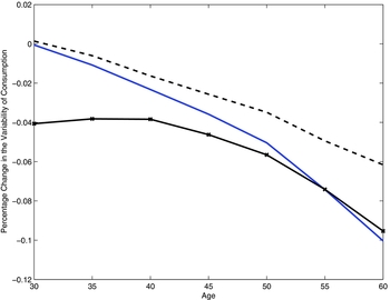
Figure 3. Individual Consumption Uncertainty.

Note: The figure plots changes in the variance of individual consumption relative to the original steady state. The solid line is the change in the final steady state. In order to measure the contribution of improved commitment, in the dashed line we represent the change in consumption volatility when we remove the influence of wealth but allow the household to be able to commit to the allocation as in the new steady state. For the sake of comparison, the crossed line in the figure represents a constant λ (full commitment) allocation.

The solid line represents the change in the final steady state. Notice that individual consumption uncertainty drops over the working life. By age 40, there is a 2% drop in the standard deviation and by age 50 a 4% drop. There are two possible explanations for this: First, more commitment, under the new policy, improves risk sharing (owing to the fact that families rebargain less frequently as we previously established). Second, higher wealth permits to the household to smooth the impact of shocks to consumption (e.g. through precautionary savings).

In order to measure the contribution of improved commitment in the dashed line we represent the change in consumption volatility when we remove the influence of wealth but allow the household to be able to commit to the initial allocation as in the new steady state. We accomplish this by keeping wealth constant as in the initial steady state and simulating household behavior under the final steady state paths for λ.

The graph indicates that across all age cohorts (with the exception of age 30), more commitment accounts for roughly 50% of the overall drop in consumption variability, the remaining 50% being accounted for by wealth.Footnote ³¹ Notice however that these changes are again not a significant improvement; they do not lead to a large drop in consumption uncertainty for young individuals, that typically face higher consumption variability. Therefore, the new policy confers only a small improvement in terms of reducing variability when variability is high and rather it reduces uncertainty when households have already build-up wealth so that the overall consumption uncertainty is smaller.

To further highlight these findings, in the crossed line in the figure we represent a constant λ (full commitment) allocation with household wealth as in the initial steady state. Under full commitment, there is a much larger reduction in consumption uncertainty at young ages. We conclude that at least for young households, the policy reform does not bring the allocation sufficiently close to the full commitment benchmark.

5.3.5. Conditional volatility of the sharing rule

In this paragraph we illustrate the effects of the change in taxes separately by household age and wealth. In Figure 4, we show the standard deviation of the share λ across different age groups and for different wealth levels. The solid line shows this standard deviation when households are at the borrowing constraint (age varies along the horizontal axis but initial wealth is kept constant for each age group). The dashed line represents the analogous object when initial wealth is set equal to the average wealth of families with the lowest fixed effect. The crossed line corresponds to the average wealth in the economy as the initial condition. The left panel in the figure represents the initial steady state and the right panel the final steady state. The figure shows clearly the influence of age and wealth on commitment that we previously identified.Footnote ³²

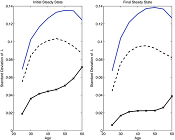
Figure 4. Volatility of the Sharing Rule.

Note: The figure plots the standard deviation of λ for various age groups, controlling for wealth. For each age, we have computed the share for all possible realizations of the state vector in the next period. In the solid line, we represent the standard deviation of the sharing rule when the household is at the borrowing constraint. In the dashed line wealth is at the average of the low fixed effect families in the model. In the crossed line wealth is set equal to the average wealth in the economy.

Let us now look at how these curves shift in the final steady state. Notice that the only curve which shifts downwards (thus showing a reduction in the variance of λ) is the crossed curve. Basically, households with very little initial wealth do not gain at all from the reform in terms of commitment. Wealthier households gain more, at the same time these households suffer much less from the limited commitment friction. This is another way of summarizing the modest impact from policy found in the previous paragraphs.

5.4.1. Division of welfare gains and loses within the household

Married men do better than married women according to the welfare measure in Table 6. This may seem surprising in light of the fact single women do better than single men. However, the outside options of married individuals exhibit a different welfare response to the reform because the wealth profiles between singles and couples are different.

To explain why married women do worse than married men note that as we have previously shown, after the reform couples are better able to commit to the initial allocation. This is a crucial observation because in our calibration we gave to women a large initial share (low λ) to match average hours as in the data. Consequently, in the model married men seek to rebargain after a few periods when male (relative to female) life cycle productivity grows. The expectation of this future rebargaining makes men willing to tolerate a lower starting value of λ in the initial steady state. When the tax code changes, however, and commitment to the initial allocation improves, married men anticipate a smaller renegotiation of the contract in the future. In effect, they want an increase in λ at the matching stage to compensate. Consistent with this view our model generates an increase in the average male share at the initial allocation by roughly one percentage point.

5.4.2. Welfare gains from commitment

Our theory predicts that lowering capital taxation affects intrahousehold risk sharing and lowers individual consumption uncertainty. In this paragraph, we investigate whether the improvement in insurance possibilities documented previously generates substantial welfare gains to households. In order to isolate the effect of ‘more commitment’ from changes in the wealth paths, we keep wealth constant as in the old steady state. We consider the following cases: 1. the household is able to commit as in the final steady state (the paths of λ are those of the final steady state), 2. the household can commit as in the old steady state (the paths of λ are those of the old steady state) and 3. the household can fully commit (λ is constant over time). To calculate the welfare benefit from commitment we compute the average value of the compensating variation between 2. and 1. In order to quantify how far this welfare gain is from the full commitment allocation we compare 2. and 3.

Our results are as follows: First we find that the welfare gain from improved commitment in the final steady state is tiny, roughly 0.062% of consumption. Second, we obtain a welfare gain from full commitment that is substantial, roughly 0.82% of consumption. These results reinforce our previous findings.

5.5.1. Log-separable utility

We briefly discuss the effects of the reform when utility is separable in consumption and leisure. In this version of our model, we keep all of the parameters as in the benchmark.Footnote ³⁸ We find that in the old steady state, families rebargain 10.47% on average. This fraction is 12.58% for ages 25–45, 11.30% between ages 50 and 65 and 0.26% in retirement. In the new steady state, overall rebargaining drops to 9.83%. For the age groups we obtain 13.06%, 8.48% and 0.05% respectively. These results are in line with our previous analysis of non-separable utility. This suggests that the exact specification of preferences is not important for our quantitative findings.

5.5.2. The (Potential) effects of the tax code on the decision to divorce

Our theoretical results were derived from a model in which couples do not divorce in equilibrium. This assumption, which is rather common in the literature (see for example Alesina et al. (Reference Alesina, Ichino and Karabarbounis2011), Guner et al. (Reference Guner, Kaygusuz and Ventura2012a) and Guner et al. (Reference Guner, Kaygusuz and Ventura2012b)), is made to isolate our focus on the effects of the tax code on the limited commitment friction within the marriage. However, we wish in this paragraph to briefly describe the potential effects of taxes on the decision to divorce if we were to give this option to the family.

We begin with two period model of Section 2. In that model a couple would not divorce as long as ξ > 0, since, as discussed previously, it is always possible in the second period to give to the spouses what they would get if they were singles (i.e. $\frac{A_c}{2} + \epsilon _g w (1-\tau _N)$ ). Divorces may occur in that model if ξ in period 2 can be negative.Footnote ³⁹ We describe here how changes in the value of ξ over time, which can motivate endogenous divorces, affect our results.

To simplify assume that preferences are log-separable. If the couple draws a random value ξ₂ in period 2 we can derive the updating rule for the share λ as

(15) \begin{eqnarray} \lambda _2 \in \left\lbrace e^{-\xi _2} \frac{ \frac{A_c}{2}+\epsilon _m w (1-\tau _N)}{A_c + \sum _g \epsilon _g w (1-\tau _N)}, \;\; 1-e^{-\xi _2} \frac{ \frac{A_c}{2}+\epsilon _f w (1-\tau _N)}{A_c + \sum _g \epsilon _g w (1-\tau _N)} \right\rbrace , \end{eqnarray}

for ξ₂ ⩾ 0. Note that if the couple were to divorce (with ξ₂ < 0) the above expression becomes irrelevant; then the tax schedule has no effect on the intrahousehold allocation. Moreover, since the decision to divorce solely hinges on the value of ξ₂, changes in taxes have no impact on this margin. The tax schedule cannot make the marital surplus positive and sustain the marriage.

This however does not mean that shocks which produce endogenous divorces do not have a potentially important interaction with tax rates. To see this consider the case of a low (but positive) value of ξ₂. Then if ε _m ≫ ε _f , the impact of limited commitment becomes more severe. In this case having higher wealth is useful to insulate the share λ₂ from shocks to the value ξ₂.

The following observation is important: Notice that from (15) it is easy to show that wealth and taxes have a bigger effect the closer ξ₂ is to zero. Conversely, if ξ₂ is large, the limited commitment problem is not severe, and changes in policy will not affect risk sharing substantially. In the quantitative model we have set ξ to a very low value. Therefore, our results exacerbate the effect of the limited commitment friction and the effects of policy.Footnote ⁴⁰

Finally, it is worth noting that under the multiperiod model we should not anticipate that taxes are neutral with respect to the decision to divorce. To investigate how the change in the tax schedule impacts the divorce decision in the quantitative model we have conducted the following experiment: We solved the model with a lower value of ξ (relative to our benchmark calibration) and looked at the marital surplus from the value functions. The numerical solution of the model suggested that when we abolish the capital tax the regions in the state space over which divorce is optimal, widens.Footnote ⁴¹ Therefore, it seems that if we were to endogenize divorce in the model, we would obtain a rise in divorce rates in equilibrium. Though we acknowledge that such effects are not trivial, a higher divorce rate goes against the notion that lowering capital taxation generates insurance gains for married households. It therefore does not contradict our conclusions.