


Introduction
The Sierra Nevada de Santa Marta (SNSM) is a coastal mountain range on the Caribbean coast of northern Colombia. Rising from sea level to 5,775 m, the SNSM is isolated and geologically different from the three main Andean chains that run through Colombia. Repeated colonisations by Andean birds and subsequent divergence has led to the differentiation of 70 endemic bird taxa (Todd and Carriker Reference Todd and Carriker1922, Krabbe Reference Krabbe2008), of which 19 are currently treated as full species (Remsen et al. Reference Remsen, Cadena, Jaramillo, Nores, Pacheco, Pérez-Emán, Robbins, Stiles, Stotz and Zimmer2014). Despite harbouring extremely high levels of endemism for a continental site covering less than 6,000 km2, including many species considered threatened with extinction (Renjifo et al. Reference Renjifo, Franco, Amaya, Kattán and López-Lanús2002, BirdLife International 2014), the endemic avifauna of the SNSM is still relatively poorly known (see e.g. Renjifo et al. Reference Renjifo, Franco, Amaya, Kattán and López-Lanús2002). This is especially true for recently split species (Cadena et al. Reference Cadena, Klicka and Ricklefs2007, Caro et al. Reference Caro, Caycedo-Rosales, Bowie, Slabbekoorn and Cadena2013) or species that have been reinstated as full species based on new evidence (Krabbe Reference Krabbe2008, Isler et al. Reference Isler, Cuervo, Bravo and Brumfield2012). To address the critical need for information on the endemic species of the SNSM (Renjifo et al. Reference Renjifo, Franco, Amaya, Kattán and López-Lanús2002), we carried out surveys for the Santa Marta Foliage-gleaner Automolus rufipectus at two sites, and combined our findings with historical and publicly available records.
The Santa Marta Foliage-gleaner was considered a full species as early as 1898 (Bangs Reference Bangs1898) but was later recategorised as a subspecies of the Ruddy Foliage-gleaner Automolus rubiginosus (Cory and Hellmayr Reference Cory and Hellmayr1925). Based on vocal evidence (Krabbe Reference Krabbe2008) the Santa Marta Foliage-gleaner was reinstated as a full species (Remsen et al. Reference Remsen, Cadena, Jaramillo, Nores, Pacheco, Pérez-Emán, Robbins, Stiles, Stotz and Zimmer2014). This decision has recently received support from phylogenetic evidence (Claramunt et al. Reference Claramunt, Derryberry, Cadena, Cuervo, Sanín and Brumfield2013), with the further suggestion that A. rufipectus should be assigned to the genus Clibanornis. The species occurs on both the northern and north-western slopes of the SNSM, with an elevational range reported to be between 900 m and 1,800 m (Todd and Carriker Reference Todd and Carriker1922, Strewe and Navarro Reference Strewe and Navarro2004a, Reference Strewe and Navarro2004b, Krabbe Reference Krabbe2008). Krabbe (Reference Krabbe2008) suggests that the species is relatively resilient to habitat changes, and as a result it has been proposed that it should be considered near-threatened, despite its limited elevational range, which coincides almost in its entirety with the heavily transformed “coffee belt”, and the fact that it appears to be uncommon (see Todd and Carriker Reference Todd and Carriker1922).
Contrary to the status within protected areas reported by Krabbe (Reference Krabbe2008), in which it was only considered to occur in the El Dorado reserve, the SNSM National Park includes a number of areas within the species’ elevation range (e.g. the ‘Lengueta’), a corridor of the park which descends to sea-level. The Teyuna-Ciudad Perdida Archaeological Park also effectively protects forest within the elevational range of the species, as do an increasing number of other private reserves in the region.
In this study, we carried out variable distance transects and presence surveys along five widely distributed localities on the SNSM. We combined these observations with historical and publicly accessible records in order to assess the species’ range, population size, habitat loss and representation in protected areas, and to make a quantitative assessment of its conservation status. To predict the geographical and ecological distribution of the Santa Marta Foliage-gleaner, we used Ecological Niche Modelling (ENM; sensu Peterson et al. Reference Peterson, Soberón, Pearson, Anderson, Martínez-Meyer, Nakamura and Araújo2011) to project its climatic niche onto geographical space and indirectly estimate its extent of occurrence and area of occupancy. Based on our findings, we recommend further research needs and conservation actions for the species.
Methods
Data collection and determination of elevational range
Point locality data for the Santa Marta Foliage-gleaner were obtained from a variety of secondary sources including the public database GBIF (http://www.gbif.org). We also carried out surveys at a series of localities throughout the SNSM, including on the San Lorenzo ridge and along the watersheds of the Gaira, Frío, Buritáca and Córdoba rivers between 2008 and 2013. In the watersheds of the rivers Gaira and Buritáca, systematic surveys were carried out between 500 m above sea level and 2,500 m and 1,800 m respectively (see below). The lower and upper elevational limits from these surveys and the point locality data were used to determine the elevational range of the species.
Population density estimation
In order to estimate density, we carried out 179 variable-distance transects at regular elevation intervals between 600 m and 2,100 m in the watershed of the Gaira river/San Lorenzo ridge in shade coffee plantations and forest. Each 500-m long transect was walked at an even pace by one experienced observer (NB) between dawn and 09h30. Most transects were carried out during the build up to the breeding season (NB pers. obs.) between March and May in four consecutive years (2010–2013), although a small number of transects were carried out in October and November in 2009. During each transect, we estimated the perpendicular distance from the transect centre to each Santa Marta Foliage-gleaner detected by sight or sound. The resulting records were assigned to one of two habitats, shade coffee or forest, and to one of three elevation bands: 500–1,000 m, 1,000–1,500 m and 1,500–2,000 m. The majority of birds were recorded at a distance of < 50 m from transect centres, so we excluded records further than 50 m, resulting in a final dataset of 40 records.
Observation records were analysed using the multiple covariate distance sampling engine in the program Distance to account for detectability differences between habitats and elevations (Thomas et al. Reference Thomas, Buckland, Rexstad, Laake, Strindberg, Hedley, Bishop, Marques and Burnham2010). We tested the hazard-rate and half-normal detection functions with cosine, simple polynomial and hermite polynomial series expansions and evaluated model fit with Akaike Information Criteria (AIC). The model with the lowest AIC value was then used to estimate densities (Marques and Buckland Reference Marques and Buckland2003, Marques et al. Reference Marques, Thomas, Fancy and Buckland2007). We estimated density for three elevational ranges (500–1,000, 1,000–1500 and 1,500–2,000 m), including habitat (forest or shade coffee) as a covariate and, separately, estimated densities for each habitat with elevation as a covariate.
Ecological niche modelling
An initial set of 49 geographical records was examined in order to identify and remove spatial and environmental outliers, and to eliminate duplicate records (see Chapman Reference Chapman2005). For the resulting subset of 25 records used for modelling, we carried out a series of a priori analyses to test for any spatial or environmental bias (Hidalgo-Mihart et al. Reference Hidalgo-Mihart, Cantú-Salazar, González-Romero and López-González2004, Iguchi et al. Reference Iguchi, Matsuura, McNyset, Peterson, Scachetti-Pereira, Powers, Vieglais, Wileys and Yodo2004). First, we tested if point locality data deviated from a random spatial distribution using a two-tailed Z-test on the normalized scores from an Average Nearest Neighbour Analysis (Krebs Reference Krebs1989), available in the Spatial Statistics Tools of ArcGIS 9.3 (ESRI 2008). We then tested the null hypothesis that the mean linear distance of locality data from human settlements was not different to the mean linear distance for each of 10 different sets of randomly generated points, in order to check for sampling bias. To test for differences between means, we used 10 independent two-tailed permutation tests based on Monte-Carlo sampling with 1,000 randomisations each. Linear distances and random point generation were carried out in ArcGIS 9.3 and permutation tests were run in R with the ‘coin’ package (Hothorn et al. Reference Hothorn, Hornik, van de Viel and Zeileis2008). Finally, to determine whether point locality data could be taken as an even and representative sample of the environmental niche of the species (Peterson et al. Reference Peterson, Soberón, Pearson, Anderson, Martínez-Meyer, Nakamura and Araújo2011), we tested for spatial autocorrelation among the climatic variables used for modelling by running a two-tailed Z-test on the normalised scores of a Moran’s I Autocorrelation Index available in ArcGIS 9.3.
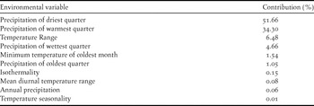
The climatic variables selected for modelling purposes were obtained from the WorldClim database at 1 km2 resolution (http://www.worldclim.org/). To avoid multi-colineality and overfitting in our final models (Peterson Reference Peterson2007), and to obtain an appropriate variable set size for the number of locality points (see Fielding and Bell Reference Fielding and Bell1997), we reduced the original set of 19 climatic variables to 10 (Table 1). We achieved this by assessing the Spearman’s correlation coefficient (rs) for the 19 variables and the 25 locality records, and using this coefficient as a distance measure for a neighbour joining cluster analysis (see Krebs Reference Krebs1989) with 1,000 bootstrap replicates. We first selected all clusters that were separated from the others by a distance < 0.8 and then chose the most distinct variable within each (in terms of its distance from other clusters) to represent the clusters.
Table 1. Heuristic estimates of the relative contribution of individual environmental variables to the definition of a distribution model for the Santa Marta Foliage-gleaner.
To model the ecological niche of the Santa Marta Foliage-gleaner, we used the MaxEnt algorithm for ecological niche modelling (Phillips Reference Phillips2010). In accordance with our sample size, we ran nine distinct models comprising different combinations of three regularisation constants (0.25, 0.5 and 0.8) and linear, quadratic and linear + quadratic features (Phillips and Dudik Reference Phillips and Dudik2008). In all cases, model calibration was based on all available occurrence data (n = 25), with a 1,000 sample point background and an extent restricted to the SNSM at elevations > 400 m. To select among models we used AIC corrected for small sample sizes (AICc) using the model selection tool in the software ENMTools 1.3 (Warren et al. Reference Warren, Glor and Turelli2010).
The selected model was subsequently evaluated using a five-fold cross-validation technique, which is considered appropriate for our sample size (Hastie et al. Reference Hastie, Tibshinari and Friedman2001, Peterson et al. Reference Peterson, Soberón, Pearson, Anderson, Martínez-Meyer, Nakamura and Araújo2011). A total of four runs of the five-fold cross-validation were employed through data reshuffling (Efron Reference Efron1987), producing a total of 20 replicates that could be used to assess uncertainty around estimates of model performance and significance (Hastie et al. Reference Hastie, Tibshinari and Friedman2001, Dormann Reference Dormann2007, Elith et al. Reference Elith, Phillips, Hastie, Dudík, Chee and Yates2011). Model performance was assessed based on regularised training gain values and threshold-based omission error rates on training and test data, whereas model significance was tested using threshold-dependent binomial probability tests (Anderson et al. Reference Andersson, Lew and Peterson2002, Pearson et al. Reference Pearson, Raxworthy, Nakamura and Peterson2007, Phillips and Dudik Reference Phillips and Dudik2008). For this, we used the 10 percentile training presence and 0.9 fixed sensitivity thresholds (see below). We estimated confidence intervals for gain values and omission rates using the mean and standard deviation from the 20 replicates described above, to determine the degree of uncertainty around model performance. Finally, we used jackknife replicates to assess the explanatory power of the 10 environmental variables employed.
Following Peterson et al. (Reference Peterson, Soberón, Pearson, Anderson, Martínez-Meyer, Nakamura and Araújo2011), we used the model calibrated with all 25 geographical records (see above) for projecting the species range and for further analyses requiring geographical projections.
Geographic distribution
The logistic model output from MaxEnt was imported into ArcGIS 9.3 to obtain a predicted geographic distribution based on a grid with 1-km2 resolution. The 10 percentile training presence and the 0.9 fixed sensitivity thresholds (hereafter 10ptt and 0.9fst) were defined to convert the continuous model output into a binary prediction of presence/absence (Peterson et al. Reference Peterson, Soberón, Pearson, Anderson, Martínez-Meyer, Nakamura and Araújo2011). Given the lack of true absence data, we used these two presence-only thresholds to avoid including any measurement of commission error during the subsequent assessment of model performance and significance (Fielding and Bell Reference Fielding and Bell1997, Peterson et al. Reference Peterson, Soberón, Pearson, Anderson, Martínez-Meyer, Nakamura and Araújo2011). These binary predictions were taken as two different estimates of the species occupied distributional area. Following the BAM diagram framework (Peterson et al. Reference Peterson, Soberón, Pearson, Anderson, Martínez-Meyer, Nakamura and Araújo2011), our models were based on the following assumptions: (i) the modelling extent clearly delimits all the potential area that the species could reach through dispersal and there is no geographical barrier limiting its distribution within the study area; (ii) the species is the only Automolus foliage-gleaner in the region and only one other related species is present but at higher altitudes (Thripadectes, treehunters), therefore it is unlikely that any negative interaction with ecologically similar birds could be limiting its geographical range (Pigot and Tobias Reference Pigot and Tobias2013, Claramunt et al. Reference Claramunt, Derryberry, Cadena, Cuervo, Sanín and Brumfield2013).
Ecological distribution
The ecological distribution of the Santa Marta Foliage-gleaner was determined by superimposing the two predictions of its occupied distribution at a 1-km2 resolution (see above) on geographical layers of biomes from 2010, available from the Land-use Planning Geographic Information System of the Agustín Codazzi Geographic Institute of Colombia (http://sigotn.igac.gov.co/sigotn/), and also with digital maps from the Holdridge Life Zones (http://www.fao.org/geonetwork/srv/) and WorldClim layers (see above). Subsequently, we estimated the representation of each biome/life zone within the species range using ArcGIS 9.3.
Extension of occurrence and area of occupancy
We estimated extension of occurrence (EOO) and area of occupancy (AOO) following the IUCN guidelines and compared the resulting values with the threshold values given under criterion B (IUCN 2011) to assess conservation status. EOO was defined as the area inside a convex hull or minimum convex polygon constructed from all 25 occurrences, and since exclusion of discontinuities or disjunctions are discouraged when assessing EOO under criterion B, we did not remove unsuitable habitats for its computation (see IUCN 2011). For the AOO, we estimated two values based on the potential habitat inside our two predictions of the area occupied by the species, by overlapping distributions with rasterised land-cover and ecosystem layers from 2010 using ArcGIS 9.3. Potential habitat was defined taking into account all our observations from 2009 to 2013 and information from Remsen (Reference Remsen, del Hoyo, Elliott and Christie2003) and Krabbe (Reference Krabbe2008). We treat the two AOO values as an interval within which the real AOO is expected to occur.
Population size
To estimate population size, we combined density estimates by elevation and habitat with estimates for the area of each elevational band and habitat within our predicted AOOs. The resulting population estimates were compared with the population threshold given under IUCN criterion C (IUCN 2011). These calculations were based on the assumption that density did not vary across the species’ distribution and thus it should only be considered as a preliminary assessment of population size until density estimates from other parts of the species range are available.
Habitat loss
We calculated the rate of habitat loss by estimating the area for which the original vegetation cover had been transformed within the predicted geographical range. This was carried out by overlapping the AOO projections at 1 km2 with rasterised land-use layers and two additional layers of original ecosystems and biomes (see above).
Representation in protected areas
Taking the AOO projections at 1 km2, we calculated the percentage of the species’ distribution within protected areas by superimposing it on a layer for the National Protected Areas System of Colombia (SINAP; Vásquez-V. and Serrano-G. 2009).
Results
Elevational distribution
Records of Santa Marta Foliage-gleaners came from elevations between 610 m and 1,875 m (Figure 1; Table S1 in the online supplementary material). The lower limit was recorded during the last decade, however, the upper limit originates from two specimen records dating back to 1946. In the last decade the highest record was at 1,560 m.
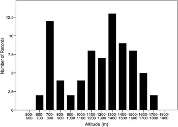
Figure 1. Frequency of observation records for Santa Marta Foliage-gleaners at different elevations in the Sierra Nevada de Santa Marta, Colombia.
Population density estimates
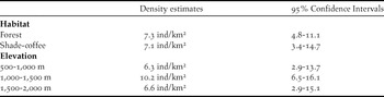
To estimate densities we fitted models including elevation or habitat as factors. There was limited support for a difference in density between forest and shade coffee based on AIC values but there was a clear difference in density by elevation (Table 2). Within the core of the foliage-gleaner’s elevational range (1,000–1,600 m; Figure 1), densities were estimated at 10.2 individuals/km2 (see Table 2).
Table 2. Density estimates (no. Individuals/km2) for Santa Marta Foliage-gleaners in two habitats and within three elevation bands in the Gaira river watershed and on the San Lorenzo ridge, Sierra Nevada de Santa Marta, Colombia.
Ecological niche modelling
Point locality data showed no spatial or sampling bias according to the statistical tests performed. The spatial distribution of point locality data was not significantly different from a random distribution (Z (0.05) = -1.59, P = 0.11), and the permutation tests indicated that locality data were not clumped or over dispersed around human settlements (all P > 0.05, 99% CI = 0.07–0.52). Further, we found no environmental bias among the spatial records, with only four out of 10 climatic variables examined exhibiting spatial auto-correlation (all four P < 0.05).
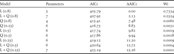
The model using linear features and a regularisation constant (i.e. beta-multiplier) of 0.8 had the lowest AICc value relative to the other eight alternatives (see Table 3). The model selected performed well based on the theoretical parameters used. The mean regularised training gain was 1.15 ± 0.09 (n = 20), while mean values of threshold-based training omission error rates (10ptt = 0.1 ± 0.0001, 0.9fst = 0.04 ± 0.02) and test omission rates (10ptt = 0.19 ± 0.16, 0.9fst = 0.05 ± 0.1) were low. All replicates of the model using different sets of training/test data were highly significant according to the threshold-dependent binomial tests (all P < 0.05).
Table 3. Model set used to choose among three different features (L: linear; Q: quadratic; L + Q: linear + quadratic) and regularisation constants (0.25, 0.5 and 0.8) for modelling the ecological niche of the Santa Marta Foliage-gleaner. Models are ordered according to the AICc value.
Heuristic estimates of the relative contribution of climatic variables to the model were obtained from all jackknife replicates. They indicated that ‘precipitation of the driest quarter’ and ‘precipitation of the warmest quarter’ made the greatest contribution, accounting for a cumulative percentage of 85.95% (Table 1). Similarly, jackknife tests of regularised training gain and test gain showed that the same two variables in addition to ‘annual precipitation’ were important for model construction.
Geographic and ecological distribution
The 10ptt and the 0.9fst were used to obtain two values of the species geographic range defined at a 1-km2 resolution. We interpret these two values, 2,515 km2 and 3,407 km2 respectively, as an interval for the extent of the species occupied distribution. Hereafter, any estimates of areas, rates of habitat loss or percentages are expressed as an interval based on the above areas.
Our model predicted that 88–92% of the range of the Santa Marta Foliage-gleaner was distributed along the north-western and northern flanks of the SNSM between 600 and 2,000 m (Figures 1 and 2), and only 6–10% was above or below this elevational range. Four main biomes (sensu Holdridge Reference Holdridge1963) were represented within the occupied area, of which the Low-Andean and Mid-Andean Orobiomes of Santa Marta accounted for 94–95% of total extent, whereas the Dry-Caribbean and Tropical-Humid Magdalena Zonobiomes comprised less than 6%. The species was largely predicted to occur in areas with mean annual temperatures ranging from 16 to 24°C (97–98% of the extension) and an annual precipitation above 2,500 mm (73–74% of the area), in which rainfall was highly seasonal but temperatures were relatively constant (Figure S1).
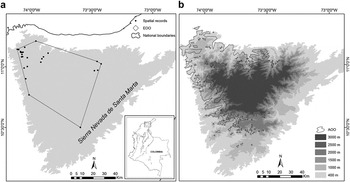
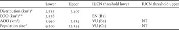
Figure 2. Extension of presence (EOO) and area of occupancy (AOO) of the Santa Marta Foliage-gleaner in the Sierra Nevada de Santa Marta, Colombia. a. EOO estimated as the minimum convex polygon containing all geographical records; b. The projected AOO (at 1-km2 resolution) over an elevational gradient ranging from 400 to 3,000 m.
Extension of occurrence (EOO) and area of occupancy (AOO)
We estimated an EOO of c.3,538 km2 (Figure 2), while our interval for AOO at a resolution of 1 km2 ranged from 1,940 to 2,514 km2 (Figure 2). The EOO estimate and the lower interval of the AOO estimate are below the IUCN thresholds used for threat categorisation under criteria B1 and B2 (see Table 4).
Table 4. Extent of occurrence (EOO), area of occupancy (AOO) and population size estimates for the Santa Marta Foliage-gleaner, with lower and upper thresholds where appropriate. Likely threat categories are presented based on threshold values for the IUCN criteria B and C (see parentheses). Lower and upper estimates are based on the two projections of the species occupied distributional area (see Methods).
* Occupied distributional area. The lower and upper limits correspond to the projected occupied areas obtained from applying the 10 percentile training presence and the 0.9 fixed sensivity thresholds respectively.
** Only one value obtained for the minimum convex polygon based on all spatial records.
^ Population sizes shown here assume an occupation of 50% of the AOO or that at least 50% of the total population correspond to breeding adults (see text).
Population size
Assuming that density is similar throughout the AOO and that all individuals in the population are mature breeding birds, the population size of the Santa Marta Foliage-gleaner could range between c.18,600 and 26,200 individuals, based on our two values for AOO. Under more realistic assumptions, where at least 50% of the AOO is occupied or at least 50% of the total population are breeding adults (see Renjifo et al. Reference Renjifo, Franco, Amaya, Kattán and López-Lanús2002), the estimated population decreases to between 9,300–13,100 individuals. The lower end of this estimation is below the IUCN thresholds for ‘Vulnerable’ under criterion C (Table 4).
Habitat loss and representation in protected areas
According to our estimates, c.23–26% of the area occupied by the species has been subjected to vegetation transformation, with annual and perennial crops and pastures replacing native forests (Figure 3). Along the north-western and western margins of the SNSM, where most records were located (Figure 3), small to moderate-sized agricultural areas and secondary vegetation were relatively common. Records from the southern and north-eastern portion of the massif were near to or enclosed within extensive pastures (Figure 3).

Figure 3. Representation of national and regional protected areas within the area of occupancy AOO (at 1-km2 resolution) of the Santa Marta Foliage-gleaner in the Sierra Nevada de Santa Marta.
Our analysis showed that three national protected areas are inside the estimated AOO of the Santa Marta Foliage-gleaner, covering c.870–1,130 km2 of its extent (44% of the two estimated AOOs; Figure 4). The Sierra Nevada de Santa Marta National Park covered almost the entire northern portion of its AOO, while two other areas covered a small portion within the north-eastern corner of its range: the Jirocasaca Reserve and the Tayrona National Park (at 500–600 m; see Figure 4). No regional or local protected areas were represented in the analysis.
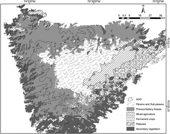
Figure 4. Types of vegetation cover within and around the area of occupancy of the Santa Marta Foliage-gleaner in the Sierra Nevada de Santa Marta.
Discussion
Field data and distribution modelling results show that the Santa Marta Foliage-gleaner is distributed along the most humid flanks of the Sierra Nevada de Santa Marta (SNSM) and is associated with areas of high precipitation and mild temperatures (Figure S1). Both historical and recent records indicate that the species occurs mainly at elevations of 700–1,700 m, but ecological niche models suggest that it could occur a few hundred meters above or below this range (Figures 1 and 2). This species is currently considered as ‘Near Threatened’ (NT; BirdLife International 2014), although there is a lack of quantitative information supporting such a categorisation. While our data require further refinement in order to propose a definitive conservation status, they indicate that the Santa Marta Foliage-gleaner’s distribution and population size are within the criteria for qualifying as a threatened species (see Renjifo et al. Reference Renjifo, Franco, Amaya, Kattán and López-Lanús2002). Indeed, our estimate of extent of occurrence (EOO) qualifies the species as ‘Endangered’ (EN), while our lower threshold estimate for area of occupancy (AOO) and population size support a designation of ‘Vulnerable’ (VU). More positively and contrary to previously published information implying poor representation in protected areas (Krabbe Reference Krabbe2008, BirdLife International 2014), we estimate that national and regional protected areas cover nearly 50% of the species’ AOO.
Modelling considerations
High spatial correlation between locality records can bias distribution models based on environmental niche modelling (Peterson et al. Reference Peterson, Soberón, Pearson, Anderson, Martínez-Meyer, Nakamura and Araújo2011), however, we found no spatial bias among the field data used. Further, we found environmental auto-correlation on just four out of 10 climatic variables and according to jackknife tests none of these variables made a major contribution to model construction. In addition, the usage of two presence-only thresholds instead of one, allowed us to deal explicitly with the trade-off between the spatial extent of the predicted distribution and the inclusion of outlier pixels within it (see Pearson et al. Reference Pearson, Raxworthy, Nakamura and Peterson2007, Peterson et al. Reference Peterson, Soberón, Pearson, Anderson, Martínez-Meyer, Nakamura and Araújo2011), and generate an interval within which the true occupied distributional area of the species probably occurs. Finally, given that there are no apparent physical barriers preventing movement between forested areas within the study region (Figure 3), and that our niche models pointed to environmental and climatic variables as potential factors preventing the species establishment on the drier and more seasonal flanks of the massif, we expect environmental niche models to closely approximate the species’ range.
Population density
The Santa Marta Foliage-gleaner has been considered a relatively rare to locally common bird (Krabbe Reference Krabbe2008, BirdLife International 2014) but there are no published estimates of either density or population size. Here we obtained density estimates that ranged from 6.3 to 10.2 individuals/km2, and their variances indicated that the species could be perceived as rare to common depending on local and elevational variation (Table 2). Our density estimates are slightly higher or within the range estimated for the congeneric Clibanornis rubiginosus (sensu Remsen et al. Reference Remsen, Cadena, Jaramillo, Nores, Pacheco, Pérez-Emán, Robbins, Stiles, Stotz and Zimmer2014), 3–6 birds/km2 at four sites in French Guiana; members of the Automolus genus (A. ochroalemus, 3–4 birds/km2 in French Guiana; A. infuscatus, 3–12 birds/km2 in south-eastern Peru and 9–21 birds/km2 in French Guiana; A. subulatus, 4–7 birds/km2), and even for distant relatives such as Anabacerthia spp. and Phylidor spp. (Remsen Reference Remsen, del Hoyo, Elliott and Christie2003). Elevational variation in density estimates has not been described for any furnarid, yet we have found that density nearly doubled at mid-elevations within the species’ elevation range (between 1,000 and 1,500 m; Table 2). Determining the underlying causes of this variation are beyond this study, but we hypothesise that abundance may be normally distributed across the elevation range, a highly consistent pattern found in different bird communities (e.g. Terborgh Reference Terborgh1971, Reference Terborgh1977).
We did not find differences in density between forest habitats and shade-coffee plantations, potentially reflecting the apparent tolerance of this species to habitat transformation (BirdLife International 2014). However, most individuals in coffee plantations were associated with secondary vegetation bordering streams or in abandoned lots (NB pers. obs.), and the presence of these “habitat features” may allow birds to persist in transformed areas. Nevertheless, it is unknown whether birds would persist in patches of secondary vegetation if they were immersed in a matrix of cattle pastures or sun-grown coffee. Clearly, habitat use and the relative quality of the habitats occupied by the species require further study.
Our estimates for population size ranged from 9,300 to 13,100 individuals, but these values should be treated cautiously given the assumptions on which our calculations were derived. Our estimates are based either on the conservative assumption that (i) 50% of the population were mature breeding adults (see Renjifo et al. Reference Renjifo, Franco, Amaya, Kattán and López-Lanús2002), although in some European passerines breeding adults do not usually comprise more than 40% of the population (e.g. Payevsky and Shapoval Reference Payevsky and Shapoval2000, Wysocki Reference Wysocki2004); or that (ii) 50% of the AOO was occupied at a constant density, when it is unlikely that individuals occupy the full extent of the AOO or at a constant density. Therefore, it is probable that our estimates represent an overestimation of the true population size, and that population size is < 10,000 individuals, which would qualify the species as ‘Vulnerable’ under the IUCN criterion (Table 4).
Elevational distribution
Historically, the Santa Marta Foliage-gleaner has been considered to occur between 700 and 2,100 m (Krabbe Reference Krabbe2008) but records collected since 1950 and in recent years have failed to confirm its presence above 1,800 m. By combining all our field observations with point locality data used for niche modelling, we propose an elevation range of 600–1,875 m. Since our niche model predicts presence close to 2,200 m in elevation, we cannot rule out the possibility that the species may occasionally occur above 2,000 m, but this will require further confirmation.
Geographic distribution
According to our distribution models, the Santa Marta Foliage-gleaner is restricted to the northern and western flanks of the Sierra Nevada de Santa Marta, in north-eastern Colombia. The extent of occurrence (EOO) proposed here was estimated at 3,538 km2, suggesting that the species has a highly restricted range, being lower than the established thresholds for the ‘Vulnerable’ (VU) and ‘Endangered’ (EN) categories under the IUCN criterion B1 (IUCN 2011). The interval for the area of occupancy (AOO) was not entirely consistent with the EOO, but the lower limit was below the VU threshold under criterion B2 (Table 4). Although IUCN strongly recommends estimating the AOO at a 4-km2 resolution, in order to avoid underestimates or obtaining false positives, our analyses were carried out at 1-km2 resolution. We chose this resolution taking into account the highly variable and complex topography of the Sierra Nevada de Santa Marta, where extreme variations in elevation and habitat can occur over small spatial scales, e.g. the Caribbean Sea and the Sierra’s snow-capped peaks (> 5,000 m) are separated by less than 50 km. However, even when estimating AOO at a 4 km2 resolution, its extent did not increase by more than 200 km2 (data not shown).
Conservation status
Our results imply that the distribution of the Santa Marta Foliage-gleaner is smaller than formerly considered (see BirdLife International 2014), and it follows that the species’ ability to respond to potential pressures is more limited than previously thought. The EOO is considered to be a measure of the degree to which any threat is spread spatially across a species’ geographic range (IUCN 2011), and given this species endemism to the north and north-western flanks of the SNSM, any potential threat occurring in this localised region could put the entire species at risk of extinction. Our estimated EOO qualifies the species as ‘Endangered’, and both our EOO and AOO are lower than the distribution size of 4,100 km2 currently listed for the species (BirdLife International 2014).
Large areas of primary forest within the core of the species’ range have been cleared and subject to fragmentation through the establishment of transient and perennial crops, with coffee plantations being the most extensive (Krabbe Reference Krabbe2008, BirdLife International 2014). Despite this, primary forest and old secondary-growth areas maintain a certain degree of connectivity and it is unlikely that dispersal between populations is being severely limited by vegetation transformation. Most of the forest continuity within the foliage-gleaner’s range is associated with the Sierra Nevada de Santa Marta National Park, which alone represents c.40% of the species’ AOO (Figure 4). Previous assessments of potential threats to the species conservation stated that the El Dorado Reserve was the only protected area represented within its distribution (Krabbe Reference Krabbe2008), which clearly is not the case (see Figure 4). The El Dorado reserve and the El Congo biological station are small local reserves whose combined area is probably less than 2–3 km2. The importance of these reserves, however, lies in their location on the north-western corner of the species’ projected AOO (near the Jirocasaca Reserve) where there is a lack of officially designated protected areas (see also BirdLife International 2014). The north-western and western flanks of the SNSM are currently under strong pressure from agricultural expansion (Fundación Pro Sierra Nevada de Santa Marta 1998), and almost all of the unprotected half of the species range is located there (Figures 3 and 4).
Defining an accurate threat category for the Santa Marta Foliage-gleaner would no doubt benefit from additional study of the species’ range and habitat requirements but our results are a valuable quantitative contribution for a future and more robust re-assessment. We used different approximations to evaluate the distribution and population status of this SNSM endemic and our results share common ground: the Santa Marta Foliage-gleaner exhibits a more restricted elevational and geographical range than previous assessments have indicated, meaning that the spatial potential for spreading any possible risk is limited (IUCN 2011). Montane forests along the northern and north-western flanks of the SNSM continue to be transformed and the species is currently present at less than 10 localities (confirmed presence). Taken together, these facts, alongside our estimates for EOO, AOO and population size, strongly suggest that the species could soon be moved to a higher threat category.
It is clear that confirmation of the species’ presence at a variety of localities and at higher elevations is necessary to improve our understanding of its distributional status. Having said that, extensive surveys on the north-eastern and north-western flanks of the SNSM during 2012 did not find birds within an appropriate altitudinal range (CAP pers. obs.). Further, estimates of population density from other localities would greatly assist a more realistic assessment of its population size. Perhaps the most urgent research need is to study the species’ use of space and habitat selection, in order to quantify its habitat requirements and accurately assess its tolerance to vegetation transformation. The Santa Marta Foliage-gleaner is thought to be relatively tolerant to habitat degradation (Krabbe Reference Krabbe2008, BirdLife International 2014), but this is also the case for other threatened SNSM endemics that despite such apparent tolerance, are still being severely affected by forest fragmentation and the loss of connectivity between forest patches at a landscape scale (e.g. Santa Marta Parakeet Pyrrhura viridicata and Santa Marta Bush-tyrant Myiotheretes pernix; Botero-Delgadillo et al. Reference Botero-Delgadillo, Páez and Verhelst2012, Botero-Delgadillo and Olaciregui in press). Other research needs include long-term monitoring programmes capable of tracking the population dynamics of this species and other SNSM endemics (BirdLife International 2014), and also for estimating rates of landscape transformation within the Foliage-gleaner’s range. Finally, immediate conservation actions should target the creation of protected areas or management strategies that protect forests within the western portion of the species range and aim to maintain connectivity between existing forest fragments.
Supplementary Material
The supplementary materials for this article can be found at journals.cambridge.org/bci
Acknowledgements
We want to thank Claudia and Mickey Weber for providing accommodation and logistical support at Hacienda La Victoria in the Gaira watershed. We also thank Santiago Giraldo for his logistical support during fieldwork at the Buritaca watershed. We thank Hernán Arias for undertaking fieldwork in the Buritaca watershed. The associate editor and one anonymous reviewer provided valuable comments on the manuscript. Variable distance transects were carried out in the watershed of the Gaira river and the San Lorenzo ridge as part of the SELVA project ‘Crossing the Caribbean’ financed by the Rufford Small Grants Foundation, Cornell Lab of Ornithology and Environment Canada. Records in the Buritaca watershed were collected under the project “Biodiversity of the Buritaca watershed” financed by FIAAT. Fundación ProSierra and the Department of Biology, Universidad de Los Andes supported PCP-R during field trips to “El Congo” biological station on the north-west flank of the SNSM.


