. . .getting a general-election candidate who can win is the only thing we care about.Footnote 1
—Rob Collins, National Republican
Senatorial Committee
The road to hell is paved with electable candidates.Footnote 2
—Joseph Ashby, conservative blogger
INTRODUCTION
With the rise of the Tea Party and the phenomenon of moderate incumbents “getting primaried,” political scientists and journalists alike have placed added scrutiny on the role of primary elections in our system of representation.Footnote 3 As the first stage of candidate selection, primaries play an important role in choosing the people who will go on to represent voters in Congress. Primary voters exhibit a marked preference for more ideologically extreme candidates (Brady, Han, and Pope Reference Brady, Han and Pope2007; Hall and Snyder Reference Hall and Snyder2013), but general-election voters appear to prefer moderates (Ansolabehere, Snyder, and Stewart Reference Ansolabehere, Snyder and Stewart, III2001; Burden Reference Burden2004; Canes-Wrone, Brady, and Cogan Reference Canes-Wrone, Brady and Cogan2002; Erikson and Wright Reference Erikson, Wright, Brady, Cogan and Fiorina2000). As a stylized fact, primary voters who prefer extreme candidates are thus thought to face a tradeoff between voting for a candidate closer to their views, but less likely to win office, and a candidate farther from their views but perhaps more “electable.” In this article, I study this tradeoff and its consequences for elections and representation in Congress.
How much does the party’s electoral outlook suffer in a district where its primary voters nominate a more extreme candidate, relative to the counterfactual in which the same district nominates a more moderate candidate? If a district nominates a more extreme candidate, how much does the district’s roll-call voting in the next Congress change relative to this same counterfactual—taking into account both the manner in which the extremist would vote and the probability that the extremist wins office? To answer these questions, I combine a scaling technique for estimating candidate positions based on campaign contributions with a regression discontinuity design in U.S. House primary elections, 1980–2010. This strategy allows me to obtain direct counterfactual comparisons between districts with an extreme or more moderate nominee without using assumptions to place districts and candidates on a single ideological scale and without asserting the exogeneity of differences in candidate positions.
I find that the “as-if” random nomination of the extremist candidate causes a substantial decrease in the party’s vote share and probability of victory in the general election. These decreases are large enough to offset the more extreme roll-call voting that extremist candidates offer to primary voters, on average. They are also large enough to offset any other roll-call effects nominating extremists might have, e.g., inducing incumbents to strategically adopt positions like those of extremists. Indeed, the nomination of the more extreme candidate to the general election produces a reversal in observed roll-call voting for the district in the next Congress, on average; that is to say, when a more extreme Democrat is nominated, the district’s roll-call voting in the next Congress becomes more conservative, and vice versa when a more extreme Republican is nominated. In districts that are safe for the party, this reversal disappears. Because even extreme nominees are more likely to win office anyway in safe districts, the effect on downstream roll-call behavior washes out. The tradeoff voters face is therefore variable: in competitive districts they ought to support more moderate primary candidates if they care about winning the office, but in safer districts they have more slack to support extremists.Footnote 4
Overall, however, the nomination of more extreme candidates causes severe damage to the party’s electoral prospects. The nomination of an extremist today makes the party much more likely to lose the general election today, and because of the incumbency advantage, the opposing party is much more likely to win the election again two years later, and four years later, and on. As I show, the nomination of the extremist continues to cause an equally large electoral penalty as far as eight years down the line—the farthest increases in voter information because of redistricting. The decisions that primary voters make in the current election cycle echo many years later.
The article is organized as follows. In the next section, I discuss the theoretical perspectives and expectations motivating the research. Following that, in the third section I provide an overview of the data and empirical strategy used to analyze primary and general elections in the U.S. House, 1980–2010. In the fourth section, I analyze general-election outcomes. In the fifth section, I examine the effect as I sharpen the contrast between extreme and more moderate primary candidates. In the sixth section, I analyze the overall effects on legislative behavior and explore the varying tradeoff that primary voters face between “electability” and ideology. In the seventh section, I study the long-term effects of extreme nominees, showing how the electoral penalty (and its accompanying roll-call effect) persists even four terms—eight years—later. In the eighth section, I briefly consider possible causal mechanisms. Finally, I conclude by discussing the implications of the findings.
THEORETICAL PERSPECTIVES
Primaries are a key part of the American electoral system. By selecting especially partisan candidates, primaries may contribute to the large and growing polarization of U.S. legislatures.Footnote 5 This growth has been especially marked in recent elections, including in those studied in this article, namely, U.S. House elections, 1980–2010. In primaries like these, as the epigraph hinted, parties and their voters must weigh issues of party brand and ideological “purity” against “electability”—the likelihood of a potential nominee winning the general election.Footnote 6 To understand the possible consequences of primary-election results, we must first understand the electoral costs or gains of nominating more or less ideologically extreme candidates. Only then can we assess the potential tradeoffs at play during the primary election.
While primary candidates may be more or less extreme, we have reasons to believe that the candidates that enter primaries are already polarized. Within a primary, some candidates will be farther to the right or left than others, but even the right-most Democrat is likely to be quite left of the left-most Republican in the opposite primary (see for example Bafumi and Herron Reference Bafumi and Herron2010). As a result I will refer throughout the article to “relative moderates” and “extremists”—candidates in a primary who are moderate or extreme relative to their primary opponents, but who likely lie all to one side of the district’s median voter. Classifying primary candidates in this way clarifies our expectations about the consequences of nominating more or less extreme candidates. Even if general-election voters reward nominees who are moderate relative to their primary opponents, polarization may still be high if the pool of candidates as a whole is quite polarized.Footnote 7 Thus in studying the effects of nominating extremists we will learn about one important potential mechanism through which primaries can affect polarization—through the selection of candidates to stand in the general election—but we must be aware that primaries can still affect polarization in other ways, e.g., through affecting the pool of candidates that enter primary elections in the first place.
Considering the overall consequences of nominating extremists is important for the reasons above, but so, too, is studying the way these consequences vary across districts. We might suspect, for example, that any reaction of general-election voters will be muted in especially partisan districts. In these “safe” districts, general-election voters may be likely to elect their party’s nominee regardless of her ideological position relative to her primary opponents. This is an important source of variation because many U.S. House districts are safe, by typical standards. In the 2008 presidential election (the last such election occurring within the period of study), for example, almost exactly half of all Congressional districts had a Democratic presidential vote share above 0.6 or below 0.4. Primaries are likely to play a different role in these districts than in the other half of the districts which are more competitive. In addition to the overall on-average effect of extremist nominations—our single most important quantity of interest—we should therefore also investigate variation in the effect across safe and competitive districts in order to gain further understanding of where and when extremists are punished more or less in the general election.
The effect might vary, also, with the presence of an incumbent candidate. Incumbents possess a large electoral advantage (e.g., Erikson Reference Erikson1971; Gelman and King Reference Gelman and King1990) which may give them leeway to take different positions. If incumbents are more likely to be relatively moderate primary candidates, then any penalty to candidates labeled more “extreme” might actually be driven by the removal of the incumbent when the extremist wins nomination and not by any other characteristic of the more extreme candidate. This is one reason to investigate the effect in open-seat races, where neither primary has an incumbent running. A second reason is that most incumbents first enter office through open-seat races. Given the well-known persistence of incumbents once in office, open-seat primaries are especially important for selecting candidates.
Short-term electoral outcomes are not the only consequence of nominating extremists in primary elections, either. Even if an extremist performs poorly in the general election, her nomination might be valuable to her supporters in other ways. The podium that the general-election campaign offers might allow an extremist to trumpet her views and incite support for future election cycles, and the views she espouses might make their way into the legislature even if she, herself, does not. This could occur directly through increased demand for her supported policies or indirectly through the threat her candidacy signals to the incumbent anticipating future elections (see for example Sulkin Reference Sulkin2005). For these reasons it is important to study not just the immediate electoral consequences of nominating more or less extreme candidates, but also the effects of nominating relatively extreme or moderate candidates on downstream roll-call voting.
In similar ways, extremist nominees might also affect downstream election results. On one side, advocates and others often point to the “galvanizing” effect of extremist nominations. Even if the extreme nominee loses in the general, the logic goes, she can succeed in energizing the party’s base, which can enhance the party’s electoral fortunes the next time around. After losing her Senate election, Tea-Party candidate Christine O’Donnell, for example, declared that “Our voices were heard and we’re not going to be quiet now. . .. This is just the beginning.”Footnote 8
On the other side is the cold, hard logic of the incumbency advantage. Incumbents in the U.S. House enjoy enormously high reelection rates (e.g., Jacobson Reference Jacobson2012), and the “as-if” random assignment of incumbency status conveys a roughly 40 percentage-point increase in the probability the party retains the seat in the next election cycle (Lee Reference Lee2008). Once a party controls a seat, it is unlikely to give it up for a long time. Fowler and Hall (Reference Fowler and Hall2013), for example, show that the election of a Democrat over a Republican in a coin-flip election today makes the district more likely to still be represented by a Democrat 16 years later. The decision to nominate the extremist in the current primary election thus might boost the opposing party’s downstream electoral outcomes if it makes that party more likely to gain incumbency status today.
Finally, we can learn more about the candidate selection process, and can speak to formal models of these processes, by studying the mechanisms underlying the effects of extremist nominations. The electoral effects of nominating extremists might result from their ideological positioning, as implied by spatial models of electoral processes (Downs Reference Downs1957), or they might result from other differences between the two types of nominees. Probabilistic voting models often predict, for example, that candidates will strategically take more extreme positions when they are disadvantaged on a separate dimension of valence such as quality (e.g., Ansolabehere and Snyder Reference Ansolabehere and Snyder2000; Aragones and Palfrey Reference Aragones and Palfrey2002; Groseclose Reference Groseclose2001). Models of these forms also suggest comparative statics in which increases in the information about candidate positions lead to larger disadvantages for extreme positions, suggesting another dimension of variation in the response to extremist nominees.
In this section, I have explained why considering the effects of extremist nominations is important and I have situated the study in the context of legislative polarization. I have also described how I operationalize “extremist” primary candidates—those who are ideologically extreme relative to their primary opponents—and offered some important theoretical sources of variation in the consequences of nominating these relatively extreme candidates. I have also laid out theoretical ideas for testable mechanisms underlying the response to extremist nominees. With these in mind, I now proceed to describe the details of the empirical approach and its results.
EMPIRICAL APPROACH
Primary-Election Campaign Contributions Predict Candidate Ideology
For information on classifying candidates as extremists, I rely on the estimated ideological positions of U.S. House primary candidates from Hall and Snyder (Reference Hall and Snyder2013), which covers the years 1980–2010.Footnote 9 Technical details on the method are available in Appendix B. Candidates are scaled on the basis of their primary-election campaign receipts,Footnote 10 imputing each candidate’s ideological position from the contribution-weighted average estimated positions of her donors.Footnote 11 The donors’ positions are estimated as the contribution-weighted average DW-NOMINATE score (Poole and Rosenthal Reference Poole and Rosenthal1985) of incumbents they have donated to, but excluding donations to candidate i when computing the score for each candidate i. The technique is similar to those employed in, for example, Bonica (Reference Bonica2013) and McCarty, Poole, and Rosenthal (Reference McCarty, Poole and Rosenthal2006). I choose this technique over other options only because it produces scalings that are specific to the primary election. Using general-election contributions—though statistically efficient for many other purposes—would introduce post-treatment bias in the present setting since the “treatment,” the nomination of the extremist, occurs prior to the start of the general-election campaign.
To validate this scaling technique in the sample used for analysis, Figure 1 compares it to observed DW-NOMINATE scores for primary candidates who go on to win the general election. The donor-based scaling of candidates correlates with observed DW-NOMINATE scores at 0.90.Footnote 12 This is consistent with a fuller battery of validation tests presented in Hall and Snyder (Reference Hall and Snyder2013). As a result, there is good reason to believe that the estimated primary candidate positions are reflective of their actual ideological positioning. Importantly, any random error in these estimated positions biases the subsequent analysis against finding differences in outcomes for more and less extreme candidates.Footnote 13
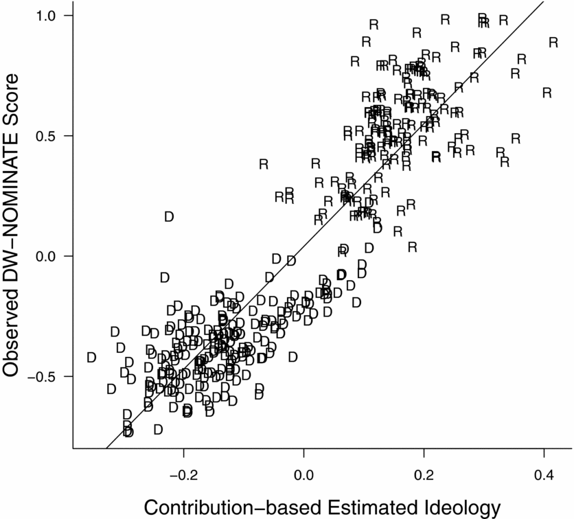
FIGURE 1. Estimated Ideology of Primary Candidates and Observed Roll-Call Behavior
In primary races with two major candidates, the race is tentatively identified as being between an extremist and a relatively moderate candidate if the difference between their estimated ideological positions is at or above the median in the distribution of ideological distances between the top two candidates in all contested primary elections. This median distance translates to roughly one-third the distance on the DW-NOMINATE scale between the medians of the two parties in the 112th Congress, and it is approximately two to three times as large as the average distance between representatives and their own party’s median.Footnote 14 These are therefore races between candidates who offer meaningfully different platforms within the umbrella of their party.
Using a strong cutoff like this has two potential advantages. First, it may reduce the number of incorrect moderate/extreme labels caused by measurement error in the donor scores. Second, it ensures that we are focusing on strong comparisons in which the two primary candidates are starkly different.Footnote 15 After presenting main results, I address the use of this cutoff, showing how the results are robust to alternate definitions and, moreover, that changes in the estimates as the cutoff is changed accord with theoretical predictions—namely, that the effect grows in magnitude as the cutoff becomes more extreme (as the contrast between the two candidates sharpens).Footnote 16
Dataset Covers U.S. House Elections, 1980–2010
Data on U.S. House primary and general elections are compiled from primary sources by Ansolabehere et al. (Reference Ansolabehere, Hansen, Hirano and Snyder2010). I focus on elections in the years 1980–2010 to match the data on candidate positions. I keep all primary elections in which at least two candidates have donor scores.Footnote 17 Among these elections, I analyze the two candidates with the top two vote totals, and I calculate each candidate’s share of the top two vote totals.Footnote 18 Full summary statistics are available in Appendix A in Table A.1.
What Kind of Elections Enter the Sample?
The analysis uses a special subset of all primary elections—namely, contested primaries with two “viable” candidates who raise enough money to allow for reliable ideological scaling. Investigating the characteristics of this sample is important for understanding and interpreting the results.
Table 1 breaks down the primary elections that enter the sample according to the presence of incumbents and the safety of the district for the party holding the primary. Districts are defined as “safe” if the party’s share of the presidential two-party normal vote, calculated as the average presidential vote share for the redistricting period, is above 60%.Footnote 19 As the first row shows, the majority of observations (287 of the 504 total) occur in primaries for races with no incumbents present, i.e., no incumbents in either party’s primary. Of these 287 races, roughly 35% occur in districts that are safe for the party holding the primary, with the lion’s share of the remainder occurring in “competitive” districts, those where the party’s presidential normal vote is below 60% (or, equivalently, those where the Democratic presidential normal vote is between 40% and 60%).
TABLE 1. Number of Primary Elections In Sample, By Type: U.S. House, 1980–2010
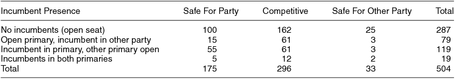
Note: The majority of races occur in open seats either in competitive districts or districts that are safe for the party.
Looking across the columns, we also see that the majority of primary races in the sample occur either in districts safe for the party (175 total) or in competitive districts (296). It is unusual for a primary election that occurs in a district safe for the other party to enter the sample. This is probably because these primaries are unlikely to yield viable candidates, and thus are unlikely to be competitive or to feature sufficient contribution behavior to scale candidates. In the Appendix, I compare these characteristics to those of the larger universe of all primary elections. The districts that enter the sample are no different in terms of their partisanship, but they are disproportionately open-seat races.
Estimation Strategy: Regression Discontinuity Design in Primary Elections
I estimate equations of the form
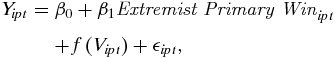 \begin{eqnarray}
Y_{ipt} &=& \beta _0 + \beta _1 \mathit {Extremist \ Primary \ Win}_{ipt}\nonumber\\
&& +\, f(V_{ipt}) + \epsilon _{ipt},
\end{eqnarray}
\begin{eqnarray}
Y_{ipt} &=& \beta _0 + \beta _1 \mathit {Extremist \ Primary \ Win}_{ipt}\nonumber\\
&& +\, f(V_{ipt}) + \epsilon _{ipt},
\end{eqnarray}
where $\mathit {Extremist \ Primary \ Win}_{it}$
is an indicator variable for the extremist winning party p's primary in district i at time t. Thus β1 is the quantity of interest, the RDD estimator for causal effects from the “as-if” random assignment of an extremist in the general election.Footnote
20
The variable Yipt
stands in for three main outcome variables: party vote share, party victory, and the DW-NOMINATE score of the winning general-election candidate in the ensuing Congress. The term f(Vipt
) represents a flexible function of the running variable, the extremist candidate’s vote-share winning margin, i.e., the extremist candidate’s share of the top two candidates’ vote less 0.5, which determines treatment status. I present estimates using a variety of specifications for f as well as at different bandwidths, following the usual RDD practices (Imbens and Lemieux Reference Imbens and Lemieux2008). Typically, f either contains a high-order polynomial of the running variable or a local linear specification estimated separately on each side of the discontinuity.Footnote
21
$\mathit {Extremist \ Primary \ Win}_{it}$
is an indicator variable for the extremist winning party p's primary in district i at time t. Thus β1 is the quantity of interest, the RDD estimator for causal effects from the “as-if” random assignment of an extremist in the general election.Footnote
20
The variable Yipt
stands in for three main outcome variables: party vote share, party victory, and the DW-NOMINATE score of the winning general-election candidate in the ensuing Congress. The term f(Vipt
) represents a flexible function of the running variable, the extremist candidate’s vote-share winning margin, i.e., the extremist candidate’s share of the top two candidates’ vote less 0.5, which determines treatment status. I present estimates using a variety of specifications for f as well as at different bandwidths, following the usual RDD practices (Imbens and Lemieux Reference Imbens and Lemieux2008). Typically, f either contains a high-order polynomial of the running variable or a local linear specification estimated separately on each side of the discontinuity.Footnote
21
The key identifying assumption of the RDD is that potential outcomes are smooth across the discontinuity, i.e., that districts where the relatively moderate primary candidate barely wins (or, equivalently, those where the extremist candidate barely loses) are in the limit comparable to those in which the relative moderate barely loses (or, equivalently, those where the extremist candidate barely wins). Assumptions of “no sorting” like this have been challenged in the context of general-election U.S. House races (Caughey and Sekhon Reference Caughey and Sekhon2011; Grimmer et al. Reference Grimmer, Hersh, Feinstein and Carpenter2012; Snyder Reference Snyder2005), but across numerous other electoral contexts are found to be highly plausible (Eggers et al. Reference Eggers, Fowler, Hainmueller, Hall and SnyderN.d.).
For primary elections, this assumption is extremely plausible; to sort, candidates would need to have precise information about the expected outcome of primary elections, and would need to exert extra effort only after finding out that the election was going to be extremely close.Footnote 22 Given the difficulty even general-election campaigns have in predicting votes (Enos and Hersh N.d.), and the typical “running scared” mentality that leads candidates to pull out all the stops (King Reference King1997), this seems unlikely. In addition, I validate the assumption in the Appendix by presenting balance tests using the same samples and specifications as the main results in the article. No evidence of sorting is found.Footnote 23
In addition to testing for sorting, it is also important to show that the RDD estimate is not sensitive to choices over the size of the bandwidth and the functional form of the running variable's specification. In the Appendix, I replicate the main analysis on general-election outcomes at a large variety of bandwidths and specifications and show that the resulting estimates consistently produce the same conclusion.
One final aspect of the estimation strategy deserves mention. Like any comparison across candidate types, the RDD I employ measures the total effect of assigning the extremist vs. the relatively moderate candidate to the general election. This includes the component of the overall effect that comes from the change in ideology, but also includes any other factors that differ between the two types of candidates.Footnote 24 To understand the consequences of primary voters’ decision to nominate one kind of candidate or the other, though, we want to include all of the differences between the two types of candidates, not only their ideological differences. For the present analysis, then, this feature of the estimation strategy is suitable. However, it is also valuable to understand why the observed effects occur. To make progress in this direction, I examine heterogeneity in the effect across contexts as well as characteristics of the more moderate and more extreme bare-winners after presenting the main results.
RESULTS: EXTREMIST NOMINEES PERFORM WORSE IN THE GENERAL ELECTION
Figure 2 plots the discontinuity in the data. As can be seen, when the extremist goes from barely losing the primary to barely winning it (horizontal axis), the party’s general-election vote share decreases noticeably. Among “coin-flip” primary elections between a relative moderate and an extremist, the nomination of the extremist appears to cause a large decrease in the party’s general-election vote share.
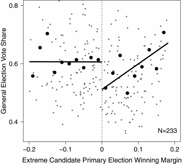
FIGURE 2. General-Election Vote Share After Close Primary Elections Between Moderates and Extremists: U.S. House, 1980–2010
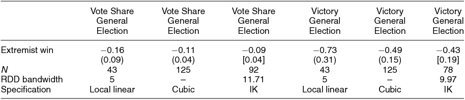
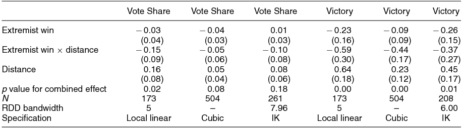
Table 2 presents the estimates from Equation 1 using general-election vote share and victory as the outcome variables, with three specifications for each. In the first and fourth columns, I use a 5% bandwidth and a local-linear specification of the forcing variable, estimated separately on each side of the discontinuity. In the second and fifth columns, I use all the data and include a cubic specification of the running variable. In the third and sixth columns, I employ the “optimal bandwidth” procedure from Imbens and Kalyanaraman (Reference Imbens and Kalyanaraman2012).Footnote 25
TABLE 2. RDD Estimates of the Effect of Nominating an Extreme Candidate on General Election Vote Share, U.S. House 1980–2010
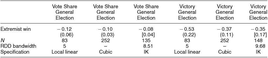
Notes: Maximum of robust and conventional standard errors in parentheses. Columns 3 and 6 use optimal bandwidth technique from Imbens and Kalyanaraman, implemented using rdob in Stata. Standard errors from this procedure in brackets.
As the table shows, the “as-if” random assignment of the extremist to the general causes approximately a 8–12 percentage-point decrease in the party’s share of the general-election vote, and a 35–53 percentage-point decrease in its probability of victory. These are large effects.
These estimates average over the different types of primaries, including those for open-seat races as well as incumbent-held seats and districts that are safe, competitive, or unsafe for the party holding the primary. As discussed in the “Theoretical Perspectives” section, investigating the variance in the effect across these district types is important for interpreting it. In Figure 3, I plot RDD estimates of the effect of nominating the extremist on the probability the party wins the general election, estimated separately for three relevant sets of elections. For comparison, the first estimate, labeled “Overall,” corresponds to the overall estimate from the fifth column in Table 2.
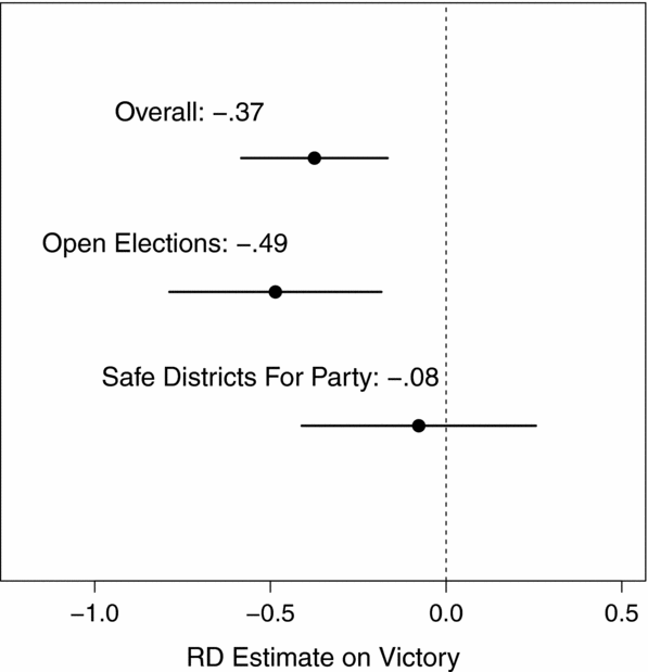
FIGURE 3. Effects of Nominating the Extremist Candidate on General Election Victory Across Primary Types
The second estimate uses only open elections, i.e., elections with no incumbent present in either primary. For these elections the effect is approximately 12 percentage points larger in magnitude than the overall estimate.Footnote 26 Open-seat races appear to be doing most of the work in driving the observed penalty to extremists, either directly because these races feature no incumbents or because of other factors that differ across districts that tend to have open-seat races and those that do not. Whatever the reason, this large effect shows that incumbents, or the loss of the incumbency advantage when relatively moderate incumbents lose to more extreme candidates, cannot explain the findings.Footnote 27
Finally, the third estimate uses only primaries that occur in districts that are safe for the party holding the primary, i.e., districts where the presidential normal vote is at or above 60% for the party. Here we find almost no penalty to nominating the extremist, perhaps because the partisan voters in the district support whomever the party nominates.Footnote 28 As mentioned in the theoretical section, a large number of districts are safe for one party or the other in U.S. House elections. The tradeoff between “electable” and “ideologically pure” candidates is quite different in these districts, as this heterogeneity in the effect shows.
This section has established the electoral penalty that the party faces when it is “as-if” randomly assigned an extremist candidate for the general election. This penalty is large, probability of victory and it is especially driven by the reactions of general-election voters in open-seat races. The penalty to extremists largely dissipates in districts that are safe for the party.
INCREASING EFFECT SIZE ACROSS CANDIDATE EXTREMISM
The results presented thus far average over treatments of varying intensity because the ideological distance between the relatively moderate and extreme candidate in contested primaries is not constant across races. To ensure that I only include true contrasts between an extremist and a more moderate candidate, the analysis above employed the median ideological distance between primary candidates as the cutoff for inclusion in the sample. By examining the effect across possible sizes of this cutoff, we can test the theoretical expectation that the electoral penalty should increase as the distance gets larger, and we can verify the robustness of the findings.
There are two methodological reasons to prefer larger cutoffs. First, too small of a cutoff might increase the probability of misclassifications due to measurement error in the donor scores. Measurement error in these scores means that, for candidates closer together in ideology, there is a greater probability that by random chance the more extreme candidate appears to be more moderate than the relatively moderate candidate. This type of error would lead to measurement error in the treatment variable—by identifying a winning candidate as an extremist and thus incorrectly calling the district “treated,” or, likewise, by calling her more moderate and incorrectly calling the district a “control” district—and thus would lead to attenuation bias in the estimates. At larger cutoffs this concern may be mitigated because two very far apart candidates are less likely to be misclassified in this manner.
Second, smaller cutoffs also bring into the sample more elections in which the contrast between the “moderate” and the “extremist” is less than sharp. Given the low information of voters, there is surely a point at which the distance between the candidates ceases to matter, and so the distinction between “treated” districts and “control” districts among these primaries becomes moot. Again, at larger cutoffs this concern dissipates.
Despite these advantages, there is also a cost to this cutoff approach. Although the treatment is “as-if” randomly assigned in the RDD, the intensity or “dose” of the treatment is not. Cutting the sample based on intensity can provide a sense of how the effect varies with intensity, but it may also indicate underlying differences in the kinds of districts that have greater or smaller ideological distances between primary candidates. To address this problem, I have also estimated effects including all races in the sample, without employing a cutoff on ideological distance, and including a control for the estimated ideological distance between the candidates as well as an interaction of this distance with the treatment variable. The results, available in Table A.6, are consistent with those presented in the article.
Figures 4 and 5 present RDD estimates for the effect of nominating the extreme candidate over the more moderate candidate on the party’s general-election vote share and probability of winning across possible cutoffs. The horizontal axis represents the cutoff value used, and the 25th, 50th, 75th, and 95th percentiles of the distribution of ideological distances among closely contested primary elections are indicated towards the bottom of the plots. Vertical lines represent 95% confidence intervals from robust standard errors. The estimates reported in the previous sections are highlighted and indicated in the plot with arrows.
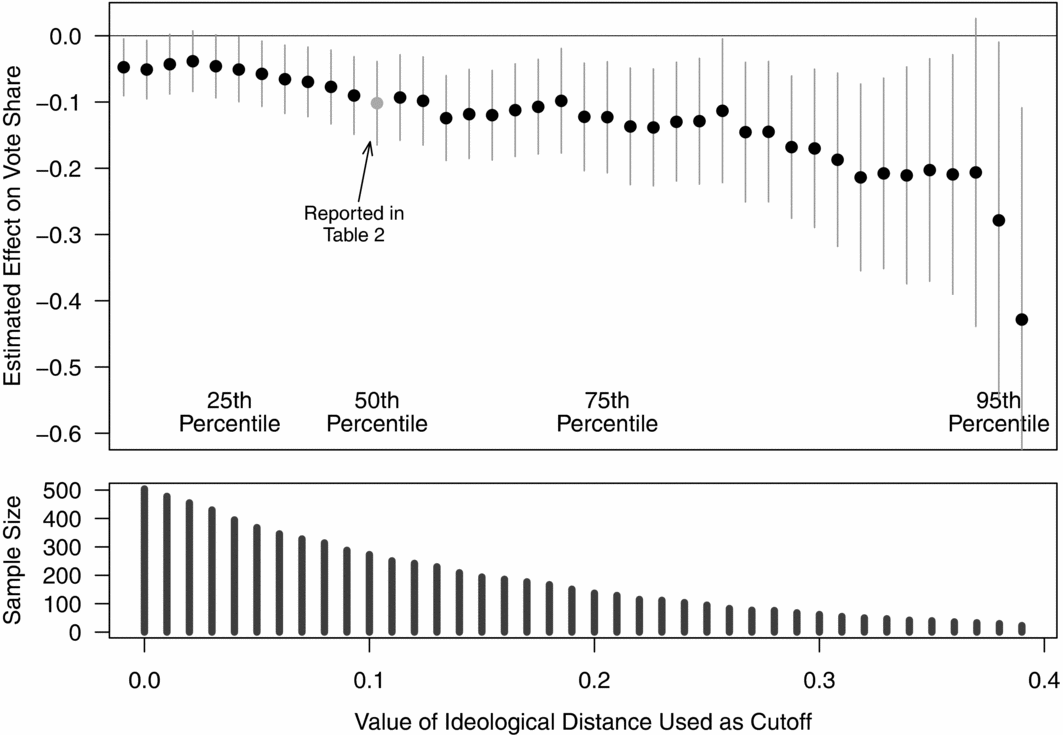
FIGURE 4. Estimate of Effect on General-Election Vote Share Across Possible Cutoffs
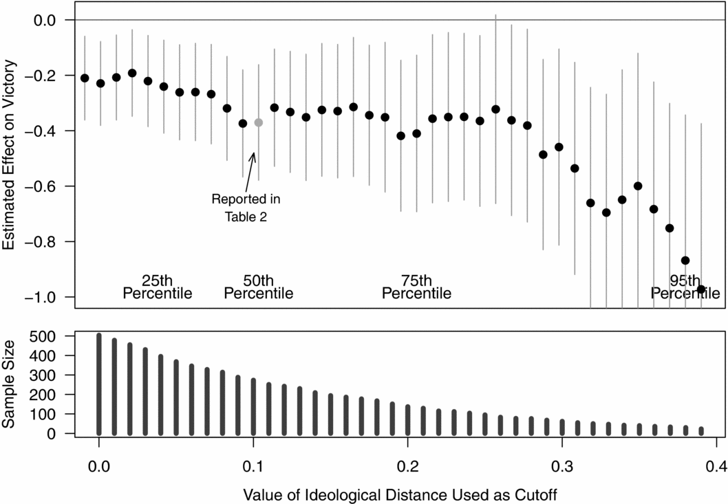
FIGURE 5. Estimate of Effect on General-Election Victory Across Possible Cutoffs
As the figures show, we find similar, negative estimates even when we include all comparisons between extremists and relative moderates (when the cutoff is zero in the figures). As expected, the estimates grow in magnitude as the cutoff increases. In both cases, the estimated effect more than doubles if the 95th percentile is used as the cutoff—i.e., only using the most extreme cases—relative to the 50th percentile cutoff used in the previous section.Footnote 29
In contested primary elections, the nomination of an extreme candidate causes a large decrease in the party’s electoral prospects in the general election. This effect is present in many settings and especially large in cases in which the extreme candidate is especially ideologically extreme. Having established this on-average electoral penalty, we can examine its consequences for behavior inside the legislature.
EFFECTS ON ROLL-CALL VOTING IN CONGRESS
In this section, I link the nomination of an extremist candidate to roll-call voting in the subsequent Congress. As the “Theoretical Perspectives” section discussed, extremist nominations could affect roll-call voting directly, by affecting which candidate and which party attain office, and indirectly, by altering the incentives of those in office.
Two opposing forces compose this first, “direct” effect. On the one hand, the nomination of an extreme candidate pulls subsequent roll-call voting away from the middle and towards the party’s ideological core—to the left when Democratic extremists are nominated and to the right when Republican extremists are—because the extremist is likely to vote more extremely if elected. On the other hand, as the previous section showed, the nomination of the extremist benefits the opponent party in the general, making roll-call voting more likely to shift in the other party’s direction—to the right when Democratic extremists are nominated, and to the left when Republican extremists are.
Figure 6 suggests this dynamic in Democratic and Republican primaries, respectively. The horizontal axis represents the estimated donor score of the winning primary-election candidate, and the vertical axis represents the DW-NOMINATE score of the winning general-election candidate in the ensuing Congress. Points are labeled “R” if the Republican candidate won the general election, and “D” if the Democrat did. Consider the left panel, representing Democratic primaries. In the elections with a relatively moderate Democratic primary winner—observations to the right of the plot—subsequent roll-call voting tends to be liberal (negative on the DW-NOMINATE scale). As we move to the left, i.e., as the winning Democratic primary candidate becomes more extreme, average roll-call voting first becomes more liberal, because the primary winner delivers more liberal roll-call voting. However, as the donor score becomes more extreme, Republicans begin to gain a more significant electoral advantage, and roll-call voting starts to become increasingly conservative.
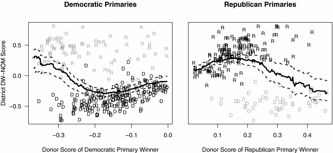
FIGURE 6. Nominee Ideology and Roll-Call Voting
The same pattern is present in the Republican primaries. Moderate primary winners—those to the left of the plot—tend to win and deliver moderate roll-call voting. As we move to the right, there is an increase in roll-call conservatism, but as we move farther right, this effect is washed out by the increasing electoral victories of Democrats in the general election.
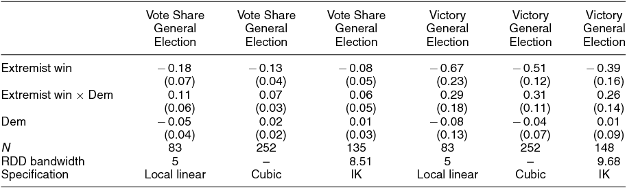
As previewed in the “Theoretical Perspectives” section, the tradeoff between extremist and more moderate nominations may vary across districts. To explore this, as well as to add empirical rigor to the descriptive data presented above, I re-estimate the RDD with the district’s subsequent DW-NOMINATE score as the outcome variable. Overall, I find that the nomination of the extremist causes a reversal in roll-call voting, producing more conservative roll-call voting when Democrats nominate a more extreme candidate and more liberal roll-call voting when Republicans nominate a more extreme candidate (see Figure 8 in the next section). Here, I interact the treatment variable with an indicator for whether the district is safe for the party holding the primary.
The first three columns of Table 3 investigate the effect in Republican districts. The coefficient on “Extremist Win” reflects the effect of nominating the extremist in districts that are not safe for the party (when “Safe For Party” is zero). Here we see that nominating the extremist produces a leftward shift in roll-call voting. Though the sample sizes make the estimate somewhat unstable, it is consistently negative and substantively meaningful. In all three cases, moreover, we see that this roll-call reversal disappears in safe districts, where the electoral penalty to nominating the extremist is small.
TABLE 3. RDD Estimates of the Effect of Nominating an Extreme Candidate on District’s Roll-Call Representation, U.S. House 1980–2010
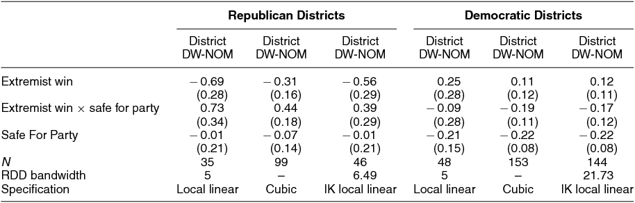
Note: Maximum of robust and conventional standard errors in parentheses. Third and sixth columns select optimal bandwith from Imbens-Kalyanaraman and apply with local-linear OLS.
Consider, for example, the second column, which includes all of the data. In districts that are not safe for the party, nominating the extremist is estimated to cause a − 0.31 point decrease in the DW-NOMINATE score of the representative voting on behalf of the district in the next Congress. In safe districts, on the other hand, this effect is estimated to be positive 0.13 ( − 0.31 + 0.44 = 0.13), and we can reject the null hypothesis that the effect is the same across these two cases. The same pattern of evidence, though noisier, occurs in Democratic districts, as shown in the latter three columns of the table. In competitive districts, nominating the extremist appears to cause more conservative roll-call voting, but the effect moves close to zero in districts that are safe for the party.
The previous section demonstrated that there is a pronounced electoral penalty to nominating an extreme candidate over a more moderate candidate in contested primaries. It is difficult to evaluate the implications of this penalty for primary voting behavior without considering the overall effects nominating an extremist produces. This effect is in part a composite of the electoral penalty and the differential roll-call behavior of the extremist vs. the general-election candidate of the other party.
As it turns out, the implications vary depending on district conditions. In competitive districts, the nomination of an extremist may be a “mistake” from the point of view of primary voters who care about average roll-call representation in the legislature. In these districts, the likelihood that the other party will defeat the extreme nominee is too large, and the desired roll-call voting of the extremist nominee too unlikely to manifest itself in the legislature. But in safe districts, this may no longer be the case. In safe districts, the extremist wins enough of the time to make the observed roll-call effect close to zero.
It is more difficult to evaluate the possible “indirect” effects nominating the extremist has on roll-call voting, but the results place some bounds on them. That roll-call voting shifts in the opposite direction in competitive districts tells us that these indirect effects cannot be large relative to the change in roll-call voting caused by switching the party of the representative. It is still possible that the nomination of the extremist could cause incumbents in the district in the future to adopt more extreme positions, but any such effect must be small relative to the direct effects from nominating the extremist that flow through the changes in the probability the party wins the seat.
EXTREMIST NOMINEES AFFECT FUTURE ELECTIONS
On average, the nomination of an extremist has a pronounced negative effect on the short-term electoral fortunes of the party. What are the longer-term effects of this nomination? The “Theoretical Perspectives” section laid out arguments for either a “galvanizing” effect, in which nominating the extremist today might help the party tomorrow even if it loses today, or for a sustained penalty brought on by the likelihood of ceding incumbency status to the opposite party.
Consistent with this latter view, Figure 7 presents estimates from Equation 1 using the party’s victory and vote share in subsequent electoral cycles as the dependent variable.Footnote 30 As the figure shows, the nomination of an extremist today continues to cause an equally large decrease in the party’s expected probability of victory and vote share even four terms, or eight years, later—the farthest downstream that redistricting allows us to examine.
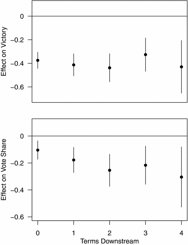
FIGURE 7. Long-Term Effect of Nominating Extremist on Party’s General-Election Victory and Vote Share
Figure 8 plots the same for the district’s downstream DW-NOMINATE score, separately for Democratic and Republican primaries, pooling over safe and competitive districts. The overall reversal explored in the previous section persists even four terms (eight years) later. In Democratic districts, roll-call voting becomes more conservative (increases) on average, and in Republican districts it becomes more liberal. Like in the previous section, this suggests that any indirect effects of extremist nominations on roll-call voting are small. Though extremists might be able to pull future roll-call voting towards their preferred positions without serving in office, any such effect is swamped in the long run (as well as the short run) by the direct effects of nominating the extremist and giving the office to the other party.
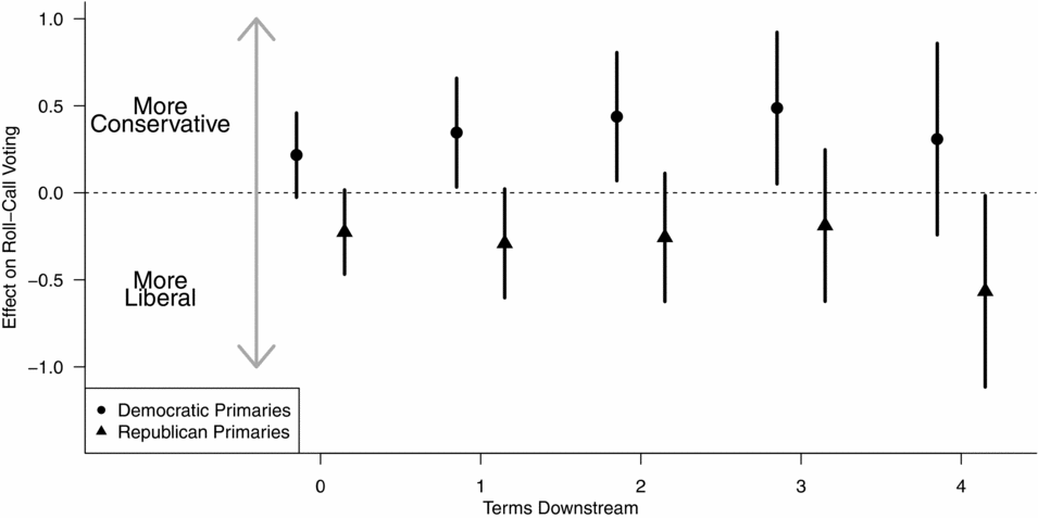
FIGURE 8. Long-Term Effect of Nominating Extremist on District’s Roll-Call Representation
The decisions that primary voters make affect the current election. As I have shown, their choice influences the party’s vote share and probability of victory, as well as the style of representation they receive in Congress. But the decisions primary voters make today echo for at least the next decade, too.
DISCUSSION OF POSSIBLE MECHANISMS
How do we account for these effects? In this section I consider a variety of explanations and mechanisms, focusing both on the “bundle” of characteristics that extremists and moderates offer and on other features of the electoral environment. These explanations are not mutually exclusive, nor do they comprise the whole universe of possible explanations, but they do encompass some of the most salient possibilities.
Extremists Do Not Differ On Observable Valences
Perhaps the most obvious possible mechanism other than ideological positioning is that extremist nominees may possess some kind of valence disadvantage relative to more moderate candidates, as discussed previously.Footnote 31 Although measuring “valence” directly is impossible, we can assess whether bare-winner extremists appear to differ from bare-winner moderates in their previous office-holder experience, a measure often used as a proxy for unobserved quality and known to provide a valence advantage (Jacobson Reference Jacobson1989, Reference Jacobson2012).Footnote 32
The first point estimate in Figure 9 reports the RDD estimate like in Equation 1, but where the outcome is an indicator for whether the winning primary nominee has previous office-holder experience. This tests the hypothesis that part of the “treatment” of nominating the extremist candidate is receiving a nominee with more or less quality, in a particular sense, than the “control” of nominating the moderate candidate. Little difference is found. Using the full data and a third-order polynomial, extremists are estimated to be 9.9 percentage points more likely to have previous office-holder experience than more moderate candidates, and we cannot reject the null of no difference. Candidate quality, at least in the form of previous experience, does not appear to be driving the results.Footnote 33
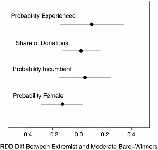
FIGURE 9. Examining the Characteristics of Moderate and Extremist Bare-Winners
The second point estimate in Figure 9 shows, in the same vein, that extremist nominees do not receive fewer primary contributions than do more moderate nominees—another indication that the two types of nominees do not differ in their underlying quality.Footnote 34 The third point estimate tests the hypothesis that extremist bare-winners might be less likely to be incumbents, another form of valence advantage. Paralleling the candidate quality and contribution estimates, we see in the figure that extremist bare-winners are, if anything, more likely to be incumbents, but the effect is small (4.7 percentage points) and we cannot reject the null of no difference.
Possible Demographic Differences of Extremists and Moderates
The final point estimate shows that extremist bare-winners appear roughly 13 percentage points less likely to be female than moderate bare-winners.Footnote 35 While interesting, this difference is unlikely to drive the effect. Evidence on the gender bias of U.S. House elections is mixed, but what evidence there is suggests that any bias would hurt female candidates rather than help them.Footnote 36 This would benefit the extremist bare-winners since they are less likely to be women. That being said, this difference may prove worthy of further investigation in future research. It is likely, based on this test, that extremist bare-winners differ from moderate bare-winners across other salient demographic dimensions as well.
Interest Groups Prefer Moderates
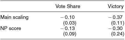
Another possible mechanism—separate from those that depend on particular characteristics of the two types of candidates—is that strategic interest groups and other political actors might support the campaigns of more moderate candidates more than those of extremists in the general election. We know, for example, that interest groups are more moderate than voters on average (Bonica Reference Bonica2013). In the first column of Table 4, I re-estimate the RDD with the share of nonindividual contributions the nominee receives from PACs in the general election as the outcome variable. The nomination of the extremist appears to cause a large decrease—approximately a 30 percentage-point decrease—in the share of contributions coming from PACs.Footnote 37 The results suggest that PACs may play a role in encouraging the penalty to extremists. In addition, we might suspect that the PAC effect is also a proxy for the behavior of other political elites in the district who may likewise withdraw support from extremist nominees.
TABLE 4. Testing Mechanisms, U.S. House 1980–2010
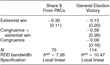
Notes: The first column shows that extremist nominees receive fewer contributions from PACs in the general election. In the second column, we see that the penalty to extremist candidates is larger in districts with greater media congruence and thus more information about the nominee. Robust standard errors in parentheses. Optimal bandwidth from Imbens-Kalyanaraman implemented using rdob in Stata, estimated using local linear OLS.
The Penalty to Extremists Grows With Voter Information
Finally, general-election voters may react directly to the ideological positions of candidates, preferring more moderate positions to more extreme ones (Ansolabehere, Snyder, and Stewart Reference Ansolabehere, Snyder and Stewart, III2001; Burden Reference Burden2004; Canes-Wrone, Brady, and Cogan Reference Canes-Wrone, Brady and Cogan2002; Erikson and Wright Reference Erikson, Wright, Brady, Cogan and Fiorina2000; Tomz and Van Houweling Reference Tomz and Van Houweling2008). This is a likely part of the explanation. Though it is hard to test this mechanism perfectly, we can examine variation in voters’ information about the candidates. Plausibly, voters have less opportunity to react to candidates’ positions when they have little information about the candidates. To test this, I use data on the degree of media coverage the district receives about its own representatives. Specifically, Snyder and Stromberg (Reference Snyder2010) show that the congruence between a district and newspaper markets that provide local political news plays an important role in informing voters about their candidates and elected politicians. Snyder and Stromberg (Reference Snyder2010) show that voters in districts where this congruence is higher—districts where more newspaper information about local politics is available—are more able to identify, describe, and rate their representatives.
I rescale the congruence measure from Snyder and Stromberg (Reference Snyder2010) to run from 0, in the least congruent district in my sample, to 1 in the most congruent, and I interact it with the treatment. The second column of Table 4 presents the results. The penalty to extremists is smaller when information is more scarce and much larger in more congruent districts. Though we cannot reject the null that the effect is the same in the least and most congruent districts, the substantive difference in the effect is extremely large. The penalty to nominating the extremist is estimated to be three times as large in the most congruent district as in the least congruent district.
Identifying the precise channels through which the nomination of the extremist candidate has such pronounced effects is beyond the scope of this study, but investigations into the mechanisms proposed in this section—as well as others—may prove fruitful for future research.Footnote 38 The evidence presented in this section suggests that information about candidates as well as the beliefs and reactions of interest groups help drive the penalty to extremists while, perhaps surprisingly, observable valence differences between extremists and more moderate candidates do not. Because extremists and more moderate candidates in the sample do not differ on observable valences, candidate positions are likely to play a major role in the penalty extremists face in the general election.
CONCLUSION
What happens when extremists win primaries? Recent election cycles, in which an unusual number of especially extreme candidates seem to have won nomination, have left many asking this question. It is difficult to answer, however, because the places that nominate extremists differ systematically from the places that nominate more moderate candidates. The present study addresses this problem by employing a regression discontinuity design in primary elections, which ensures that the places with a moderate or extreme nominee are otherwise comparable in expectation. This allows for the direct estimation of causal effects from the nomination of extremists without the need to model the district’s ideology or to place candidates and districts on a joint ideological scale.
Using this technique, I show that general-election voters punish the nomination of extreme candidates from contested primaries, on average. In fact, the average electoral penalty to nominating an extremist is so large that it causes an observable ideological shift in the district’s subsequent roll-call voting in the opposite direction, towards the opponent party’s ideology. Primary voters thus face a clear tradeoff, on average, between supporting a more “electable” candidate or voting based on ideology and risking the loss of the seat to the other party.
This risk is all the greater because the effects of nominating the extremist extend far into the future. Nominating the extremist today, and risking the loss of the seat today, makes the party much less likely to win the seat in all the subsequent elections within the redistricting period, and likely for much longer. The long-term electoral penalty and roll-call reversal caused by nominating the extremist dispel the notion that extremists can achieve their ideological goals even without winning the seat. In both the short and long run, the nomination of the extremist by one party produces a marked electoral and ideological shift towards the ideology of the opposite party.
Recent political discourse laments the tide of polarization sweeping U.S. legislatures, and a common claim is that primary voters are in part responsible for it. In studying how our electoral system selects candidates for office, and in attempting to explain the sources of the high and growing levels of polarization in our legislatures, we must build on the basic fact that general-election voters in the U.S. House are a tremendous force for moderation in filtering the set of potential candidates for office. When extremists win primaries, they find a supremely challenging electorate standing between them and legislative office.
APPENDIX A: ADDITIONAL STATISTICAL RESULTS
Summary Statistics
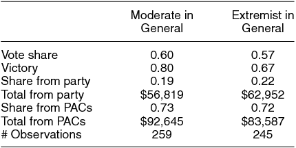
Table A.1 presents summary statistics for the outcome variables of interest, separated out by the “treatment” and “control” cases, i.e., by whether the moderate or extreme candidate wins the primary. We see that moderate nominees tend to have higher general-election vote shares, receive less money from the party, and more money from PACs.Footnote 39 This correlational evidence suggests that the nomination of an extremist over a moderate harms the party, electorally, but it is far from sufficient for making such a conclusion. Districts that nominate extremists are likely to differ markedly from those that nominate moderates. In particular, districts that tend to nominate extremists are likely to have more partisan ideological views, and thus likely to support the nominated extremist in the general election more so than would a moderate, competitive district. The summary statistics are therefore likely to understate the electoral penalty to nominating the extremist. The regression discontinuity design that I employ below confirms this prediction. In fact, the penalty to nominating an extremist is much higher than these statistics suggest.
TABLE A.1. Summary Statistics: Comparing Moderate and Extreme Primary-Winners, U.S. House 1980–2010
External Validity of the Sample
To investigate the external validity of the findings, we can compare the sample to the larger set of all primary elections. The left panel of Figure A.1 plots the distribution of the Democratic district presidential normal vote for all districts and for those entering the analysis. We see that the distributions overlap closely; districts that enter the sample do not appear to differ ideologically from the overall population of primary races.
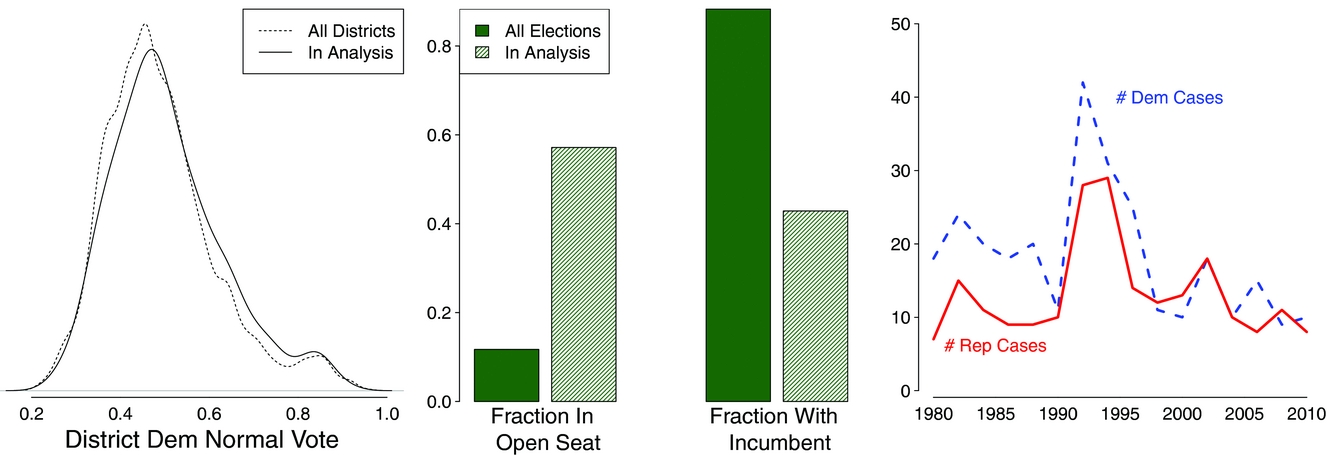
FIGURE A.1. Characteristics of the Sample: U.S. House Primary Elections, 1980–2010
In the middle panel, on the other hand, we see that the primaries entering the sample are much more likely to occur in open-seat races. This makes sense; incumbents have a significant advantage in both primary and general elections (Ansolabehere et al. Reference Ansolabehere, Hansen, Hirano and Snyder2007). As a result, a large number of incumbent-held seats have uncontested or uncompetitive primary elections in both parties and thus do not enter the sample. Finally, the right panel shows that observations in the sample are roughly equally likely to be either Democratic or Republican primaries, and occur consistently over time, with the early 1990s being the most common era represented in the sample.Footnote 40
Open Elections
Figure 3 in the body of the article shows that the effect is large and negative in open-seat races, i.e., those where no incumbent is running in either party’s primary. This is important because it shows that the findings are not driven, on average, by extremist nominees kicking out incumbents. Put another way, the open-seat result shows that the loss of the incumbency advantage is not a mechanism that explains the findings.
To show this result in detail, Table A.2 replicates the main analysis, including the specification reported in Figure 3 (fifth column).
TABLE A.2. RDD Estimates of the Effect of Nominating an Extreme Candidate on General Election Vote Share in Open-Seat Races, U.S. House 1980–2010
Incumbent Presence
Table A.3 presents more tentative results on the effect in races with incumbents. For simplicity, these estimates are presented always using the full data and a cubic polynomial, but findings are similar for other specifications. The first two columns reproduce the full-data specification for the open-seat races from Table A.2 for comparison’s sake.
TABLE A.3. RDD Estimates of the Effect of Nominating an Extreme Candidate on General Election Vote Share, U.S. House 1980–2010
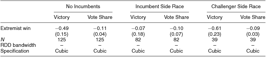
In the second two columns, the effect is estimated only in primaries where an incumbent is present. This is a relatively small number of observations, and many of these races occur in districts safe for the party (third row of Table 1). Because we know the effect is much smaller in safe districts (see Figure 3), it is not surprising that we see the effect attenuate somewhat in these incumbent side races.
The final two columns estimate the effect only for challenger side races in incumbent-held districts, i.e., the primary for the party that does not currently hold the seat. Here the effect is much larger—likely because these primaries tend to occur in more competitive districts (second row of Table 1).
Difference in Effect Across Parties
Table A.4 tests for whether the electoral effects differ across the two parties. To do so, I interact the treatment indicator with an indicator for the primary being a Democratic primary. As the table shows, the effect appears to be smaller (less negative) for Democrats. That is to say, Republican extremist nominees appear to receive a larger electoral penalty in the general election than do Democrats. This does not appear to be driven by differences in how extreme the “extremists” of each party are relative to the their moderate opponents; the average distance between the candidates in the contested primaries is no different across the two parties (difference in means = .009, t = 0.82).
TABLE A.4. RDD Estimates of the Effect of Nominating an Extreme Candidate on General Election Vote Share Across Parties, U.S. House 1980–2010
Validating the RDD Assumption
Like a randomized experiment, the quasi-random variation from the RDD produces balance on pretreatment covariates, in expectation, if the identifying assumption of the RDD is met. We can validate this assumption by checking for balance on observed pretreatment covariates, as in Caughey and Sekhon (Reference Caughey and Sekhon2011) and Eggers et al. (Reference Eggers, Fowler, Hainmueller, Hall and SnyderN.d.). To do so, I re-run Equation 1, but with a variety of pretreatment covariates as the outcome variable. These variables are as follows: absolute distance from 50% of the presidential normal vote in the district (the Democratic presidential normal vote for Democratic primaries, and the Republican presidential normal vote for Republican primaries), averaged over the period 1980–2010, to measure the partisanship of the district; the extreme candidate’s share of primary donations; the extreme candidate’s share of primary donations from PACs; the absolute value of the district’s previous incumbent’s DW-NOMINATE score, to measure the ideology of the district; the absolute value of the district’s previous incumbent’s W-NOMINATE score; and the party’s lagged vote share and electoral victory.
There is some concern with using DW-NOMINATE because it is potentially post-treatment. The dynamic nature of DW-NOMINATE means that votes a legislator casts later in her career can affect her DW-NOMINATE scaling for earlier years. Thus the district’s observed DW-NOMINATE pretreatment may actually include post-treatment roll-call voting. To make sure this is not an issue, I replicate this balance test also using W-NOMINATE scores, which are fixed by congress and therefore do not have this issue. To do so, I collected raw roll-call votes from www.voteview.com and scaled them, by congress, using the wnominate package in R.Footnote 41 To adjust for the fact that the resulting W-NOMINATE scores are not comparable across congresses, which will add noise to the balance test (and thus lower the power of the balance test), I include year fixed effects in this final test.Footnote 42
Table A.5 presents the estimates. As can be seen, there is strong evidence for balance. Estimated differences are small in magnitude, and only 1 out of 24 (4%) of the tests reject the null—roughly the 5% that would be predicted by chance under the null hypothesis (if the tests were independent).
TABLE A.5. RDD Balance Tests
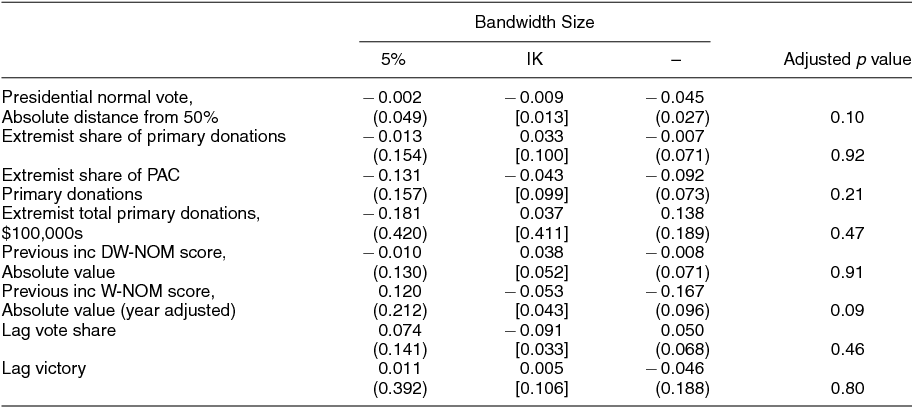
The second rejection is for lagged vote share at the IK bandwidth. As can be seen from the three columns for that test, the results are highly unstable across bandwidths. This is because of the small sample sizes for this test. Because a large number of races occur right after redistricting (see for example the right panel of Figure 2), there are a large number of missing values for lagged electoral outcomes.
To adjust directly for this multiple testing problem, the final column in the table presents adjusted p values for the tests using the cubic specification and the full bandwidth (for brevity’s sake I do not replicate these adjustments for all tests). The adjustment is carried out using a modified version of the “Free Step-Down Resampling” algorithm presented in Anderson (Reference Anderson2008).Footnote 43 This technique adjusts for the covariance among the tests being run and provides exact probabilities rather than bounds. It is therefore less conservative than the Bonferroni test, which is desirable in the present context since we do not want to bias towards not uncovering imbalances if they exist. Not surprisingly, no evidence for imbalance is found using this technique since no test that was not rejected before will be rejected after adjustment.
In addition to these formal tests, Figure A.2 plots the raw data (along with binned averages) for each balance test, excluding only lagged victory because it is a binary variable. Consistent with the table, it is difficult to discern any evidence of sorting.

FIGURE A.2. Graphical Balance Tests
RDD Estimates Across Bandwidths and Specifications
The choice of RDD bandwidth and specification is somewhat arbitrary, so it is important to demonstrate that conclusions are not driven by these choices.
Figures A.3 and A.4 plot the RDD estimate—β1 from Equation 1—across bandwidths for four specifications: the local linear, estimated separately on each side of the discontinuity, and quadratic, cubic, and quartic specifications of the running variable. The plots start from a bandwidth of 3 to ensure a reasonable number of data points enter the estimates. Below 3, the regressions rely on very few observations and, though estimates typically become even more negative, they vary greatly. Since no estimates are presented in the article at bandwidths this small, I omit them from the figures.

FIGURE A.3. RDD Estimate for General-Election Vote Share Across Bandwidths from 3 to 50
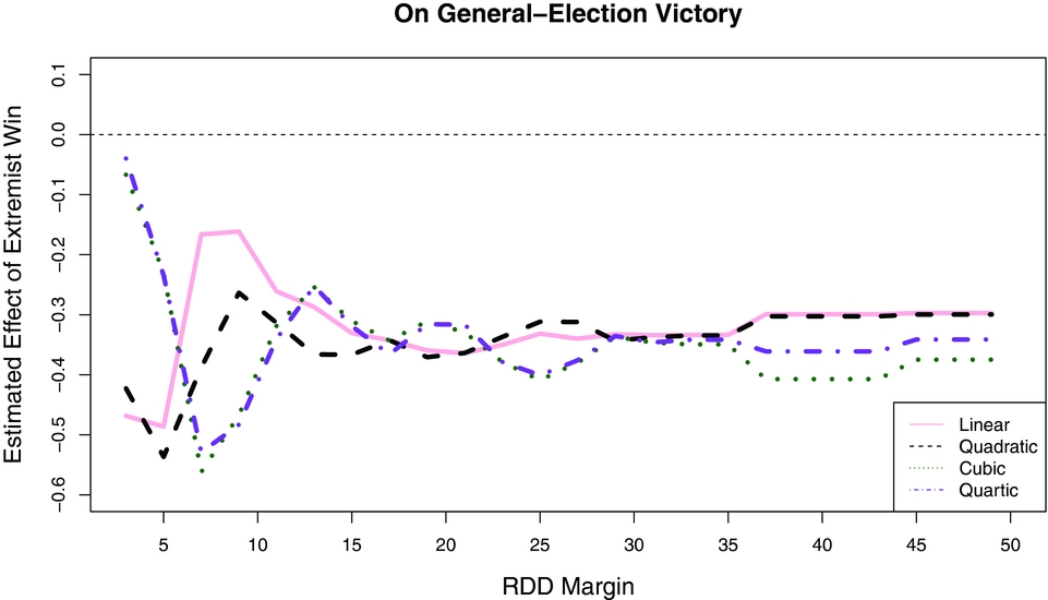
FIGURE A.4. RDD Estimate for General-Election Victory Across Bandwidths from 3 to 50
As the figures show, the conclusions drawn in the article do not vary based on the choice of bandwidth or specification. No matter what specification or bandwidth is used, a large negative effect is found on both vote share and victory, as presented in the article.
To fit as many specifications as possible, these graphs do not include confidence intervals. To give a sense of the noise across bandwidths, Figures A.5 and A.6 plot just the local linear estimate along with 95% confidence intervals. The vast majority of bandwidths support a “statistically significant” finding for the effect both in terms of vote share and victory. There is a small region near 10% where both effects’ confidence intervals cross 0, but it is a small region and is wider than would normally be trusted for a local linear specification (see for example Eggers et al. Reference Eggers, Fowler, Hainmueller, Hall and SnyderN.d.).
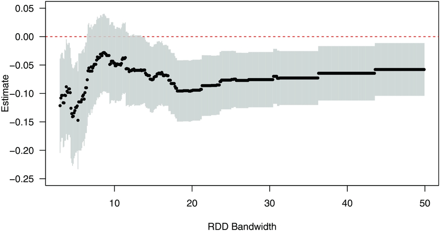
FIGURE A.5. Local Linear RDD Estimate for General-Election Vote Share Across Bandwidths from 3 to 50
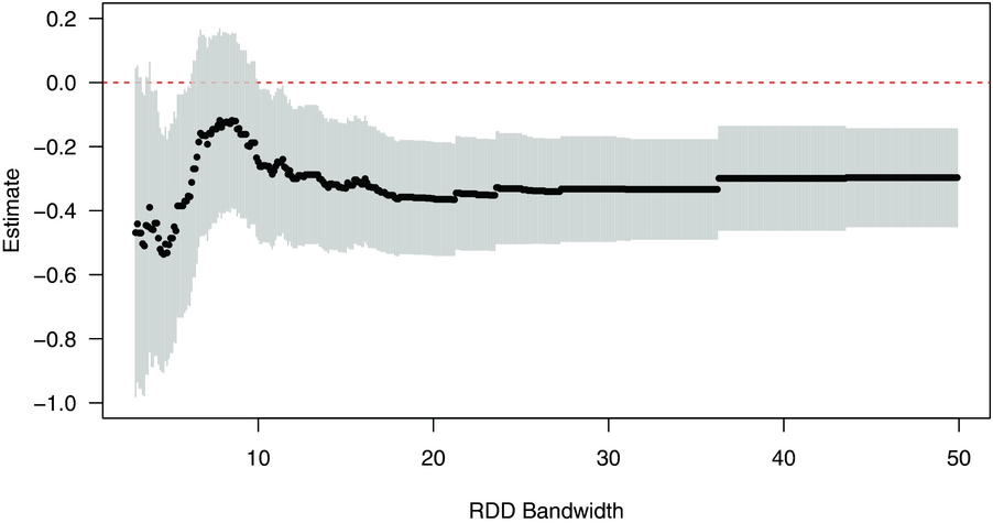
FIGURE A.6. Local Linear RDD Estimate for General-Election Victory Across Bandwidths from 3 to 50
Finally, Figure A.7 plots the same local linear graph for the estimate on candidate quality reported in Figure 9. Again, the vast majority of bandwidths support the conclusion in the article that bare-winner extremists are no more or less likely to hold previous office-holder experience. There is a small region at very small bandwidths where the effect is quite negative—however, the standard errors are very large and the sample sizes are extremely small in this region.
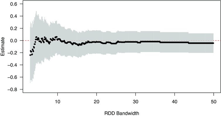
FIGURE A.7. Local Linear RDD Estimate for Nominee Previous Office-Holder Experience Across Bandwidths from 3 to 50
Treatment Intensity
A main complication to the empirical analysis presented in the article is that the binary indicator for “treatment” stands in for a variety of treatment intensities or doses. In some districts that are “treated” with an extremist, the extremist may be relatively moderate, while in other cases she may be quite extreme. To explore this variation in the article, I employ an arbitrarily selected cutoff (the median distance), and I explore how the effect changes as I move this cutoff. To ensure that this cutoff does not drive the results, Table A.6 reports the estimates using no cutoff and instead controls for the distance between the two candidates as well as the interaction of this distance and the treatment.
TABLE A.6. RDD Estimates of the Effect of Nominating an Extreme Candidate on General Election Vote Share, U.S. House 1980–2010
To make the estimates interpretable, I first re-scale the ideological distance variable to run from 0, in the race where the distance between the moderate and the extremist is the smallest, to 1, in the race where this distance is largest. The coefficient on “Extremist Win” in this table thus reflects the estimated causal effect of nominating the “extremist” in a race where the distance between the moderate and the extremist is at the minimum level observed in the whole sample. The coefficient on the interaction reflects the estimated effect in a race where the distance between them is at the maximum level observed in the sample.
The results are consistent with those in the body of the article.
Looking at the first row, we see that the effects appear to be negative (although insignificant) even at the minimal distance. These point estimates are somewhat hard to trust, though, because we know that there is some degree of noise in the underlying scalings of candidates. For candidates already close together, ideologically, we are therefore likely to misclassify some as “extremists” who are actually “moderates” and vice versa. This measurement error in the explanatory variable biases point estimates toward zero.
For vote share, the estimated effect for a race with the maximal distance ranges from − 0.09 (0.01 + − 0.10 = − 0.09 in the IK specification) to − 0.18 (local linear specification). For electoral victory, these effects range from − 0.53 (cubic specification) to − 0.82 (local linear).
The table also reports the p values testing the hypothesis that Extremist Win + Extremist Win · Distance = 0. We can strongly reject the null that the effect is zero for the electoral victory estimates, and we can likewise reject for the vote share estimates with the local linear specification. We cannot reject the null for the cubic and IK specifications here, but the point estimates continue to be substantively large—on the same order as those presented in the article, though the comparison is somewhat difficult due to the differing estimation strategies.
Replicating Results With Alternate Scalings
To ensure that the results are not driven by any issues with the contribution-based scaling, I replicate the main regressions on vote share and electoral victory using a separate measure of candidate ideology that does not rely on donations in any way. To do so I take advantage of competitive primary races where the top two candidates are both state legislators who have compiled an ideological record from the roll-call votes they cast in state legislatures.
Specifically, I focus on primary races where the top two candidates are state legislators who possess NP Scores (Shor and McCarty Reference Shor and McCarty2011). As before, I calculate the absolute distance between the top two candidates in terms of their NP score, and I estimate the RD only using races where this distance is at or above the median distance across all races.
Table A.7 shows the estimates for the party’s vote share and probability of victory. For comparison, the first row reproduces the findings from the article. The second row shows the corresponding estimates identifying moderates and extremists using NP scores instead of contributions. Because there are relatively few such races, the resulting estimates are noisier, but the point estimates are remarkably close to those in the article that rely on the contribution-based estimates.
TABLE A.7. Replicating Results With State Legislator NP Scores
APPENDIX B: SCALING CANDIDATES BASED ON DONATIONS
Below I reproduce the technical details from Hall and Snyder (Reference Hall and Snyder2013). Readers should consult that article for further details and validation exercises.
Let Contribution ij be the contribution (in dollars) that candidate i receives from donor j. We use all donors—both individuals and interest groups—in the procedure.Footnote 44 Consider all incumbents. Let Nominate i be incumbent i’s ideological position, as estimated from i’s roll call voting record using DW-Nominate. Let
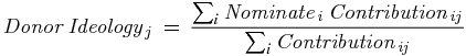 \begin{equation}
\mathit {Donor \, Ideology_{\,j}} \,=\, \frac{\sum _i \mathit {Nominate_{\,i} \, Contribution_{\,ij}}}{\sum _i \mathit {Contribution_{\,ij}}}
\end{equation}
\begin{equation}
\mathit {Donor \, Ideology_{\,j}} \,=\, \frac{\sum _i \mathit {Nominate_{\,i} \, Contribution_{\,ij}}}{\sum _i \mathit {Contribution_{\,ij}}}
\end{equation}
be the average contribution-weighted ideology of the incumbents to which donor j contributes. This gives an estimate of the “revealed ideological preference” of donor j. A possible problem with this definition is that we allow donor contributions to an incumbent candidate to affect that candidate’s own scaling (because that candidate is included in the estimate of the donor’s ideology). To avoid this feedback loop, we produce a separate donor scaling for each candidate i and donor j, where we leave out candidate i in the estimation of donor j’s revealed ideological preference. We define this more nuanced measure as
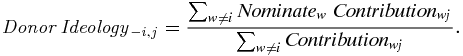 \begin{equation}
\mathit {Donor \, Ideology_{\,-i,j}} = \frac{\sum _{w\ne i} Nominate_w \;Contribution_{wj}}{\sum _{w \ne i} Contribution_{wj}}.
\end{equation}
\begin{equation}
\mathit {Donor \, Ideology_{\,-i,j}} = \frac{\sum _{w\ne i} Nominate_w \;Contribution_{wj}}{\sum _{w \ne i} Contribution_{wj}}.
\end{equation}
Finally, for each candidate k, let
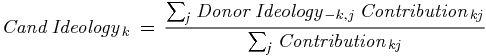 \begin{equation}
\mathit {Cand \, Ideology_{\,k}} \,=\, \frac{\sum _j \mathit {Donor \, Ideology_{\,-k,j} \, Contribution_{\,kj}}}{\sum _j \mathit {Contribution_{\,kj}}}
\end{equation}
\begin{equation}
\mathit {Cand \, Ideology_{\,k}} \,=\, \frac{\sum _j \mathit {Donor \, Ideology_{\,-k,j} \, Contribution_{\,kj}}}{\sum _j \mathit {Contribution_{\,kj}}}
\end{equation}
be the contribution-weighted average $\mathit {Donor \, Ideology}$
of all donors that contribute to k. This serves as our estimate of the ideological position of candidate k. To make the measure more reliable, we exclude donors who make fewer than 20 donations to distinct candidates in our data, and we also exclude candidates who receiver fewer than 20 donations from distinct donors.Footnote
45
Later we present results to show that our analysis is not dependent on the choice of threshold. Also in contrast to other scaling methods, we only use donations made during the primary-election cycle when scaling candidates, in order to avoid concerns that strategic interest groups target electable candidates in the general election (and thus make those candidates appear more moderate in the scaling).
$\mathit {Donor \, Ideology}$
of all donors that contribute to k. This serves as our estimate of the ideological position of candidate k. To make the measure more reliable, we exclude donors who make fewer than 20 donations to distinct candidates in our data, and we also exclude candidates who receiver fewer than 20 donations from distinct donors.Footnote
45
Later we present results to show that our analysis is not dependent on the choice of threshold. Also in contrast to other scaling methods, we only use donations made during the primary-election cycle when scaling candidates, in order to avoid concerns that strategic interest groups target electable candidates in the general election (and thus make those candidates appear more moderate in the scaling).
We create two versions of these scalings. In the first, we use general-election and primary-election donations to all candidates to scale donors (and then use only primary donations from these groups to scale candidates). There is some concern that this method confounds “moderation” with electoral desirability, if some donors are strategic in whom they contribute to. For example, interest groups might donate to incumbents because incumbents are likely to win reelection. This donation behavior would make these interest groups appear moderate (because they would be donating to people from both parties), and in turn make the incumbents they donate to appear moderate, thus creating an artificial link between candidate moderation and electoral success. Even though we never use incumbents in our main analyses, these same interest groups might donate to other candidates in open-seat races, contaminating their estimated ideologies. We therefore construct a second version in which we do not use any donations to incumbents when scaling donors, and in which we do not use any donations to candidates after they become incumbents when scaling candidates.Footnote 46 Throughout the article, we present all of our results using both versions, to stress that they lead to the same conclusions.
To recap, here are the general steps taken to produce our scalings. For each candidate i, we do the following:
-
1. Estimate donor ideology for candidate i according to Equation 3 based either on Nominate scores of incumbent recipients or based on party affiliation of all recipients, using either (a) primary and general-election donations to all candidates excluding candidate i or, (b) primary and general-election donations to nonincumbent candidates, excluding candidate i.
-
2. Impute ideology for candidate i according to Equation 4, based either on the imputed Nominate or party affiliation scores of donors, using either (a) primary-election donations to all candidates or, (b) using only primary-election donations to nonincumbent candidates.Footnote 47