II. RELATED WORKS

Although the problem of multiple compression detection is relatively new in the multimedia forensics, several works on double compression detection have been presented in the literature. Some of the proposed solutions analyze the statistics of DCT coefficients [Reference Pevny and Fridrich7]. The second compression implies a re-quantization of DCT coefficients that are re-distributed among the bins of the second quantizer following a different statistics with respect to single compressed images. In [Reference Lin, He, Tang and Tang13], Lin et al. observe that double quantization introduces periodicities in coefficient statistics, which can be exploited to reveal double compression and the set of parameters used. Similarly, the work in [Reference Pevny and Fridrich7] detects the peculiar modifications on coefficients statistics brought by double quantization using an support vector machine (SVM) classifier. The approach in [Reference Fu, Shi and Su14] generalizes the Benford's law for the DCT coefficients and checks its consistency on the analyzed image (more details will be provided in Section III). Other strategies rely on the assumption that quantization is an idempotent operation, i.e., requantizing DCT coefficients with the same quantizer leads to reconstructed values highly-correlated with its input [Reference Xian-Zhe, Shao-Zhang and Jian-Chen15]. In [Reference Barni, Costanzo and Sabatini16], the authors detect double compression by studying coding artifacts. In [Reference Qu, Luo and Huang17] a convolutive mixing model is presented in order to deal with the problem of shifting the image between the first and the second compression. Other methods rely on modelling the statistics of natural images. These include the approaches based on the analysis of the distribution of the first significant digits, which can be modeled according to Benford's law [Reference Li, Shi and Huang18].

Many of these solutions are employed to detect tampering [Reference Lukás and Fridrich4], steganalysis [Reference Pevny and Fridrich7], or forgery localization [Reference Bianchi, Rosa and Piva19]. The main idea lying at the base of these approaches is that distinguishing double compressed regions from single compressed regions permit identifying which parts have been modified and which are original.

In the following, we will show how it is possible to extend the approaches based on Benford's law to the detection of multiple compression on images.

III. MULTIPLE COMPRESSIONS AND COEFFICIENTS STATISTICS

A) The JPEG compression standard

The JPEG image compression standard defines a block-based transform coder (see Fig. 1), which partitions the input image into 8 × 8 pixel blocks X and computes the DCT of each block. Transform coefficients Y are quantized into integer-valued quantization levels Y _Δ1 ¹

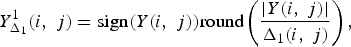(1) $$Y_{\Delta_1}^1\lpar i \comma \; j\rpar = \hbox{sign}\lpar Y\lpar i\comma \; j\rpar \rpar \hbox{round} \left(\displaystyle{{\vert Y\lpar i\comma \; j\rpar \vert }\over{\Delta_1\lpar i\comma \; j\rpar }} \right)\comma \;$$

where the indexes (i, j), i, j = 0, …, 7, denote the position of the elements in the 8 × 8 block. The values Y _Δ1 ¹ (i, j) are converted into a binary stream by an entropy coder following a zig-zag scan that orders coefficients according to increasing spatial frequencies. The coded block can be reconstructed by applying an inverse DCT transform on the rescaled coefficients Y _r ¹(i, j) = Y _Δ1 ¹ (i, j) · Δ₁ (i, j). Note that the quantization step Δ₁ (i, j) changes according to the index (i, j) of the DCT coefficient and is usually defined by means of a quantization matrix. In the Independent JPEG Group (IJG) implementation, the quantization matrix is selected by adjusting a quality factor (QF), which varies in the range [0, 100]. The higher QF, the higher the quality of the constructed image.

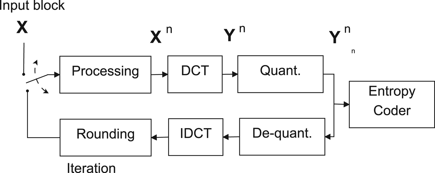
Fig. 1. Bock diagram for multiple JPEG compression.

When the image is encoded a second time, the resulting quantization levels are

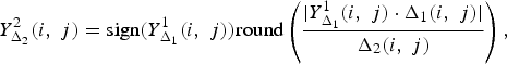(2) $$Y_{\Delta_2}^2 \lpar i\comma \; j\rpar = \hbox{sign}\lpar Y_{\Delta_1}^1 \lpar i\comma \; j\rpar \rpar \hbox{round}\left(\displaystyle{{\vert Y_{\Delta_1}^1\lpar i\comma \; j\rpar \cdot \Delta_1\lpar i\comma \; j\rpar \vert }\over{\Delta_2\lpar i\comma \; j\rpar }} \right)\comma \;$$

where Δ₂(i, j) are the quantization steps of the second compression stage.Footnote ¹ It is possible to iterate the compression process N times leading to the quantization levels Y _{Δ N} ^N (i, j).

B) The FD law

Many fraud detection algorithms departs from the assumption that the analyzed data are well modeled by pre-defined stochastic models that present peculiar characteristics. A similar assumption is adopted by many approaches aiming at detecting double JPEG compression. More precisely, some of the proposed works rely on detecting the violation of the so-called Benford's law (also known as FD law or significant digit law) [Reference Wang, Cha, Cho and Kuo20]. Many fraud detection algorithms departs from the assumption that the analyzed data are well modeled by pre-defined stochastic models that present peculiar characteristics. One of these is the FD rule, which proves to be satisfied for many distributions. The most significant digit or FD for a strictly-positive integer Y (in base-10 notation) can be computed as

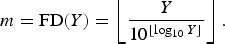(3) $$m = {\rm FD}\lpar Y\rpar = \left\lfloor \displaystyle{{Y}\over{10^{\lfloor \log_{10} Y\rfloor}}} \right\rfloor.$$

It is possible to state that Benford's law [Reference Benford9] is satisfied whenever the pmf of m can be well approximated by the equation

(4) $$p\lpar m\rpar = N \log_{10}\left(1 + \displaystyle{{1}\over{m}}\right)\quad \quad \quad \quad{\rm or }$$

(5) $$p\lpar m\rpar = N \log_{10}\left(1 + \displaystyle{{1}\over{\beta + m^\alpha }}\right)\quad \hbox{\lpar generalized \rpar \comma}$$

where N is a normalizing factor and α,β are the parameters characterizing the model. This property can be verified for many real-life sources of data and can be effectively used to detect alterations on the analyzed data. Indeed, whenever some kind of modification has been performed on a dataset that originally satisfies Benford's law, the resulting distribution no longer satisfies this property. This fact has been widely employed in fraud detection in different fields (elections [Reference Battersby21, Reference Deckert, Myagkov and Ordeshook22], budget [Reference Nigrini23, Reference Müller24], etc.), as well as in detecting double compression in JPEG images [Reference Fu, Shi and Su14].

C) Statistics of coefficients and FDs after multiple compressions

The single and double compressions of an image leave different peculiar traces on the statistics of coefficients and their FDs. Most of the double compression detectors use these traces to decide whether an image has been compressed once or not. For the sake of conciseness, we will refer to the absolute DCT quantized coefficients after the Nth compression as y _N  = |Y _{Δ N} ^N | (position indexes (i, j) have been omitted for the sake of clarity) and their corresponding FDs m _N  = FD(y _N ).

When multiple compressions are applied, each compression stage modifies the statistics of coefficients and their corresponding FDs leaving denotative elements.

Fig. 2 reports the pmf of FDs for DCT coefficients at different coding stages for the image house of the Kodak dataset. The adopted quantization factors are QF ₄ = 85, QF ₃ = 76, QF ₂ = 80, and QF ₁ = 85. The same figure also reports the discrete fourier transform (DFT) of the difference (parameter χ) between the actual pmf of FDs and its interpolated version following Benford's law, i.e., χ(m _N ) = P[m _N  = k] − p(m _N ). Figures 2(e)–2(h) show that the most significant oscillations take place at peculiar normalized frequencies of DFT coefficients. For single compressed images, oscillations are quite limited (DFT coefficients are lower than 0.17). In case an image is double compressed (Fig. 2(f)), part of the energy of χ is concentrated around F = 0.2 (where F is the normalized frequency for DFT transform). Note that in this case the maximum value of DFT coefficients is higher with respect to the case of images compressed once. For images compressed three times, the DFT plots show that two oscillating modes appear at F ≃ 0.18 and F ~ 0.28 (Fig. 2(g)), while four compressions lead to stronger oscillations dominated by the component at F = 0.34 (FFT results highly peaked in Fig. 2(h)).

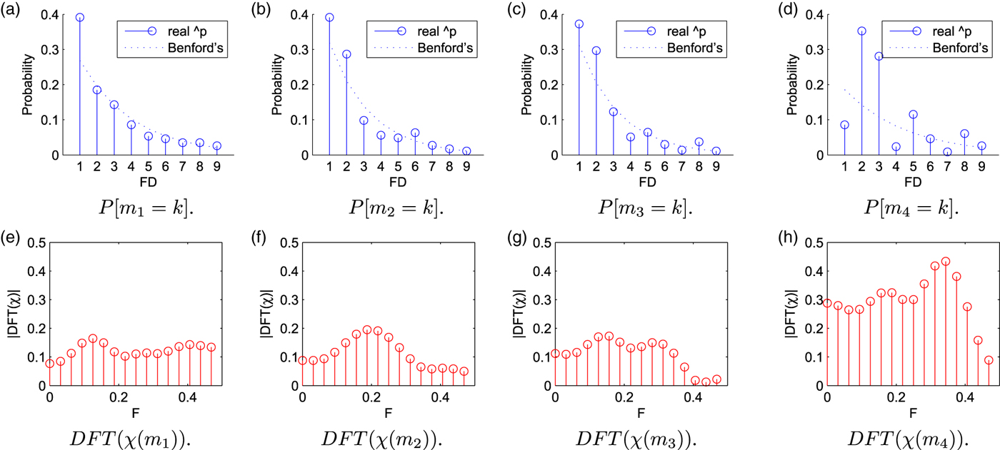
Fig. 2. Probability mass functions of FDs and frequency spectra of their differences χ(y _N ) with respect to a Benford's model at different coding stages. The parameter F denotes the normalized frequency for DFT coefficients of χ. The graphs are related to coefficient at position (1, 0) for image house. (a) P[m ₁ = k]. (b) P[m ₂ = k]. (c) P[m ₃ = k]. (d) P[m ₄ = k]. (e) DFT(χ(m ₁)). (f) DFT(χ(m ₂)). (g) DFT(χ(m ₃)). (h) DFT(χ(m ₄)).

Ad-hoc solutions need to be designed in order to reveal the presence of these oscillations in the statistics of the FD for transform coefficients. In fact, previous solutions targeted simple double compression detection, i.e., were aimed at verifying the regularity of the actual FD statistics $\hat{p} \lpar m\rpar$ . Multiple compression detection requires characterizing the characteristics of deviations from Benford's law. As a result, double compression detectors fail in discriminating the number of coding stages and the corresponding coding parameters.

It is possible to overcome this problem by combining a set of classifiers, as it will be described in the next section.

IV. THE PROPOSED DETECTION ALGORITHM

The estimation of the number of coding stages N requires to select a set of robust features that present a strong correlation with the traces left by quantization. From this selection, it is possible to design a set of classifiers associated to each compression stage. Their outputs can be combined estimating the number of compressions operated on the image under analysis.

To this purpose, we generated an exhaustive dataset of compressed images, where the number of compressions operated on each picture can vary from 1 to 4. The adopted JPEG codec is the one implemented in the MATLAB software. The quality factor QF _i of the ith compression stage is selected randomly within an interval of possible values [QF _N  − dQF, QF _N  + dQF], where QF _N is the QF of the last compression stage and dQF is the halved width of the interval. This limit was imposed in order to constrain the quality degradation in the final image since significant variations in the QF values across the different compression stages introduce evident unnatural artifacts on the reconstructed pictures.

Moreover, we also imposed that the difference between the chosen QFs of two consecutive compression stages must be higher than a threshold T _QF , i.e. |QF _i  − QF _i+1| > T _QF . This constraint was introduced in order to make the quantization steps for all the considered DCT coefficients change from one compression stage to the following.

In the literature, the set and the number of analyzed DCT coefficients employed by different double compression detectors can change. In [Reference Li, Shi and Huang18], 20 spatial frequencies were considered, while in the approach [Reference Pevny and Fridrich7] only 9 frequencies are considered. Note that most of these frequencies lies at low frequencies since DCT coefficients at low frequencies proves to be more regular and changes less significantly according to the characteristics of the image with respect to those located at high frequencies. Moreover, high-frequency coefficients are often quantized to zero, and therefore, their statistics can only be computed from a limited amount of data. In this approach, we adopted the set of coefficients in [Reference Pevny and Fridrich7]. Then, we set T _QF  = 5 since, according to the values of the quantization matrix of the JPEG codec implemented by MATLAB, it ensures that none of the DCT coefficients at compression stage i is quantized with Δ _i  = Δ _i−1.

Three different datasets were generated. In a first dataset D ₀, the compression grids of images are aligned, i.e., no transformation was operated on the image between one compression stage and the following. In a second dataset D ₁, images were rescaled at a random compression stage, where the rescaling factor was randomly-chosen in the interval [0.9, 1.1]. In the third dataset D ₂, images are rotated of a random angle included in the interval [−5, 5] at a randomly-selected compression stage. In this way, datasets D ₁ and D ₂ introduce the possibility that the compression grids could not be aligned (since they include both transformed and unaltered images).

In the following, we will describe the feature extraction process and the training of the classifiers for the dataset D ₀. The same operations are applied on the datasets D ₁ and D ₂ as well.

A) Feature selection

Given a JPEG image I ⁿ which has been compressed n times, most of the approaches existing in the literature extract the quantized DCT coefficients of the luma component and compute a set of features from their statistics. Features may include the simple FD statistics for the DCT coefficients at low frequencies [Reference Li, Shi and Huang18] or the relative difference between the actual pmf and the Benford's equation, i.e. $\chi\lpar m\rpar = \lpar p\lpar m\rpar - \hat{p}\lpar m\rpar \rpar /\hat{p}\lpar m\rpar $ [Reference Fu, Shi and Su14].

In our approach, we adopted the first possibility computing the pmfs of FDs on the set of nine spatial frequencies reported in [Reference Pevny and Fridrich7]. This would lead to a feature array of 9 × 8 = 72 values,Footnote ² but we aim at reducing this size by properly selecting those features that are extremely sensible to the number of compression stages. More precisely, Fig. 2 shows that the probabilities for some FD values are more sensitive to multiple compression than others, i.e., the deviation from Benford's law equation is more discriminative. From this premise, it is possible to select a subset of l probability values p(k ₁), … , p(k _l ) from the pmf of FD digits (k ₁, …, k ₂ ∈ [1, 9]).

Naming $\hat{p}_{F_{h}\comma m}\lpar k\rpar = P_{F_{h}}\lsqb m == k\rsqb $ the probability that the FD value m for the coefficients located at spatial frequency F _h is equal to k, it is possible to gather the features in a common array

(6) $$\eqalign{{\bf f} &= \lsqb p_{F_1\comma m}\lpar k_1\rpar \cdots p_{F_1\comma m}\lpar k_l\rpar p_{F_2\comma m}\lpar k_1\rpar \cdots p_{F_2\comma m}\lpar k_l\rpar \cdots\cr &\quad \times p_{F_9\comma m}\lpar k_1\rpar \cdots p_{F_9\comma m}\lpar k_l\rpar \rsqb .}$$

Note that features are already limited in the range [0, 1] since they are related to pmf of FD values.

In order to find the optimal set of features, we considered different sets of $\hat{p} \lpar m\rpar$ values changing both the values k ₁, …, k _l and their number l. To this purpose, we randomly selected 1200 images from the UCID dataset [Reference Schaefer and Stich25] which were compressed once and twice with different quantization parameters QF. The quantization parameter of the last coding stage is fixed (since it is known from the coded bit stream), while the QF adopted in the first stage is randomly chosen in the interval [QF − 10, QF − 5] ∪ [QF + 5 , QF + 10]. In this part, 10 different realizations were generated for every image. From these images, we computed the vectors f and used them in training a binary SVM classifier that discriminates single from double compressed images. The remaining 100 images in the UCID dataset were double compressed in a similar manner and used for testing the accuracy of the classifier. In this case, the double compression detector is taken as a simplification of the multiple compression detector for the sake of complexity since training the full multiple compression detector for all the configurations would require a significant time.

Fig. 3(a) reports the average detection using a feature array f with l = 3, where the feature array has been created selecting only a subset (k ₁, k ₂, k ₃) of possible FD values, i.e., f = [p _{F h,m} (k ₁) p _{F h,m} (k ₂) p _{F h,m} (k ₃)] _{F h} . The different results have been obtained considering all the possible combinations for k ₁, k ₂, k ₃. For the sake of clarity, the triplet [k ₁, k ₂, k ₃] is indexed by the value (k ₁ − 1) + (k ₂ − 1) 9 + (k ₃ − 1) 81 (reported on the x-axis). It is possible to see that the triplet [Reference Milani2, Reference Wallace5, Reference Milani, Tagliasacchi and Tubaro6] permits obtaining the highest accuracy. Note also that the length of the feature vector is 27. It is also possible to verify that the obtained accuracy is comparable with that obtained by decomposing the feature array f with l = 8 using a principal component analysis (PCA) and selecting the three most relevant components. Building a new classifier on this feature array obtained from PCA, it is possible to obtain an average accuracy of 92%. Nevertheless, the PCA-based classifier requires computing all the features in advance and then transform the feature array into its principal component representation. The proposed solution requires to compute only three features for each spatial frequency.

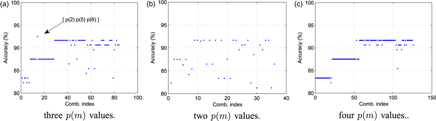
Fig. 3. Accuracy of single versus double compression detector for different feature arrays. (a) three p(m) values, (b) two p(m) values, and (c) four p(m) values.

We also considered the possibility of increasing or reducing the number l of features in f. Additional Figs 3(b) and 3(c) report the average accuracy of the detector when l = 2 (f = [p _{F h ,m} (k ₁) p _{F h ,m} (k ₂)] _{F h} ) and l = 4 (f = [p _{F h ,m} (k ₁) p _{F h ,m} (k ₂) p _{F h ,m} (k ₃) p _{F h ,m} (k ₄)] _{F h} ), respectively. Note that this would lead to feature arrays of 18 and 36 elements. The adopted set k ₁, …, k _l of probability values is changed as for Fig. 3(a) and each configuration is indexed by the values (k ₁ − 1) + (k ₂ − 1) 9 for l = 2 and (k ₁ − 1) + (k ₂ − 1) 9 + (k ₃ − 1) 81 + (k ₄ − 1) * 729 for l = 4. Indexes are reported on the x axes.

It is evident that using 3 values proves to be the best solution since the maximum average accuracy is higher than using 2 or 4 probability values. In the first case, the feature space does not allow an effective clustering, whereas in the second the additional feature does not improve the classification accuracy.

As a results, each image is represented with a feature vector f of 27 elements (i.e., approximately six times smaller than in [Reference Li, Shi and Huang18]).

The following section will show how the final classifiers are designed starting from the feature vectors f.

B) Design of the classifiers

Given the dataset D ₀, we computed the features f with k ₁ = 2, k ₂ = 5, and k ₃ = 6 for every image. The dataset was divided into two subsets D ₀ ^t , D ₀ ^v to train (D ₀ ^t ) and validate (D ₀ ^v ) the detector, respectively.

Assuming that the quality factor QF of the last compression stage is known (from the available bitstream), we built a set of N _T binary SVM classifiers, ${\cal S}_{QF\comma k} \lpar k = 1\comma \; \ldots\comma \; N_{T}\rpar $ , where each classifier ${\cal S}_{QF\comma k}$ is able to detect whether the input image has been coded k-times or not.

In designing ${\cal S}_{QF\comma k}$ , we adopted the exponential kernel

(7) $$K \lpar {\bf f}_i\comma \; {\bf f}_j\rpar = \exp -\gamma_k \left(\Vert {\bf f}_i - {\bf f}_j \Vert _2^{\gamma_k} + 1 \right).$$

The parameter γ _k and the kernel type were optimized in the training phase computing the structure that gives the optimal performance. In this process, we adopted a cross-validation optimization based on the RANSAC algorithm. The training is carried out looking for the best γ _k value that maximizes the recall value for each class, i.e., maximizing the probability of correct classification for each subset of training images coded N times. Each classifier also outputs a confidence value w _k that reports the distance from the discriminating hyperplane and permits evaluating the reliability of the classification.

Similarly, second set of classifiers, named O _{QF, k−t} , is generated which discriminate whether an images has been coded either k or t times. Naming s _k the output of the classifier S _{QF, k} and o _k−t the output of O _{QF, k−t} , the outcomes of the different classifiers are combined together in order to make the estimation more robust.

Outputs are combined in the feature vector

(8) $${\bf f}_{cl} = \lsqb s_1 s_2 s_3 s_4 o_{1-2} o_{1-3} o_{1-4} o_{2-3} o_{2-4} o_{3-4}\rsqb \comma \;$$

which has to be related to the number of compression. It is possible to relate f _cl to the unknown number of compressions N that were applied to the analyzed image by training an regressor processing f _cl . Figure 4 reports the whole detection scheme.

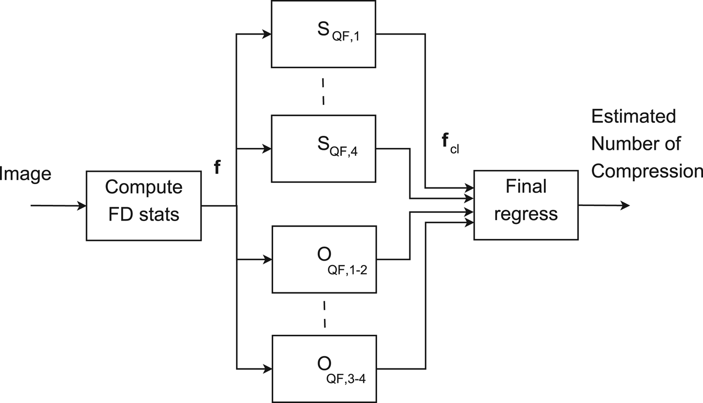
Fig. 4. Block diagram of the proposed detector.

Performance was tested on the validation dataset D ₀ ^v and results are reported in the following section. A similar procedure was applied on the datasets D ₁ and D ₂.

V. EXPERIMENTAL RESULTS

As it was reported in the previous section, the detector was designed from a training database of images compressed up to four times. In order to generate the training database, we randomly selected the 100 images from the UCID dataset [Reference Schaefer and Stich25]. Each image was coded up to four times with a random sequence of quality factors QF _i for each compression stage. The quantization factor QF _i at stage i is randomly chosen in the interval [QF _i+1 ^l  − 12, QF _i+1 ^l  − 6] ∪ [QF _i+1 ^u  + 6, QF _i+1 ^u  + 12], where QF _i+1 ^l and QF _i+1 ^u are the lower and upper QF limits that ensure that the quantization steps related to QF _i differ with respect to those of QF _i+1.

These images were included in the datasets D ₀ ^t , D ₁ ^t , and D ₂ ^t . A set of 200 images among the remaining pictures of the UCID dataset were compressed in the same ways and included in the datasets D ₀ ^v , D ₁ ^v , and D ₂ ^v .

Since the dataset was extended with respect to the tests in [Reference Milani, Tagliasacchi and Tubaro6], the performance proves to be slightly worse on average despite the approach proves to be effective in many cases. To provide evidence for this, we make available a demo version of the multiple compression detection algorithm for download at [Reference Milani26].

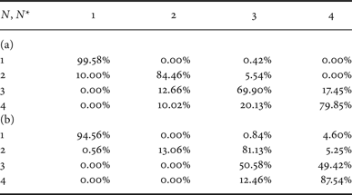
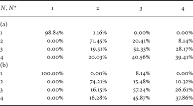
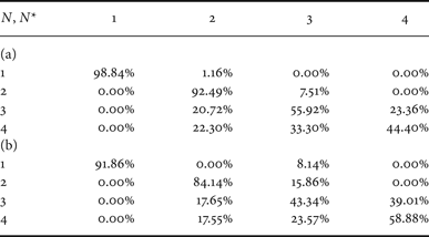
Table 1(a) shows a confusion matrix for dataset D ₀. The real number of compression stages is reported along the rows while the estimated number of compressions is reported along the columns. Each cell (u, v) reports the percentage of images compressed u times that were detected as compressed v times. It is possible to notice that the case of a single compression stage is always correctly identified. In the case an image was compressed 1, 2 or 3 times, the proposed method performs quite well since the probability of correct detection is above 84.8%. The average accuracy is around 83%. We compare the performance with that of a classifier designed adapting the work in [Reference Li, Shi and Huang18] in order to detect the number of compression stages. The confusion matrix, which is shown in Table 1(b), demonstrates that the two methods achieve nearly the same results for N = 1, but the average accuracy of the second solution is lower (~62%) with respect to the proposed solution. In this latter case, a significant performance loss is evident for N = 2. This is due to the difficulty in identifying an adequate set of support vectors, because of the high dimensionality of feature vectors and the increased amount of compression noise introduced. The performance increases for N > 2 since the availability of the full pmf of the FDs permits including those features that present wider oscillations whenever the image is compressed three or four times (e.g., p(2) and p(5) as Figs 2(c) and 2(d) show).

Table 1. Confusion matrix for QF _N  = 75 and dataset D ₀. (a) Proposed method, (b) classifier in [Reference Li, Shi and Huang18] (adapted).

Results for quality factor QF = 80 are reported in Table 2. In this case, the average precision is 88% but the performance of the detector in identifying N = 3 or 4 compressions improves. In this case, the adopted quantization steps are smaller and the amount of compression noise is lower permitting a more accurate detection even after more than two compression stages. Also in this case the approach in [Reference Li, Shi and Huang18] (adapted to detect multiple compressions) presents a lower accuracy (~85%).

Table 2. Confusion matrix for QF _N  = 80 and dataset D ₀. (a) Proposed method, (b) classifier in [Reference Li, Shi and Huang18] (adapted).

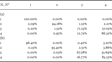
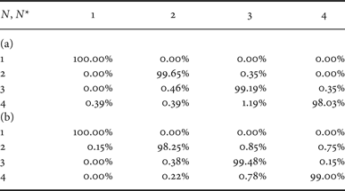
Table 3 reports the confusion matrix when QF _N  = 90. It is possible to notice that the difference between the performances of the two approaches is significantly reduced. This fact is mainly correlated with the percentage of non-null quantized coefficients in each image. At low QF values, many coefficients are quantized to zero, and therefore, the FD probabilities are computed from a reduced amount of coefficients. Since in this case the statistics is diluted, many probability values with l = 8 are not reliable features for the classification. Shrinking the array f to the subset of the most reliable features permits increasing the accuracy of the detection.

Table 3. Confusion matrix for QF _N  = 90 and dataset D ₀. (a) Proposed method, (b) classifier in [Reference Li, Shi and Huang18] (adapted).

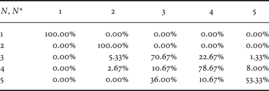
In the end, we also evaluated the possibility of detecting five compression steps for the images adopted to generate dataset D ₀. In this case, confusion matrix for the proposed approach is reported in Table 4. It is possible to notice that, although the average accuracy is decreased to 80%, the capability of detecting N < 5 compression stages is increased. This fact is mainly due to the fact that the detectors are trained with images coded more than four times, and as a consequence, the partitionings of features space operated by the SVM classifiers are more accurate.

Table 4. Confusion matrix with QF _N  = 80 on dataset D ₀ for the detection of five compression stages (proposed algorithm).

It is possible to notice that the accuracy of the method based on [Reference Li, Shi and Huang18] (adapted) increases as the compression quality increases. This fact is mainly correlated with the percentage of non-null quantized coefficients in each image.

At low QF values, many coefficients are quantized to zero, and therefore, many probability values $\hat{p}_{F_{h}\comma m}\lpar k\rpar $ are computed from a reduced set of data and do not provide reliable features for the classification. Shrinking the array f to the subset of the most reliable features permits increasing the accuracy of the detection. It is possible to notice that at high QF values (low distortion) the accuracy of the approach in [Reference Li, Shi and Huang18] get closer to that of the proposed approach.

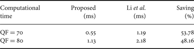
The proposed method is characterized by a lower computational complexity with respect to the approach in [Reference Li, Shi and Huang18], since the size of the feature vector is much smaller.

We also tested the improved accuracy of the proposed classifier in a simple double compression detection (i.e., verifying whether an image has been compressed once or more times). More precisely, tested the SVM classifier proposed in [Reference Li, Shi and Huang18] with respect to the classifier using the features in equation (8), which compose different SVM classifiers using a reduced set of features. Figure 5 reports the receiver operating characteristic (ROC) curves of the two approaches for different QFs. It is possible to see that the proposed detector is much more effective in detecting double compression.

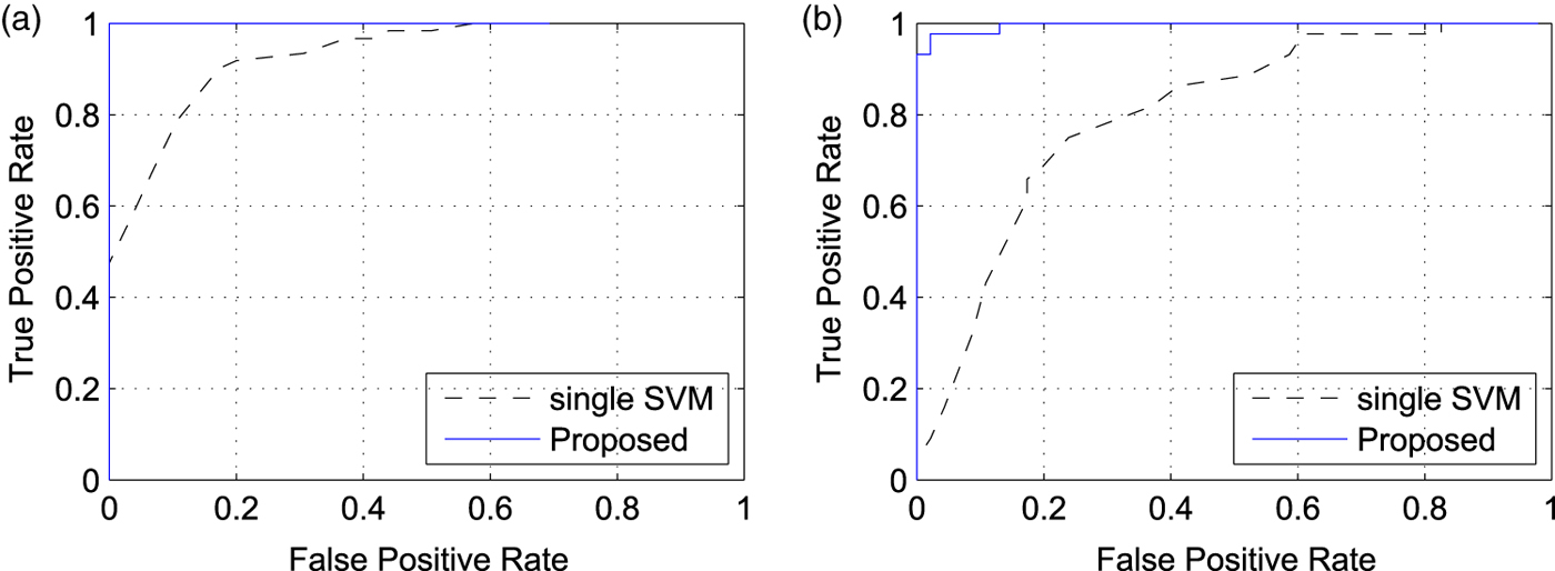
Fig. 5. ROC curves of different double compression detectors for different QFs on dataset D ₀. (a) QF = 70, (b) QF = 80.

Table 5. Computational time for the proposed method and the classifier in [Reference Li, Shi and Huang18] (adapted).

Furthermore, we considered the robustness of the approach changing the range of variation for the QF parameters. More precisely, we changed the width dQF of the interval where QF values are randomly chosen. Figure 6 reports the average accuracy obtained changing the width of the interval as a function of dQF. It is possible to notice that increasing the range of QF values leads to a decrement of the detection performance and of the average peak signal-to-noise ratio (PSNR) value after N coding stages.

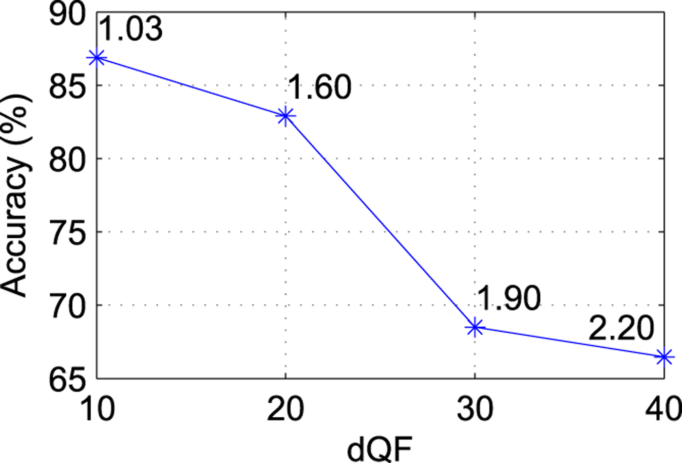
Fig. 6. Accuracy versus dQF for images coded with QF _N  = 70 on dataset D ₀. The graph also reports the average PSNR decrement (dB) for each point.

Finally, we also tested the robustness of the approach in case an image is manipulated between consecutive compression stages. More precisely, we assumed that image manipulation took place at the processing block in Fig. 1, before one of the coding stages.

In the processing chain, we introduced a random manipulation which could consist either in a rescaling or in a rotation. The idea is to disalign the block grid of JPEG compression in order to test the robustness of the detector. The parameter values for each transformation are random as well and can vary in the intervals [.9, 1.1] for the rescaling (the parameter is the pixel width ratio), and [−5, 5] for the rotation angle. These limits are justified by the need of avoiding a significant decrement of the image quality and keeping the size of the transformed image close to that of the original one. These data were collected in the datasets D ₁ and D ₂.

The confusion matrix in Table 6 was obtained from dataset D ₁ and show that the proposed classifier permits obtaining an average accuracy of 65%. Note also that increasing the size of the feature vector f (see Table 6(b)) does not bring significant improvements in terms of performance, made exception for the detection of three compression stages. The approach in [Reference Li, Shi and Huang18] permits obtaining an average accuracy equal to 62% in presence of random rescalings.

Table 6. Confusion matrix for QF _N  = 80 from datasets D ₁. (a) Proposed method, (b) classifier in [Reference Li, Shi and Huang18] (adapted).

As for the dataset D ₂, Table 7 shows that the proposed solution permits obtaining an average accuracy equal to 75%, while the solution derived from [Reference Li, Shi and Huang18] permits having an average accuracy of 69%.

Table 7. Confusion matrix for QF _N  = 80 from datasets D ₂. (a) Proposed method, (b) classifier in [Reference Li, Shi and Huang18] (adapted).