
Introduction
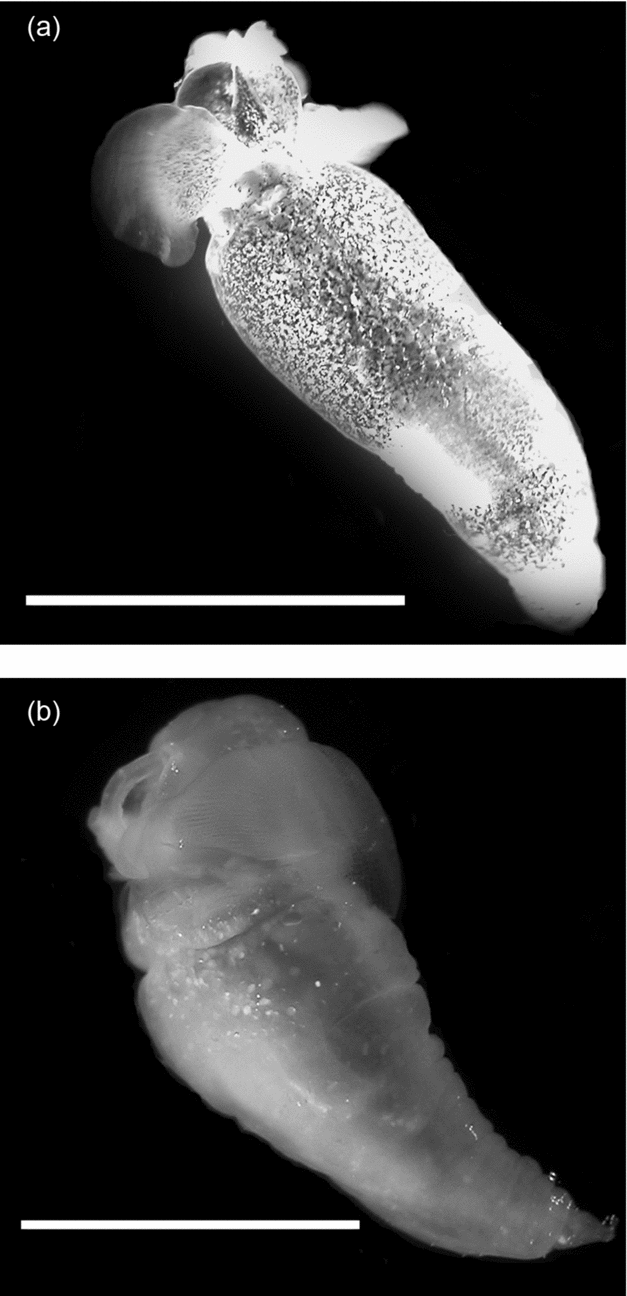
One of the unusual characteristics of the western Antarctic Peninsula (WAP) is the persistent intrusion of warmer Upper Circumpolar Deep Water (UCDW; Klinck and others Reference Klinck, Hofmann, Beardsley, Salihoglu and Howard2004; Martinson and others Reference Martinson, Stammerjohn, Iannuzzi, Smith and Vernet2008). UCDW flows at mid-depths (200 to 400 m) from the Antarctic Circumpolar Current (ACC), and creates a unique marine environment at mid-depths along the WAP as it intrudes into cross-shelf troughs where it mixes with colder coastal waters (for example Antarctic Surface Water (AASW) and Winter Water (WW); Smith and others Reference Smith, Ainley, Baker, Domack, Emslie, Fraser, Kennett, Leventer, Mosley–Thompson, Stammerjohn and Vernet1999a). The mixing influences water column structure and species’ composition for both vertebrate and invertebrate communities (Donnelly and Torres Reference Donnelly and Torres2008; Parker and others Reference Parker, Donnelly and Torres2011). For zooplankton such as the sub-Antarctic gymnosome Spongiobranchaea australis (Fig. 1a; d'Orbigny 1836) that is more commonly found north of the Polar Front (PF), or the Antarctic gymnosome Clione antarctica (Fig. 1b; Smith Reference Smith and Franklin1902) that lives at temperatures near −1.8°C south of the PF (Seibel and others Reference Seibel, Dymowska and Rosenthal2007), temperature has enormous potential for influencing their distributional ranges along the WAP (Hunt and others Reference Hunt, Pakhomov, Hosie, Siegel, Ward and Bernard2008).

Fig. 1. Southern Ocean gymnosomatous pteropods with a one cm scale bar: a) Spongiobranchaea australis, and b) Clione antarctica.
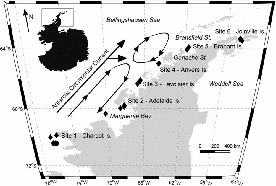
However, few studies have considered the distributions of these two gymnosomes along the WAP and south of the Gerlache Strait (for example Hopkins Reference Hopkins1985, U.S. Antarctic Marine Living Resources (AMLR) reports), a meso-scale region where the majority of UCDW enters onto the WAP shelf from the ACC (Fig. 2; Smith and others Reference Smith, Ainley, Baker, Domack, Emslie, Fraser, Kennett, Leventer, Mosley–Thompson, Stammerjohn and Vernet1999a, Klinck and others Reference Klinck, Hofmann, Beardsley, Salihoglu and Howard2004, Dinniman and others Reference Dinniman, Klinck and Hofmann2012). Hunt and others (Reference Hunt, Pakhomov, Hosie, Siegel, Ward and Bernard2008) reviewed decades of Antarctic gymnosome distribution data determined from various trawling methods, and reported that S. australis was essentially absent along the WAP during the months of March and April, whereas C. antarctica was consistently present throughout the year. Recently, Loeb and Santora (in press) revealed that the abundance of S. australis increases with climate change related to La Niña and intensified influence of the ACC. With increased UCDW and regional warming along the WAP (Meredith and King Reference Loeb and Santora2005; Ducklow and others Reference Ducklow, Baker, Martinson, Quetin, Ross, Smith, Stammerjohn, Vernet and Fraser2007; Martinson Reference Martinson2012), ecological studies can provide a better understanding of alterations occurring within this marine ecosystem, and gymnosomes may have sentinel species that indicate regional climate changes in the Bellingshausen Sea to the northern extent of Joinville Island (for example Comeau and others Reference Comeau, Gorsky, Jeffree, Teyssie and Gattuso2009, Reference Comeau, Jeffree, Teyssie and Gattuso2010; Lischka and others Reference Lischka, Budenbender, Boxhammer and Riebesell2011; Maas and others Reference Maas, Elder, Dierssen and Seibel2011a, Reference Maas, Elder, Dierssen and Seibel2011b; Seibel and others Reference Seibel, Maas and Dierssen2012).
Determining gymnosome distributions along the WAP requires a method of collecting multiple vertically or horizontally stratified zooplankton samples along a wide latitudinal range while also collecting data on the corresponding physical environment. And, as gymnosomes most often inhabit offshore waters, they are generally inaccessible unless sampled from research vessels equipped with plankton nets. Continuous Plankton Recorders damage soft tissues. Sediment traps, vital for understanding population dynamics of small plankton such as diatoms, planktonic foraminifers, and thecosomes (shelled pteropods), are not appropriate for soft-bodied organisms such as gymnosomes because preservatives deform key taxonomic features used for identification. In contrast, mesh nets of zooplankton samplers such as the Multiple Opening and Closing Net and Environmental Sampling System (MOCNESS) have been successfully used to sample a wide range of taxa without damage and in a variety of oceanic ecosystems when used aboard research vessels to capture live specimens. Another distinct attribute of the MOCNESS, relative to other mesh-net zooplankton sampler systems, is its ability to collect multiple vertically and horizontally stratified samples along with corresponding data on the immediate physical environment. Therefore the MOCNESS is a preferred sampling system to determine gymnosome distributions along the WAP.
In the present study, we postulated that distributions of S. australis and C. antarctica are determined by distinct water masses along the WAP. To test this hypothesis we looked for significant differences in gymnosome species distribution within and between sites, nets (depth strata), seawater temperatures, seawater salinities, seawater densities, latitudes (as they relate to the circulation of Antarctic water masses) as well as with oceanographic remotely sensed data. Our data summarise distributions of gymnosomes with depth (vertical distributions), among sites (horizontal distributions), and suggests that S. australis is more abundant in warmer waters influenced by UCDW advected from the ACC, while C. antarctica is more abundant at higher latitudes influenced by colder coastal water masses of the high Antarctic marine ecosystem.
Materials and methods
Hydrographic data sources
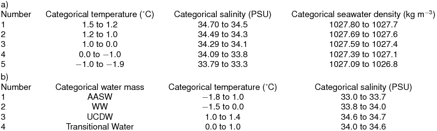
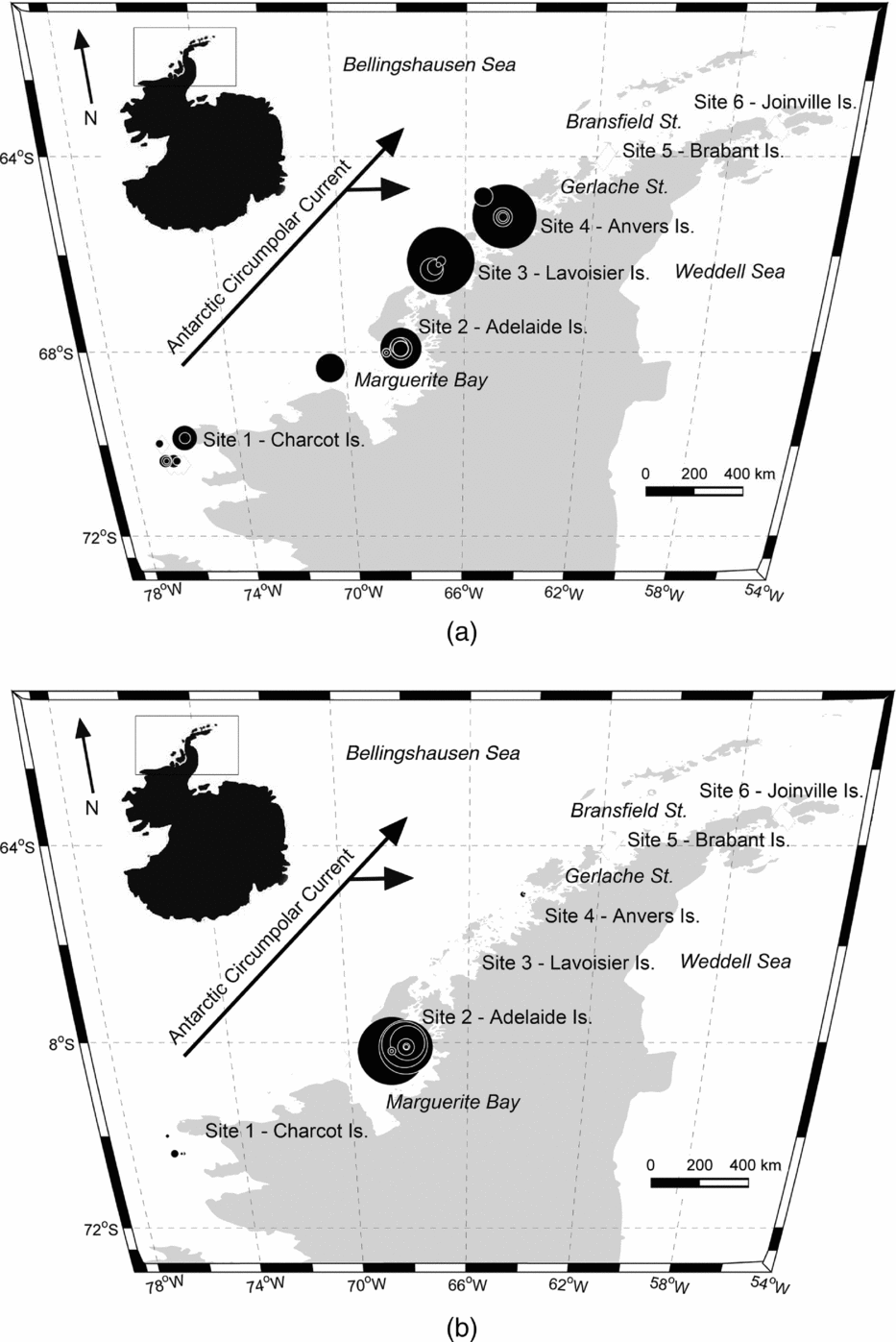
Hydrographic data collection corresponded with trawling events along the WAP, extending from Charcot Island in the south to Joinville Island in the north (Fig. 2, sites 1 to 6, respectively) during March and April 2010. Conductivity-temperature-depth (CTD) casts (n = 34) from Nathaniel B. Palmer utilised SeaBird SBE-45 and SeaBird 3–01/S instruments to record hydrographic data to depths approximately 50 m from the bottom. Seawater depth, temperature, and salinity data were post-processed for the downcast only. Post-processing utilised SeaBird software (SBEDataProcessing-Win 32) and seawater density was calculated using the UNESCO (1981)/Millero and Poisson (Reference Millero and Poisson1981) equations that use observed seawater temperatures and salinities. Southern Ocean water masses were identified using the seawater temperature and salinity guidelines from Smith and others (Reference Smith, Ainley, Baker, Domack, Emslie, Fraser, Kennett, Leventer, Mosley–Thompson, Stammerjohn and Vernet1999a): AASW temperatures 1.8 to 1.0°C with salinities ranging from 33.0 to 33.7 PSU, WW temperatures range down to −1.5°C with salinities ranging from 33.8 to 34.0 PSU, and UCDW temperatures 1.0 to 1.4°C with salinities ranging from 34.6 to 34.7 PSU.
Fig. 2. Western Antarctic Peninsula (WAP) with inset map denoting sampling area. Black diamonds in sites 1 to 6 represent locations of the 10 m2 Multiple Opening and Closing Net and Environmental Sampling System (MOC-10) trawls. Circulation of the Antarctic Circumpolar Current and sub-gyres 400 to 200 m along the WAP are adapted from Smith and others (Reference Smith, Ainley, Baker, Domack, Emslie, Fraser, Kennett, Leventer, Mosley–Thompson, Stammerjohn and Vernet1999a), and denoted by arrows.
Gymnosome sampling
Instrumentation mounted on the MOCNESS measured the volume of seawater filtered (m3 min−1) and depth (m) for each trawling event. Onboard instrumentation recorded all MOCNESS readings, as well as the latitude and longitude of the trawling event and trawling speed. On occasions when the flow volume instrumentation failed for an individual MOCNESS net, volume of water filtered in the net was estimated based on cruise-wide mean volumes filtered per minute per depth stratum, trawl duration, and speed.
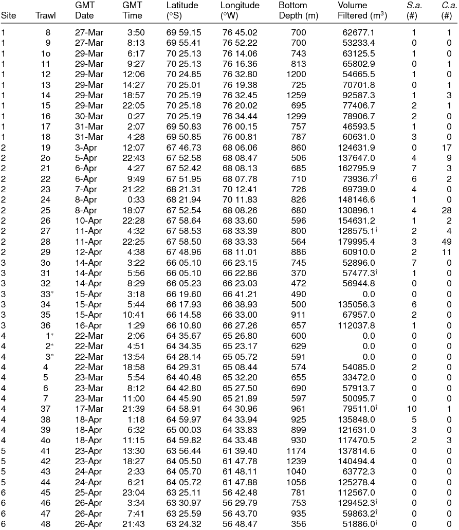
Gymnosomes were collected from MOCNESS trawls in deep shelf waters along the cruise track. A 10 m2 MOCNESS (MOC-10) fitted with 3 mm mesh nets and capable of collecting vertically stratified samples was used (Wiebe and others Reference Wiebe, Burt, Boyd and Morton1976, Reference Wiebe, Morton, Bradley, Backus, Craddock, Barber, Cowles and Flierl1985; Donnelly and Torres Reference Donnelly and Torres2008; Parker and others Reference Parker, Donnelly and Torres2011). Five discrete depth layers between 0 to 500 m were sampled. The initial, or drogue net, trawled obliquely to 500 m with subsequent nets sampling 500 to 300 m (net 1), 300 to 200 m (net 2), 200 to 100 m (net 3), 100 to 50 m (net 4), and 50 to 0 m (net 5). MOC-10 trawls were performed throughout the day and night, with towing speeds ranging from 1.5 to 2.5 knots. Upon retrieval, contents collected in each MOC-10 net were emptied into 19L buckets, and the gymnosomes present in each bucket were removed, enumerated, and identified to species level. Results were expressed as density of gymnosomes captured (number per 104 m−3 volume of seawater filtered; Donnelly and Torres Reference Donnelly and Torres2008). A total of 44 trawls were made: 11, 11, 6, 8, 4 and 4, from sites 1–6, respectively.
Main goals of the field work required nearly exclusive use of the MOC-10 at each site. However, at each of the six sites at least one 1 m2 MOCNESS (MOC-1) trawl was taken using nine, 333 μm mesh nets, primarily for archival purposes. MOC-1 trawls confirmed that adult gymnosomes were present only in sites 1 to 4.
Oceanographic remote sensing data
Oceanographic remotely sensed data used in this study were obtained from the Giovanni online data system developed and maintained by the NASA GES DISC at http://giovanni.gsfc.nasa.gov (Berrick and others Reference Berrick, Leptoukh, Farley and Rui2009), and from the National Snow and Ice Data Center online data system and produced by P. Gloersen, NASA/GSFC, Oceans and Ice Branch. Giovanni MODIS-Aqua data at a 4 km resolution were obtained from Ocean Portal's Ocean Color Radiometry Online Visualization and Analysis global monthly products. MODIS-Aqua data were averaged for each month, March and April 2010, and then compared to trawling events occurring in their respective month. These data included coloured dissolved organic matter (CDOM), chlorophyll concentration (CHLO), normalised fluorescence line height (NFLH), nighttime sea surface temperature (NSST), photosynthetically active radiation (PAR), particulate inorganic carbon (PIC), particulate organic carbon (POC), and daytime sea surface temperature (SST). NASA GES DISC defines particulate matter as particles that are caught by filter with pore size 0.7 μm, while dissolved matter are eluted through the filter. POC largely consists of phytoplankton and organic detritus and PIC consists primarily of biogenic calcium carbonate; they are both estimated using remote sensing through backscatter algorithms. NFLH is solar-stimulated chlorophyll a fluorescence at 698 nm. Daily sea-ice concentration (DSIC) data over this study's sampling area were generated using the NASA team algorithm (Cavalieri and others Reference Cavalieri, Parkinson, Gloersen and Zwally1996; Nimbus-7 SMMR and DMSP SSM/I passive microwave data), then compared to trawling events occurring on associated days. Remotely sensed data were matched with species’ density data using latitude and longitude coordinates to the nearest tenth of a decimal degree. For a point of latitude and longitude correlating to species’ density that had no comparable oceanographic data, two-dimensional linear interpolation was performed using Delaunay triangulation of the scattered data (Matlab: MathWorks, Natick, Massachusetts, USA; de Berg and others Reference de Berg, Cheong, van Kreveld and Overmars2008).
Statistical methods
Statistical analyses were performed in Matlab with the Fathom toolbox (Jones Reference Jones2012) to include a distribution free, permutation-based variant of MANOVA (NP-MANOVA; Anderson Reference Anderson2001), which is appropriate for analysing ecological data. For analyses, CTD cast profiles of seawater temperature, salinity and density were averaged in 10 m intervals, as each CTD cast varied in depth and could not be directly compared per trawling event. Significance for each statistical method (P < 0.05) was evaluated with distribution-free randomization tests (n = 1000 iterations), removing reliance on the assumptions of any one distributional model (Anderson Reference Anderson2001).
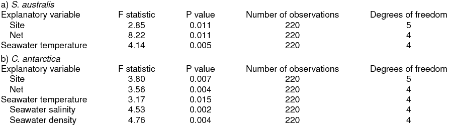
NP-MANOVA was used to analyse vertical density data for both species, accounting for presence and absence per trawl, per net, in relation to the categorical variables site, net, and seawater temperature, salinity, and density (Table 1a), and the Southern Ocean water masses, AASW, WW, UCDW and warm transitional waters influenced by UCDW (Table 1b). The first set of null hypotheses stated that there were no differences in gymnosome densities among levels of the independent categorical variables. When an explanatory variable yielded a significant effect, NP-MANOVA was followed by post-hoc multiple comparison pair-wise tests.
Table 1. Categorical transformation ranges for temperature, salinity and density
Analyses also included a stepwise forward selection of explanatory variables in Redundancy Analysis (RDA) based on Akaike information criterion (AIC) to explain variability in gymnosome vertical density per stratified trawling event. To find the most parsimonious subset of the explanatory variable(s) using RDA, the following categorical variables were used: site, net, mean net depth of occurrence, water mass, seawater temperature, salinity, density, and trawl latitude and longitude. Calculating the mean net depth of occurrence for gymnosomes captured in the MOC-10 trawls was accomplished using the Matlab Fathom toolbox to calculate a weighted mean depth of occurrence separately for all sites and for each sampling event (f_depthMean; Brodeur and Rugen Reference Brodeur and Rugen1994). Latitude and longitude were converted to Universal Transverse Mercator (UTM) coordinates for Northing and Easting. Categorical variables were dummy coded when used in RDA. Continuous explanatory variables were transformed using square root, fourth root, log base ten (x + 1), natural log (x + 1), and log base two (x + 1). For the response data, the vertical density of gymnosomes had only square root and fourth root transformations applied. The second set of null hypotheses stated that there were no relationships between gymnosome vertical densities and the categorical variables site, net, mean net depth, water mass, temperature, salinity, density, and Northing and Easting.
Horizontal abundance data (number of gymnosomes under 103 m2 of sea surface) were calculated by summing the total gymnosomes caught per trawling event over the trawling area (Goldman and McGowan Reference Goldman and McGowan1991; Criales and others Reference Criales, Paris, Yeung, Jones, Richards and Lee2004) then analysed with NP-MANOVA to test for a separation of distributions between sampling sites. When significance differences were detected, post-hoc multiple comparison pair-wise tests were used to detect where there were significant effects in relation to gymnosome horizontal abundances and site. The third null hypothesis stated that there was no difference in gymnosome horizontal abundance in regards to site.
Analyses also included a stepwise forward selection of explanatory variables in RDA based on AIC to explain the variability of only known gymnosome density per stratified trawling event. This was done to find the most parsimonious subset of the explanatory variable(s) in RDA to explain observed gymnosome density in regards to the following explanatory variables: site, net, mean net depth, Southern Ocean water mass type (per Smith and others Reference Smith, Ainley, Baker, Domack, Emslie, Fraser, Kennett, Leventer, Mosley–Thompson, Stammerjohn and Vernet1999a), seawater temperature, seawater salinity, seawater density, latitude, longitude, and remotely sensed data. Prior to statistical analyses latitude and longitude coordinates were converted to UTM coordinates to Northing and Easting. Categorical explanatory variables were dummy coded when used in RDA. Continuous explanatory variable data was transformed using square root, fourth root, log base ten (x + 1), natural log (x + 1), and log base two (x + 1). For the response data, vertical density of gymnosomes had only square root and fourth root transformations applied. The fourth set of null hypotheses stated that there were no relationships between gymnosome vertical densities and the categorical variables site, net, mean net depth, Southern Ocean water mass type, temperature, salinity, density, Northing, Easting, and the remotely sensed data.
Results
Sampling sites and hydrography
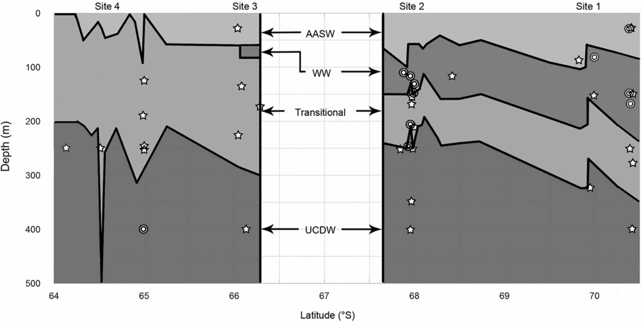
Temperature-salinity profiles from the CTD cast data reveal the presence of WW in the southernmost sampling sites, 1 and 2, while WW was almost entirely absent from site 3, and completely absent in site 4 (Fig. 3). The near absence of WW at sites 3 and 4 suggests that this water mass was mixed with the warmer waters from the ACC, creating warmer transitional waters at mid depths. AASW, transitional water, and UCDW were consistently detected in sites 1 to 4. The more northern sites 5 and 6 had nearly isothermal water columns and individual water masses were not present. For this reason, and concerning the gymnosome capture data below, hydrographic results focus on sites 1 to 4 only. Temperatures at sites 1 through 4 were typically above 0°C, whereas temperatures at sites 5 and 6 were typically below 0°C. For this study the water temperature minimum was approximately −1.8°C, and the maximum was approximately 1.8°C.
Fig. 3. Water masses and gymnosome depths. Water masses identified for sites 1 to 4, as determined by CTD casts, are illustrated by latitude and water depth (left y-axis). Water mass boundaries at depth are denoted by solid black lines. Water masses labeled are: Antarctic Surface Water (AASW), Winter Water (WW), Transitional Water, and Upper Circumpolar Deep Water (UCDW). Mixing is assumed to create the Transitional Water's temperatures and salinities. Mean depths of capture of gymnosomes per trawl by latitude are illustrated for S. australis with open stars, and C. antarctica double open circles.
Mean hydrographic data (Fig. 3) revealed a seawater profile in site 1 with AASW extending from the surface to 70 m, WW from 70 to 130 m, warmer transitional waters from 130 to 260 m, and UCDW from 260 to 500 m; site 2 with AASW from surface to 70 m, WW from 70 to 110 m, warmer transitional waters from 110 to 220 m, and UCDW from 220 to 500 m; and site 3 and site 4 lost the colder mid-depth waters. Site 3 had AASW from the surface to 60 m, warmer transitional waters from 60 to 300 m, and UCDW from 300 to 500 m. However a very small presence of WW from 40 to 60 m near 66°S in site 3 was revealed in CTD cast data. Site 4 had AASW from surface to 70 m, warmer transitional waters from 70 to 230 m, and UCDW from 230 to 500 m. The water column structure indicates a consistent presence of UCDW in each of the sites, with the majority of the warmer UCDW detected in sites 3 and 4, or nearest to the ACC.
Species vertical density, horizontal abundance, and hydrography
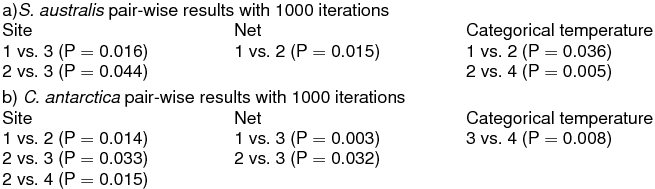
Adult gymnosomes were absent in stratified MOC-10 trawls in sites 5 and 6, sites characterised by isothermal water columns, while trawls at sites 1 to 4 consistently captured adult gymnosomes and CTD casts revealed stratified water columns. Across sites 1 to 4, S. australis was captured most often in the depth stratum of net 2, 300 to 200 m (Fig. 3). Cruise-wide mean water depth of occurrence for S. australis was 179 ± 18 m. The mean depth of capture at site 1 was 171 ± 42 m, site 2 was 174 ± 42 m, site 3 was 151 ± 32 m, and site 4 was 209 ± 33 m. The first series of null hypotheses were rejected as vertical densities of S. australis differed significantly by site and seawater temperature, and demonstrated a relationship with deeper water strata (net 2) associated with warmer water temperatures (Table 2a). Pair-wise test results for S. australis demonstrated significant vertical density differences in site 3 as compared to sites 1 and 2, net 2 compared to net 1, and temperature ranging from 1.2 to 1.0°C versus 1.5 to 1.2 or 0.0 to −1.0°C (Table 3). Pair-wise test results for both gymnosome species are shown in Table 4a.
Table 2. Significant NP-MANOVA results
Table 3. 10 m2 MOCNESS (MOC-10) trawl data for WAP Austral Fall cruise (2010)
Note: S.a. = Spongiobranchaea australis, C.a. = Clione antarctica
†Flow volume instrumentation failed for individual MOC-10 net, * Failed MOC-10 tow
Table 4. Pairwise results; P < 0.05 is considered significant
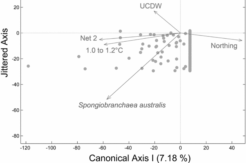
Spongiobranchaea australis was captured most often in warmer transitional waters influenced by UCDW or in UCDW. The second null hypothesis was rejected as vertical density differences across sites 1 to 4 is explained by a negative relationship with latitude (Northing), a strong positive relationship with depths sampled by net 2, a positive relationship with warmer water temperatures (1.2 to 1.0°C) indicative of transitional water influenced by UCDW, and a positive relationship with UCDW when plotted on a single canonical axis (RDA:Fig. 4; F = 3.34, P = 0.008, N = 180 obs.). Therefore, higher vertical densities of S. australis were associated with lower latitudes, UCDW, warmer water temperatures, and the 300 to 200 m depth stratum sampled by Net 2. Horizontal abundances for this species showed no significant differences among sites 1 through 4 per our third null hypothesis, although the abundance of S. australis generally increased moving from site 1 to site 4 (Fig. 5a).
Fig. 4. Redundancy analysis (RDA) plot for S. australis with respect to water masses and water mass properties. RDA reveals a negative relationship with latitude (Northing), a strong positive relationship with depths sampled by net 2 (300–200m), and a positive relationship with Upper Circumpolar Deep Water (UCDW) when plotted on a single canonical axis (RDA: F = 4.39, P = 0.004, N = 180 obs.). Higher vertical densities of S. australis were associated with lower latitudes, UCDW, warmer water temperatures, and the 300 to 200 m depth stratum sampled by Net 2.
Fig. 5. Distribution bubble plots of a) S. australis and b) C. antarctica across study sampling area. Bubbles produced using numbers of gymnosomes captured (104 m3) per volume of seawater filtered (m3; Table 3) in 10 m2 Multiple Opening and Closing Net and Environmental Sampling System (MOC-10) trawling events (n = 44) with respect to latitude and longitude. Bubbles are proportional to the range of densities of gymnosomes captured along the western Antarctic Peninsula, and larger bubbles indicate greater densities. S. australis was captured more frequently per trawl in sites closer to the Antarctic Circumpolar Current (sites 3 and 4), whereas C. antarctica was primarily caught in Marguerite Bay (site 2).
In contrast, C. antarctica was rarely captured anywhere except for site 2 (Fig. 3, Table 3). This species was captured most often in the depth stratum 200 to 100 m, net 3 (Fig. 3). Cruise-wide mean depth of occurrence was 135 ± 9 m. The mean depth of capture at site 1 was 100 ± 29 m, site 2 was 137 ± 9 m, site 3 trawls captured no C. antarctica, and in site 4 was 288 ± 43 m. The first set of null hypotheses were rejected for this species as vertical densities differed significantly by site, a more shallow water strata sampled by net 3, seawater temperature, seawater salinity, and seawater density (Table 2b). Pair-wise test results for C. antarctica demonstrated significant vertical density differences in site 2 as compared to either site 1, 3 or 4, in net 3 compared to nets 1 or 2, and temperature ranging from 0.0 to −1.0°C versus 1.0 to 0.0°C (Table 4b).
In general vertical densities of C. antarctica were most strongly associated with cooler water temperatures in more shallow waters. The second null hypothesis was rejected as C. antarctica vertical density variability across sites 1 to 4 is explained by a strong relationship with cold temperatures relating to WW (−1.0 to 0.0°C), a strong relationship with site 2, a weaker relationship with seawater salinities influenced by AASW (33.3 to 33.8 PSU), and a negative relationship with UCDW when plotted on a single canonical axis (Fig. 6; RDA: F = 12.03, P = 0.001, N = 180 obs.). Therefore, higher vertical densities of C. antarctica were associated with a decreased presence of UCDW, less saline waters, proximity to site 2, and cold water temperatures relating to WW. C. antarctica's horizontal abundances were significantly different between sites (NP-MANOVA: F = 3.75, P = 0.016, N = 36 obs.), with pairwise tests showing significant separations in site 2 versus 3 (P = 0.050) and in site 2 versus 4 (P = 0.030). The third null hypothesis was rejected as C. antarctica's horizontal abundances varied with latitude, with the greatest horizontal abundances observed in the southernmost sites (Fig. 5b).
Fig. 6. Redundancy analysis (RDA) plot for C. antarctica with respect to water masses and water mass properties. RDA reveals a strong relationship with cold temperatures relating to WW (-1.0 to 0.0°C), a strong relationship with site 2, a weaker relationship with salinities relating to AASW (33.3 to 33.8 PSU), and a negative relationship with Upper Circumpolar Deep Water (UCDW) when plotted on a single canonical axis (RDA: F = 12.03, P = 0.001, N = 180 obs.). Higher vertical densities of C. antarctica were associated with a decreased presence of UCDW, less saline waters, proximity to site 2, and cold water temperatures relating to WW.
RDA analysis of gymnosome densities under the fourth hypothesis confirmed the relationships with Southern Ocean water masses and depth, however C. antarctica density also demonstrated a positive relationship with the presence of sea ice. The fourth null hypothesis was rejected for S. australis as 60% of the variability in vertical density across sites 1 to 4 was explained by a strong relationship with transitional waters influenced by UCDW and deeper depths (Fig. 7a; RDA: F = 15.80, P = 0.001, N = 35 obs.). The fourth null hypothesis was also rejected for C. antarctica as 69% of the variability in vertical density across sites 1 to 4 was explained by a strong relationship with site 2, a weak negative relationship with sea ice, and a negative relationship with AASW (Fig. 7b; RDA: F = 23.37, P = 0.001, N = 35 obs.). Therefore vertical densities of S.australis increase in warmer, deeper waters, whereas vertical densities of C. antarctica increase closer to site 2 and decreases with the presence of sea ice and AASW.
Fig. 7. Redundancy analysis (RDA) plot for a) S. australis, and b) C. antarctica when including oceanographic remotely sensed variables. S. australis’ vertical densities across sites 1 to 4 reveals a strong relationship with transitional waters influenced by UCDW and deeper depths related to UCDW (RDA: Fig. 6a, F = 15.80, P = 0.001, N = 35 obs.), whereas C. antarctica's vertical densities across sites 1 to 4 reveals a strong relationship with site 2, a weak negative relationship with sea ice, and a negative relationship with AASW (RDA: Fig. 6b, F = 23.37, P = 0.001, N = 35 obs.). Therefore vertical densities of S. australis increase in warmer, deeper waters, whereas vertical densities of C. antarctica increase closer to site 2 and with the presence of sea ice, but decreases with the increasing presence of AASW.
Discussion
Gymnosome distributions were influenced primarily by Southern Ocean water masses, temperature, site, depth, and latitude along the WAP. The highest densities of S. australis were associated with lower latitudes nearest the ACC and warmer water temperatures influenced by advection of UCDW from the ACC in the 300 to 200 m depth stratum. In contrast, the highest vertical densities of C. antarctica were associated with less saline, colder waters in site 2, and vertical density generally decreased in the presence of UCDW and further from the ACC. The present study's hydrographic data revealed that UCDW has increased its influence at depth on the WAP marine ecosystem since the study of Smith and others (Reference Smith, Ainley, Baker, Domack, Emslie, Fraser, Kennett, Leventer, Mosley–Thompson, Stammerjohn and Vernet1999a), which is confirmed by Dinniman and others (Reference Dinniman, Klinck and Hofmann2012). More S. australis were observed in sites 3 and 4, sites that experience the most intrusions of UCDW at depth.
Comparisons of the present study's hydrographic data with that of Smith and others (Reference Smith, Ainley, Baker, Domack, Emslie, Fraser, Kennett, Leventer, Mosley–Thompson, Stammerjohn and Vernet1999a) showed similar vertical water temperature minima in shelf waters along the WAP for the autumn, yet the present study's temperature maxima were approximately 0.5°C warmer. Increasing UCDW intrusions originating from ACC are consistent with the observed warming trend. The topographical relief, 200 m relative to 400 m, for the continental shelf waters of the WAP facilitate the formation of a large cyclonic gyre bound between the ACC and Antarctic continent within the Bellingshausen Sea. Within this gyre are two cyclonic sub-gyres that circulate UCDW into WAP shelf waters at depth. The dynamic forces of the sub-gyres direct the greatest amounts of UCDW from the ACC into WAP shelf waters near sites 3 and 4 (Fig. 2; Dinniman and others Reference Dinniman, Klinck and Hofmann2012). The depths of the dynamic topography (400 to 200 m) are considered to be below the influence of seasonal variability (Hofmann and others Reference Hofmann, Lascara and Klinck1992, Reference Hofmann, Klinck, Lascara, Smith, Ross, Hofmann and Quetin1996; Smith and others Reference Smith, Ainley, Baker, Domack, Emslie, Fraser, Kennett, Leventer, Mosley–Thompson, Stammerjohn and Vernet1999a), and therefore increased UCDW and warmer water temperatures at depth indicates long-term and sustained water mass warming in this polar marine ecosystem with the advection of warm water masses from the ACC.
Interestingly, temperatures below 200 m along the WAP have not only increased, but warmer water temperatures have also progressed landward over the last two decades since the Smith and others (Reference Smith, Ainley, Baker, Domack, Emslie, Fraser, Kennett, Leventer, Mosley–Thompson, Stammerjohn and Vernet1999a) observations, as revealed in the present study's CTD data. The increased UCDW intrusions, and thus warmer waters along the WAP shelf, could be affected by interannual or decadal-scale variations. However, our results are also confirmed by the WAP hydrographic data of Martinson and others (Reference Martinson, Stammerjohn, Iannuzzi, Smith and Vernet2008), Dinniman and others (Reference Dinniman, Klinck and Hofmann2012), and Martinson (Reference Martinson2012) who reported a persistent warming of WAP shelf waters with an increasing presence of UCDW over the recent decades. Martinson (Reference Martinson2012) also reported increases in UCDW along the WAP, which is likely the result of westerly wind intensification, increased UCDW upwelling and decreased seasonal sea ice (Dinniman and others Reference Dinniman, Klinck and Hofmann2012). Westerly wind intensification around Antarctica has increased 20% since the 1970s (Trathan and others Reference Trathan, Fretwell and Stonehouse2011; Dinniman and others Reference Dinniman, Klinck and Hofmann2012), influencing UCDW advection from the ACC. Upwelling of UCDW is most pronounced near Lavoisier and Anvers Islands south of the Gerlache Strait (Klinck and others Reference Klinck, Hofmann, Beardsley, Salihoglu and Howard2004; Smith and others Reference Smith, Hofmann, Klinck and Lascara1999b; Dinniman and others Reference Dinniman, Klinck and Hofmann2012). The persistent warming at depth by UCDW has created a shifting mesoscale temperature gradient along the WAP marine ecosystem, as warmer waters continue to move landward, ultimately affecting species’ distributions (for example Moline and others Reference Moline, Claustre, Frazer, Schofield and Vernet2004).
Where the greatest amounts of UCDW entered the WAP shelf waters at depth near Lavoisier and Anvers Islands, the highest densities of S. australis were found. And, as UCDW was continually present at depth in sampling sites 1 to 4, so was S. australis. Moving southward to the colder waters at sites 1 and 2, a significant increase in C. antarctica densities and abundances were observed; particularly in site 2. Both of these sites were influenced by WW, and both sites contained C. antarctica.
The present study demonstrates a distributional range for S. australis further south of the PF than the range reported in Hunt and others (Reference Hunt, Pakhomov, Hosie, Siegel, Ward and Bernard2008) and in the reviewed studies over the last three decades cited therein. Since these earlier studies, the WAP has experienced a diminishing seasonal sea-ice cover and a subsequent highly altered seasonal cycle, ultimately resulting in the distributional shifts of polar marine organisms (Fraser and others Reference Fraser, Trivelpiece, Ainley and Trivelpiece1992; Rott and others Reference Rott, Skvarca and Nagler1996; Trivelpiece and Fraser Reference Trivelpiece, Fraser, Ross, Hofmann and Quetin1996; Smith and others Reference Smith, Baker and Stammerjohn1998; McClintock and others Reference McClintock, Ducklow and Fraser2008; Moline and others Reference Moline, Karnovsky, Brown, Divoky, Frazer, Jacoby, Torres and Fraser2008; Lawson and others Reference Lawson, Wiebe, Ashjian and Stanton2008; Convey and others Reference Convey, Bindschadler, di Prisco, Fahrbach, Gutt, Hodgson, Mayewski, Summerhayes, Turner and Consortium2009). For example, with diminishing seasonal sea-ice cover the ice-dependent Adélie penguin populations have significantly decreased, and ice-intolerant chinstrap and gentoo penguin populations have increased (Smith and others Reference Smith, Hofmann, Klinck and Lascara1999b, Ducklow and others Reference Ducklow, Baker, Martinson, Quetin, Ross, Smith, Stammerjohn, Vernet and Fraser2007). Synchronously, the ice-dependent Antarctic silverfish (Pleuragramma antarcticum), a keystone species in the polar pelagic marine ecosystem, has been disappearing along the WAP (Ducklow and others Reference Ducklow, Baker, Martinson, Quetin, Ross, Smith, Stammerjohn, Vernet and Fraser2007). Recent warming of the WAP marine ecosystem at depth (400 to 200 m) has also increased the biomass of ice-intolerant species of sponges and bryozoans (Barnes and others Reference Barnes, Webb and Linse2006; Aronson and others Reference Aronson, Thatje, Clarke, Peck, Blake, Wilga and Seibel2007).
As with other distributional shifts due to WAP warming, S. australis may have expanded its distributional range into increasingly habitable waters south of the PF, made possible by the increasing water mass advection of UCDW from the ACC, while distributions of C. antarctica are restricted to more southern regions. When comparing the present study's MOC-10 data from sites 2 and 3 to the 2001–2002 autumn MOC-10 Global Ocean Ecosystem Dynamics (GLOBEC) data on gymnosome densities at the corresponding sites reported in Parker and others (Reference Parker, Donnelly and Torres2011), we found that S. australis was again influenced by waters advected from the ACC, as well as an increasing high latitude density of C. antarctica in site 2. For example, S. australis was never captured in the GLOBEC Fall 2001 MOC-10 trawling events. In 2002 trawls S. australis was captured most often in more northern waters near the ACC, and proximity to the ACC increased the mean density of S. australis, explaining 22% of the variability in distributions reported in Parker and others (Reference Parker, Donnelly and Torres2011; RDA: F = 6.78, P = 0.026). Mean density of S. australis in site 2 increased from 0.008 to 0.380 gymnosomes per 104 m−3 of seawater, from 2002 to 2010, respectively. In the GLOBEC autumn 2002 MOC-10 trawls S. australis was absent in site 3, yet this study's 2010 mean density in site 3 increased substantially to 0.74 gymnosomes per 104 m−3 of seawater. C. antarctica's 2002 to 2010 mean density in site 2 increased from 0.02 to 1.26 gymnosomes 104 m-3 of seawater, and was also absent in site 3 in 2001, 2002 and 2010 MOC-10 trawls. The observed changes in mean autumn density of C. antarctica from 2001 to 2002 are similar to shifts in krill distributions, a probable response to warmer water masses along the WAP (Lawson and others Reference Lawson, Wiebe, Ashjian and Stanton2008).
Warmer water temperature would affect metabolic rates and enzymatic activities, ultimately influencing the ability of organisms to forage, reproduce, and/or avoid predation (Pörtner and others Reference Pörtner, Peck and Somero2007). The Antarctic polar marine ecosystem is generally characterised by permanently cold, stable temperatures (Clarke and Peck Reference Clarke and Peck1991), and as a tradeoff for life adapted to these low temperatures, there is a decreased tolerance of changing temperatures (Clarke Reference Clarke1998; Pörtner and others Reference Pörtner, Peck and Somero2007). Although there are no studies detailing the physiology of the sub-Antarctic gymnosome S. australis, its typical habitat characteristics north of the PF and this study's distribution correlations suggest that S. australis is physiologically adapted to warmer sub-polar temperatures and water masses. As warmer water masses are increasingly advected from the ACC onto the WAP shelf, S. australis populations may be able to expand their distributions in the region of the WAP.
Physiological studies of C. antarctica reveal neuro-muscular and energetic temperature compensation that supports its continuous locomotion in cold waters (Seibel and others Reference Seibel, Dymowska and Rosenthal2007; Rosenthal and others Reference Rosenthal, Seibel, Dymowska and Bezanilla2009; Dymowska and others Reference Dymowska, Manfredi, Rosenthal and Seibel2012). It is likely that the dissimilar habitats of the Southern Ocean gymnosomes have resulted in different physiological adaptations to live in distinct thermal ranges or ‘climate envelopes’ (Pearson and Dawson Reference Pearson and Dawson2003). One line of evidence to support this theory comes from the visual observations during the present study, which suggest that the sub-Antarctic S. australis may have two swimming gaits. Observations at 0°C in the present study revealed that over the small range S. australis possessed an escape response with a wing-beat frequency of approximately 1.9 Hz, whereas C. antarctica maintained a wing-beat frequency of approximately 1.4 Hz. It is thought that the sub-Antarctic gymnosome S. australis possesses a greater scope for locomotor activity than the Antarctic gymnosome C. antarctica.
If Southern Ocean gymnosomes live in dissimilar thermal ranges, colder Antarctic waters would act as a physiological barrier to limit the distributions of S. australis, and similarly, warmer temperatures would act as a physiological barrier to limit the distributions of the cold-adapted C. antarctica (Seibel and others Reference Seibel, Dymowska and Rosenthal2007; Pörtner and others Reference Pörtner, Peck and Somero2007; Pörtner and Farrell Reference Pörtner and Farrell2008). Unique water masses of the Southern Ocean, defined by temperature and salinity, are invaluable mesoscale indicators of physical oceanography and the dynamic marine ecosystem response. With increasing occurrences of UCDW impinging upon the WAP shelves, temperature driven distributional shifts of both gymnosome species may increase future interactions, ultimately shifting distributions in a region changing from a polar environment to a sub-polar one (Roy and others Reference Roy, Jablonski, Valentine and Rosenberg1998; Ducklow and others Reference Ducklow, Baker, Martinson, Quetin, Ross, Smith, Stammerjohn, Vernet and Fraser2007; Martinson Reference Martinson2012).
Acknowledgements
The United States National Science Foundation supported this research (NSF ANT 0741348 to J.J.T.). Thank you to the University of South Florida (USF) science team aboard Nathaniel B. Palmer cruise, 10-02, for their help collecting MOCNESS samples (Christine Cass, Tammy Cullins, Nicole Dunham, Erica Ombres, Eloy Martinez, Christin Murphy, and Melanie Parker), and the vessel's crew for their help in collecting CTD data. Thank you to Dr. Pamela Hallock from USF - College of Marine Science from the University of South Florida for her editing and literary insights, as well as Melanie Parker for sharing 2001/2002 GLOBEC data.