


1 INTRODUCTION
In 1934, Hubble observed that the frequency distribution of the count of galaxies over the space is strongly skewed but the distribution of its logarithm is close to symmetric. Bok (Reference Bok1934) and Mowbray (Reference Mowbray1938) found that variance of the count is considerably larger than expected for a random galaxy distribution. Such studies indicates that locally galaxies are clustered over space. Several attempts have been made to study this clustering nature on the basis of angular positions of the galaxies. Most of them (Chandrasekhar & Munch Reference Chandrasekhar and Munch1952; Zwicky Reference Zwicky1953; Limber Reference Limber1953, Reference Limber1954) have used spatial and angular correlation functions to study this phenomenon. In this area, the contributions of Neyman, Scott, & Shane (Reference Neyman, Scott and Shane1954) is very significant. This spatial clustering nature motivated us to investigate the clustering nature with respect to the other parameters also by using the same approach.
Classical formation of elliptical galaxies can be divided into five major categories, e.g. (i) the monolithic collapse model (Larson Reference Larson1975; Carlberg Reference Carlberg1984; Arimoto & Yoshii Reference Arimoto and Yoshii1987), (ii) the major merger model (Toomre & Toomre 1972; Ashman & Zepf Reference Ashman and Zepf1992; Zepf et al. Reference Zepf2000; Bernardi et al. Reference Bernardi, Roche, Shankar and Sheth2011; Prieto et al. Reference Prieto2013), (iii) the multiphase dissipational collapse model (Forbes, Bordie, & Grillmair Reference Forbes, Bordie and Grillmair1997), (iv) the dissipationless merger model (Bluck, Conselice, & Buitrago Reference Bluck, Conselice and Buitrago2012; Newman et al. Reference Newman2012), and (v) the accretion and in situ hierarchical merging (Mondal, Chattopadhyay, & Chattopadhyay Reference Mondal, Chattopadhyay and Chattopadhyay2008). Recent observations in the deep field have explored that high redshift galaxies have the size of the order of 1 kpc (Daddi, Renzini, & Pirzkal Reference Daddi, Renzini and Pirzkal2005; Trujillo, Feulner, & Goranova Reference Trujillo, Feulner and Goranova2006; Damjanov, Abraham, & Glazebrook Reference Damjanov, Abraham and Glazebrook2011) and have higher velocity dispersion (Cappellari, di Serego Alighieri, & Cimatti Reference Cappellari, di Serego Alighieri and Cimatti2009; Onodera et al. Reference Onodera, Renzini and Carollo2012) than nearby early type galaxies (ETGs) of the same stellar mass. Galaxies at intermediate redshifts (since z ≈ 2.5) have stellar masses and sizes increased by a factor almost 3–4 (van Dokkum, Whitaker, & Brammer Reference van Dokkum, Whitaker and Brammer2010; Papovich, Bassett, & Lotz Reference Papovich, Bassett and Lotz2012; Szomoru, Franx, & van Dokkum Reference Szomoru, Franx and van Dokkum2012). All these evidences suggest that massive ETGs form in two phases viz. inside-out, i.e. intense dissipational process like accretion (Dekel, Sari, & Ceverino Reference Dekel, Sari and Ceverino2009) or major merger form, an initially compact inner part. After this a second slower phase starts when the outermost part is developed through non-dissipational process, e.g. dry minor merger. The above development arising both in the field of observations as well as theory, severely challenges classical models like, monolithic collapse or major merger and favours instead a ‘two phase’ scenario (Oser et al. Reference Oser2010; Johansson, Naab, & Ostriker Reference Johansson, Naab and Ostriker2012) of the formation of nearby elliptical galaxies. The task remains is to check whether the compact inner parts of the nearby ETGs have any kind of similarity with the fossil bodies (viz. ‘red nuggets’) at high redshift.
In a previous work (Huang et al. 2013b), the authors have pursued the above task through matching ‘median’ values of the two systems. They used this measure with respect to univariate data and the univariate data they considered, are either stellar ‘mass’ or ‘size’. For ETGs in the redshift range, 0.5 ⩽ z ⩽ 7, considered, in the present data set, the stellar mass–size correlation is r(M *, R e) = 0.391, p-value = 0.00. For nearby ETGs for inner, intermediate and outer components the stellar mass–size correlations with p-values are r(M *, R e) = 0.720, p-value = 0.00, r(M *, R e) = 0.636, p-value = 0.00, r(M *, R e) = 0.573, p-value = 0.00, respectively and all these values are highly significant. Hence, use of univariate median matching is not sufficient in the present context for highly correlated bivariate data. Also, median does not include all objects in a particular data set. For this a more sophisticated technique is in demand for such kind of investigation.
In the present work, we have used the mass–size data of high redshift galaxies and nearby ETGs and used a cross correlation, especially designed to study bivariate data. This is more trustworthy and meaningful in the present situation. In Section 2, we have discussed the data set and in Section 3, we have described the method. The results and interpretations are given under Section 4.
2 DATA SETS
We have considered eight data sets. Data sets 1–3 have been taken from Ho et al. (Reference Ho2011). In data sets 1–3 there are 70 nearby ETGs and corresponding to each massive ETG, there are mass–size data for (i) an inner component with effective radii R e ⩽ 1 kpc, (ii) an intermediate component with effective radii R e ~ 2.5 kpc, and (iii) an outer envelope with R e ~ 10 kpc (Huang et al. 2013a). Data sets 4–8 consist of mass–size data of ETGs in the high redshift zone (viz. 0.5 < z ⩽ 2.7) and their masses have the lower limit M* ≥ 108.73 M⊙. The entire redshift zone has been divided into five redshift bins which are, 0.5 < z ⩽ 0.75, 0.75 < z ⩽ 1, 1 < z ⩽ 1.4, 1.4 < z ⩽ 2.0, 2.0 < z ⩽ 2.7 similar to Huang et al. (2013b) but unlike Huang et al. (2013b) we also included intermediate-mass high-redshift galaxies. Data sets 4–8 contains 786 high-redshift ETGs from the following works.
392 galaxies (0.2 ⩽ z ⩽ 2.7) from Damjanov et al. (Reference Damjanov, Abraham and Glazebrook2011), 32 (1.5 < z < 3) galaxies from GOODS-NICMOS survey (Conselice et al. Reference Conselice2011) for Sérsic (Reference Sérsic1968) index n > 2, 21 galaxies from CANDELS (Grogin, Kocevski, & Faber Reference Grogin, Kocevski and Faber2011) (1.5 < z < 2.5), 107 from Papovich et al. (Reference Papovich, Bassett and Lotz2012)(1.5 ⩽ z ⩽ 2.5), 48 from Mclure, Pearce, & Dunlop (Reference McLure, Pearce and Dunlop2012) (1.3 < z < 1.5), 62 from Saracco, Longhetti, & Gargiulo (Reference Saracco, Longhetti and Gargiulo2011) (1 < z < 2), 124 galaxies from Nilsson et al. (Reference Nilsson2013).
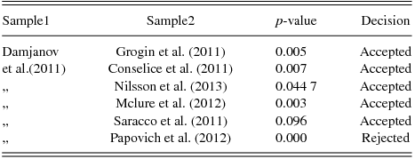
Since the data sets are chosen from different sources, they have various selection biases and errors, etc. Hence, to judge their compatibility we have performed a multivariate multi sample matching test (Puri & Sen Reference Puri and Sen1966; Mckean, Biedermann, & Büger Reference McKean, Biedermann and Büger1974; Mondal et al. Reference Mondal, Chattopadhyay and Chattopadhyay2008) to see whether they have the same parent distribution or not. From previous works, it is evident that galaxies have undergone cosmological evolution via merger or accretion (Khochfar & Silk 2006; De Lucia & Blaziot Reference De Lucia and Blaizot2007; Guo & White Reference Guo and White2008; Kormendy et al. Reference Kormendy2009; Hopkins, Carton, & Bundy Reference Hopkins, Carton and Bundy2010; Naab Reference Naab, Pasquali and Ferreras2013) and we have performed the matching test for galaxies within the same redshift zone. The data set taken from Damjanov et al. (Reference Damjanov, Abraham and Glazebrook2011) contains maximum number of galaxies within the entire redshift zone (0.2 ⩽ z ⩽ 2.7) used in the present analysis. For this we have compared it with the other sets. The results are given in Table 1. It is clear from Table 1 that all the tests are accepted except one (Papovich et al. Reference Papovich, Bassett and Lotz2012) where the matching redshift zone is very narrow. Since almost in 99% cases, the test is accepted we assume that the data set consisting of samples from different sources is more or less homogeneous with respect to mass–size plane.
Table 1. Multivariate multi sample test for the matching of parent distributions corresponding to data sets 4–8 (at 0.5% level of significance).
For testing completeness of the combined data sets 4–8, we have plotted the data points in the size–mass plane (viz. Figure 1). Then we have performed V / V
max test. This test was first used by Schmidt (Reference Schmidt, Blaauw and Schmidt1965) to study the space distribution of a complete sample of radio quasars from 3eR catalogue. According to the test, let Fm
be the limiting flux of a survey. We define two columns $ V ( r) = \frac{4 \pi r^3}{3}$
and
$ V ( r) = \frac{4 \pi r^3}{3}$
and $ V_{\text{max}} = \frac{4 \pi r_m^3}{3}$
, where r is the radial distance to a quasar and rm
is the limiting distance at which flux of a quasar with luminosity L reduces to rm
. For r > rm
the quasars do not belong to the sample under consideration. If the quasars are expected to be uniformly distributed then V / V
max are uniformly distributed over [0, 1]. Then 〈V / V
max〉 = 0.5. According to the above theory, we have computed 〈log Re
/log Re
,max〉 for the combined data set and it is ~ 0.3, i.e. the combined data set of high redshift galaxies is complete up to an accuracy of almost 70%. For comparison we have also plotted the combined data sets 1–3, in the size–mass plane (viz. Figure 2).
$ V_{\text{max}} = \frac{4 \pi r_m^3}{3}$
, where r is the radial distance to a quasar and rm
is the limiting distance at which flux of a quasar with luminosity L reduces to rm
. For r > rm
the quasars do not belong to the sample under consideration. If the quasars are expected to be uniformly distributed then V / V
max are uniformly distributed over [0, 1]. Then 〈V / V
max〉 = 0.5. According to the above theory, we have computed 〈log Re
/log Re
,max〉 for the combined data set and it is ~ 0.3, i.e. the combined data set of high redshift galaxies is complete up to an accuracy of almost 70%. For comparison we have also plotted the combined data sets 1–3, in the size–mass plane (viz. Figure 2).

Figure 1. log Re versus log M plot of the data points for data sets 4–8.

Figure 2. log Re versus log M plot of the data points for data sets 1–3.
It is to be noted that in Ho et al. (Reference Ho2011) paper, the magnitude values of the three components corresponding to each ETG are given from which, luminosities are computed. Then these luminosities are multiplied by (M/L) ratios for obtaining stellar masses. The (M/L) ratios are computed following Bell & de Zong (Reference Bell and de Zong2001). We have not been able to retrieve data for some high redshift galaxies and instead included some new data from other recent references so that sample size of high redshift galaxies are somewhat reduced in our case, but the overall distribution of these galaxies are similar in the size-redshift plane with those considered by Huang et al. (2013b) (viz. Figure 1 of Huang et al. (2013) and Figure 3 in the present work) except the region 1 ⩽ z ⩽ 2 which is more populated than Huang et al. (2013b) sample as we have included new galaxies in data sets 4–8.

Figure 3. Logarithm of the effective radius versus redshift plot for the entire sample of ETGs in 0.2 ⩽ z ⩽ 2.7.
3 METHOD
The theory of the special distribution of galaxies has been discussed by several authors like Peebles (Reference Peebles1980), Blake et al. (Reference Blake, Pope, Scott and Mobasher2006), Martinez & Saar (Reference Martinez and Saar2002), etc. During 1950s, the most extensive statistical study was performed by Neyman and Scott. Their work was based on the large amount of data obtained from the LICK survey. The main empirical statistics they used were the angular auto correlation function of the galaxy counts (Neyman, Scott, & Shane Reference Oser1956) and Zwicky’s index of clumpiness (Neyman, Scott, & Shane Reference Neyman, Scott and Shane1954).
Neyman & Scott (Reference Neyman and Scott1952) introduced this theory on the basis of four assumptions viz. (i) galaxies occur only in clusters, (ii) the number of galaxies varies from cluster to cluster subject to a probabilistic law, (iii) the distribution of galaxies within a cluster is also subject to a probabilistic law, and (iv) the distribution of cluster centres in space is subject to a probabilistic law described as quasi-uniform. As the observed distribution of number of galaxies does not follow Poisson law, it is suspected that not only the apparent but also the actual spatial distribution of galaxies is clustered.
In the present work, attempts have been made to establish the same postulates with respect to mass–size distribution of galaxies. Here the hypothesis is ‘there is clustering nature also in the galaxy distribution with respect to the parameters mass and size of the galaxies’. This particular hypothesis also has been studied by several authors. But we have followed the same approach as that used to establish spatial clustering as discussed above.
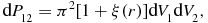
In cosmology the cross-correlation function ξ(r) of a homogeneous point process is defined by
 \begin{equation}
\text{d}P_{12}=\pi ^{2}[1+\xi (r)]\text{d}V_{1}\text{d}V_{2},
\end{equation}
\begin{equation}
\text{d}P_{12}=\pi ^{2}[1+\xi (r)]\text{d}V_{1}\text{d}V_{2},
\end{equation}
where r is the separation vector between the points x 1 and x 2 and π is mean number density. Considering two infinitesimally small spheres centred in x 1 and x 2 with volumes dV1 and dV2 , the joint probability that in each of the spheres lies a point of the point process is as follows:
 \begin{equation}
\text{d}P_{12}=\lambda _{2}(x_{1},x_{2})\text{d}V_{1}\text{d}V_{2}.
\end{equation}
\begin{equation}
\text{d}P_{12}=\lambda _{2}(x_{1},x_{2})\text{d}V_{1}\text{d}V_{2}.
\end{equation}
In (2), λ2(x 1, x 2) is defined as the second order intensity function of a point process.
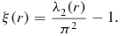
If the point field is homogeneous, the second-order intensity function λ2(x 1, x 2) depends only on the distance r = |x 1 − x 2| and direction of the line passing through x 1 and x 2. If, in addition, the process is isotropic,the direction is not relevant and the function only depends on r and may be denoted by λ2(r). Then
 \begin{equation}
\xi (r)=\frac{\lambda _{2}(r)}{\pi ^{2}}-1.
\end{equation}
\begin{equation}
\xi (r)=\frac{\lambda _{2}(r)}{\pi ^{2}}-1.
\end{equation}
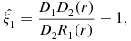
Different authors proposed several estimators of ξ(r). Natural estimators have been proposed by Peebles & Hauser (Reference Peebles and Hauser1974). The cross-correlation function ξ(r) can be estimated from the galaxy distribution by constructing pair counts from the data sets. A pair count between two galaxy populations 1 and 2, D 1 D 2(r), is a frequency corresponding to separation r to r+δr for a bin of width δr in the histogram of the distribution r, DiRj and RiRj denote the same pair counts corresponding to one galaxy sample and two simulated samples respectively, i, j = 1, 2. Two natural estimators are given by
 \begin{equation}
\hat{\xi _{1}} = \frac{D_{1}D_{2}(r)}{D_{2}R_{1}(r)}-1, \\
\end{equation}
\begin{equation}
\hat{\xi _{1}} = \frac{D_{1}D_{2}(r)}{D_{2}R_{1}(r)}-1, \\
\end{equation}
 \begin{equation}
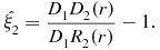
\hat{\xi _{2}} = \frac{D_{1}D_{2}(r)}{D_{1}R_{2}(r)}-1.
\end{equation}
\begin{equation}
\hat{\xi _{2}} = \frac{D_{1}D_{2}(r)}{D_{1}R_{2}(r)}-1.
\end{equation}
Another two improved estimators are Blake et al. (Reference Blake, Pope, Scott and Mobasher2006)
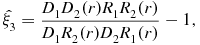 \begin{equation}
\hat{\xi _{3}}=\frac{D_{1}D_{2}(r)R_{1}R_{2}(r)}{D_{1}R_{2}(r) D_{2}R_{1}(r)}-1,
\end{equation}
\begin{equation}
\hat{\xi _{3}}=\frac{D_{1}D_{2}(r)R_{1}R_{2}(r)}{D_{1}R_{2}(r) D_{2}R_{1}(r)}-1,
\end{equation}
and
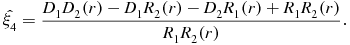 \begin{equation}
\hat{\xi _{4}}=\frac{D_{1}D_{2}(r)-D_{1}R_{2}(r)-D_{2}R_{1}(r)+R_{1}R_{2}(r)}{R_{1}R_{2}(r)}.
\end{equation}
\begin{equation}
\hat{\xi _{4}}=\frac{D_{1}D_{2}(r)-D_{1}R_{2}(r)-D_{2}R_{1}(r)+R_{1}R_{2}(r)}{R_{1}R_{2}(r)}.
\end{equation}
The first two estimates are potentially biased. As in the present situation, we are considering mass–size parametric space, we have taken r as the Euclidean distance between two (mass–size) points of two galaxies, either original or simulated. In order to generate simulated samples of mass and size, we have used uniform distribution of mass and size with ranges selected from original samples. Here, r is normalised by dividing the original separation by the maximum separation.
3.1. Simulation and computation
In order to determine the cross-correlation function by incorporating the effects of the statistical fluctuations, we have generated random unclustered realisations (denoted by Ri ) of the mass–size distribution in the same range as that of the corresponding observed samples (denoted by Di ).
The simulation and computation steps are as follows:
-
(i) Select one pair of observed bivariate (mass–size) samples. These are denoted by D 1 and D 2.
-
(ii) Corresponding to D 1, determine the minimum and maximum values of masses and sizes, respectively. Let the values be (m min, m max) and (s min, s max), respectively.
-
(iii) Assuming uniform distribution of masses over the range m min < m < m max, generate one mass at random. Let it be m 1. Similarly assuming uniform distribution over the range s min < s < s max, generate one size at random. Let it be s 1. Then (m 1, s 1) will give the first paired observation for the simulated sample R 1.
-
(iv) Repeat step (iii), a large number of times in order to generate a large number of paired values for the simulated sample R 1.
-
(v) Repeat the steps (ii)–(iv) for D 2 in order to generate R 2.
-
(vi) After computing the Euclidean distances between pairs (DiRj ), i, j = 1, 2 and construction of histograms, compute the cross-correlation function by using formulae (6) and (7) in order to find estimator 1 and estimator 2.
-
(vii) Repeat steps (i)–(iv) by considering different pairs of (mass–size) samples.
-
(viii) To compute the standard errors of estimators use boot strap method.
4 RESULTS AND DISCUSSION
We have computed the cross-correlation functions of each of data sets 1–3 with data sets 4–8, i.e. we have tried to find any kind of correlation between three components of nearby ETGs with high redshift ETGs in five redshift bins as mentioned above. We have found significant correlation between data sets 1 and 8 and between data sets 2 and 4. This is clear from Figures 4 and 5, respectively where the correlations are as high as 0.5 ± (0.02–0.07) and 0.65 ± (0.03–0.07) for both the estimates at minimum separation (viz.r ~ 0.1). These show that the innermost components of nearby elliptical galaxies are well in accordance with highest redshift massive ETGs (viz. mass ~ 1011.14 M⊙ and R e ~ 0.92 kpc), known as ‘red nuggets’ but the intermediate components are highly correlated with galaxies in the redshift bin 0.5 ⩽ z ⩽ 0.75 having median mass and size, 1010.87 M⊙ and 2.34 kpc, respectively. If we merge data sets 1 and 2 and compare with high z galaxies in five redshift bins, the cross-correlation functions are all close to zero at all separations unlike Huang et al. (2013b).

Figure 4. Cross-correlation function ξ(r) versus normalised distance bin r between data sets 1 and 8. The solid lines are power laws for both the estimators as $\xi (r) \propto \frac{1}{r}.$

Figure 5. Cross-correlation function ξ(r) versus normalised distance bin r between data sets 2 and 4. The solid lines are power law fits for both the estimators as $\xi (r) \propto \frac{1}{r}$
.
$\xi (r) \propto \frac{1}{r}$
.
The above result is somewhat consistent with the work of Huang et al. (2013b) in a sense that the inner and intermediate parts are the fossil evidences of high redshift galaxies but unlike Huang et al. (2013b), components 1 and 2 together show no correlation with all high redshift ETGs together and they are highly correlated with high redshift ETGs in two redshift bins. This indicates clearly two different epochs of structure formation as shown by their z values.
After finding the cross-correlation functions between data sets 1 and 8, we have fitted a power law assuming the relation
 \begin{equation}
\xi (r) \propto \frac{1}{r},
\end{equation}
\begin{equation}
\xi (r) \propto \frac{1}{r},
\end{equation}
i.e.
 \begin{equation}
\xi (r) = A r^{-1},
\end{equation}
\begin{equation}
\xi (r) = A r^{-1},
\end{equation}
where for estimator 1, A = 0.026 72 and for estimator 2, A = 0.031 395.
We have also performed Kolmogorov–Smirnov test (Kolmogorov Reference Kolmogorov1933) for justifying the goodness of fit of the power law. Here fitting of power law helps us to reject a model with no correlation and the KS test indicates the significance level (p-value) which is quite high in the present situation. Here, we have assumed that the cross correlations and the fitted values are samples coming from the distribution function of a Pareto distribution. The p-values for this test for estimator 1 is 0.417 5 and for estimator 2 is 0.786 9, signifying that the tests are accepted and the fitted power law gives well justification for the cross-correlation and distance relationship. We have fitted similar power laws for cross-correlation function and distance for data sets 2 and 4. Here, the proportionality constants are 0.024 7 for estimator 1 and 0.036 9 for estimator 2. The Kolmogorov–Smirnov tests give p-values = 0.786 9 for both the estimators, signifying that in this case also the relationship is well justified.
On the other hand, cross-correlation function, computed for data set 3 with galaxies in the above five bins are all insignificant which is clear from Figure 6.

Figure 6. Cross-correlation function ξ(r) versus normalised distance bin r between data set 3 and all redshift bins.
It is well known that major and minor mergers take important role in the formation and evolution of massive elliptical galaxies (Khochfar & Silk 2006; De Lucia & Blaizot Reference De Lucia and Blaizot2007; Guo & White Reference Guo and White2008; Kormendy et al. Reference Kormendy2009; Hopkins et al. Reference Hopkins, Carton and Bundy2010; Naab Reference Naab, Pasquali and Ferreras2013). Generally ellipticals having maximum masses are speculated to be formed at z ~ 6 or higher and the environment for their formation is a dissipative one. Subsequently, they become massive (~1011 M⊙) and compact in a very short interval of time at z ~ 2 (Dekel et al. Reference Dekel, Sari and Ceverino2009; Oser et al. Reference Oser2010; Feldmann, Carollo, & Mayer Reference Feldmann, Carollo and Mayer2011; Oser et al. Reference Oser2012). But at the same time a significant fraction remains less active at z ~ 2. They are 4–5 times more compact and less massive by a factor of 2 corresponding to their low-redshift descendants (Buitrago et al. 2008; van Dokkum et al. 2008; VanderWel et al. 2008; Cimatti, Cassata, & Pozzetti Reference Cimatti, Cassata and Pozzetti2008; Bezanson et al. Reference Bezanson2009; van Dokkum et al. Reference van Dokkum, Whitaker and Brammer2010; Whitaker et al. Reference Whitaker2012).
For the massive ellipticals in the present sample, the innermost cores (data set 1) are well in accordance with highest redshift (2.0 < z ⩽ 2.7) galaxies and their core masses (viz. median value ~1010.203 M⊙ and 1010.6839 M⊙, respectively). Hence, it is reasonable to separate that these high redshift population forms the cores of at least some, if not all, present day massive ellipticals. Thus formation of massive ellipticals only by monolithic collapse model is challenged because they will be too small and too red (van Dokkum et al. 2008; Ferré-Mateu, Vazdekis, & Trujillo Reference Ferré-Mateu, Vazdekis and Trujillo2012), the subsequent evolution forming the intermediate (data set 2) and outer part (data set 3) might be as follows. On the aspect of major or minor major, following Naab, Johansson, & Ostriker (Reference Naab, Johansson and Ostriker2009) it is seen that if Mi and ri be the mass and radius of a compact initial stellar system with a total energy Ei and mean square speed ⟨v 2 i ⟩ and Ma, ra, Ea and ⟨v 2 a ⟩ be the corresponding values after merger with other systems then,
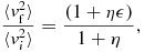 \begin{equation}
\frac{\langle v^{2}_{\rm f}\rangle }{\langle v^{2}_{i}\rangle } = \frac{(1+\eta \epsilon )}{1+\eta } , \\
\end{equation}
\begin{equation}
\frac{\langle v^{2}_{\rm f}\rangle }{\langle v^{2}_{i}\rangle } = \frac{(1+\eta \epsilon )}{1+\eta } , \\
\end{equation}
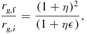 \begin{equation}
\frac{r_{g,{\rm f}}}{r_{g,i}} = \frac{(1+\eta )^{2}}{(1+\eta \epsilon )} , \\
\end{equation}
\begin{equation}
\frac{r_{g,{\rm f}}}{r_{g,i}} = \frac{(1+\eta )^{2}}{(1+\eta \epsilon )} , \\
\end{equation}
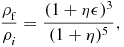 \begin{equation}
\frac{\rho _{\rm f}}{\rho _{i}} = \frac{(1+\eta \epsilon )^{3}}{(1+\eta )^{5}} ,
\end{equation}
\begin{equation}
\frac{\rho _{\rm f}}{\rho _{i}} = \frac{(1+\eta \epsilon )^{3}}{(1+\eta )^{5}} ,
\end{equation} $\eta =\frac{M_{a}}{M_{i}}$
, ε = ⟨v
2
a
⟩/⟨v
2
i
⟩, ρ is the density. Then for η = 1 (major merger), the mean square speed remains same, the size increases by a factor of 2 and densities drop by a factor of 4. Now, in the present situation, the intermediate part (data set 2) has radii (median value ⟨R
e⟩2 ~ 2.560 kpc) which is almost 3 times larger than the radii of inner part (⟨R
e⟩ ~ 0.6850 kpc).
$\eta =\frac{M_{a}}{M_{i}}$
, ε = ⟨v
2
a
⟩/⟨v
2
i
⟩, ρ is the density. Then for η = 1 (major merger), the mean square speed remains same, the size increases by a factor of 2 and densities drop by a factor of 4. Now, in the present situation, the intermediate part (data set 2) has radii (median value ⟨R
e⟩2 ~ 2.560 kpc) which is almost 3 times larger than the radii of inner part (⟨R
e⟩ ~ 0.6850 kpc).
Also in a previous work (Chattopadhyay et al. Reference Chattopadhyay2009; Chattopadhyay, Mondal, & Chattopadhyay Reference Chattopadhyay, Mondal and Chattopadhyay2013) on the brightest elliptical galaxy NGC 5128, we have found three groups of globular clusters. One is originated in original cluster formation event that coincided with the formation of elliptical galaxy and the other two, one from accreted spiral galaxy and other from tidally stripped dwarf galaxies. Hence we may conclude from the above discussion that the intermediate parts of massive elliptical is formed via major merger with the high redshift galaxies in 0.5 ⩽ z < 0.75, whose median mass and size are respectively 1010.87 M⊙ & 2.34 kpc, respectively.
In the limit when ⟨v 2 a ⟩ ≪ ⟨v 2 i ⟩ or ε ≪ 1, the size increases by a factor of 4 (minor merger). In the present case, the outermost parts of massive ellipticals have sizes much larger (⟨R e⟩3 ~ 10.54 kpc), so ⟨R e⟩3 − ⟨R e⟩1 ~ 10 kpc) than innermost part. Also, median mass of this part is of the order of 1010.6839 M⊙ which is comparable to the combined masses of few dwarf galaxies. So, it might be suspected that the outermost part is primarily composed of stellar components of tidally accreted satellite dwarf galaxies. This is also consistent with our previous works (Chattopadhyay et al. Reference Chattopadhyay2009, Reference Chattopadhyay, Mondal and Chattopadhyay2013) in case of NGC 5128. Since, data set 3 has no correlations with any subset of high redshift galaxies, we cannot specifically confirm their formation epoch but we can atmost say that their formation process is different from the innermost and intermediate part.
Finally, we can conclude that formation of nearby massive ellipticals have three parts, inner, intermediate, and outermost, whose formation mechanisms are different. The innermost parts are descendants of high ETGs called ‘red nuggets’. The innermost parts are formed by major mergers with tidally stripped satellite dwarf galaxies (Mondal et al. Reference Mondal, Chattopadhyay and Chattopadhyay2008; Chattopadhyay et al. Reference Chattopadhyay2009, Reference Chattopadhyay, Mondal and Chattopadhyay2013; Mihos et al. Reference Mihos2013). Since, the densities and velocity dispersion values and abundances are not available with the present data sets, so more specific conclusions can be drawn if these data are available for massive ellipticals and satellite dwarfs. But at this moment we can say, that since two different formation scenarios are very unlikely for the same galaxy at a particular epoch, so the above study is indicative of a ‘third phase’ of formation of the outermost parts of massive nearby ellipticals rather than a ‘two phase one’ as indicated by previous authors.
ACKNOWLEDGEMENTS
The authors are grateful to the referee for suggestions in improving the quality of the work.


