3.1 Recombination radiation: The origin of the factor ‘0.68’

The volume Lyα emissivity following recombination is often given by

(3) \begin{equation} j_{{\rm rec}}(n,T\,\nu )=0.68 n_{\rm e} n_{\rm p} \alpha _{\rm B}(T)\phi (\nu )E_{\alpha }/(\sqrt{\pi }\Delta \nu _{\rm D}), \end{equation}

where E _α = 10.2 eV, n _e/n _p denotes the number density of free electrons/protons, and ϕ(ν) denotes the Voigt profile (normalised to $\int d\nu \hspace{2.84526pt}\phi (\nu )=\sqrt{\pi }\Delta \nu _{\rm D}$ , in which $\Delta \nu _{\rm D}=1.1\times 10^{11}(T/10^4\hspace{2.84526pt}{\rm K})^{1/2}$ Hz quantifies thermal broadening of the line). Expressions for ϕ(ν) are given in Section 4.1. The factor 0.68 denotes the fraction of recombination events resulting in Lyα and is derived next.

The capture of an electron by a proton generally results in a hydrogen atom in an excited state (n, l). Once an atom is in a quantum state (n, l) it radiatively cascades to the ground state n = 1, l = 0 via intermediate states (n_i, l_i ). The probability that a radiative cascade from the state (n, l) results in a Lyα photon is given by

(4) \begin{eqnarray} P(n,l\rightarrow {\rm Ly}\alpha )&=& \sum _{n^{\prime },l^{\prime }}P(n,l\rightarrow n^{\prime },l^{\prime })P(n^{\prime },l^{\prime }\rightarrow {\rm Ly}\alpha ). \end{eqnarray}

That is, the probability can be computed if one knows the probability that a radiative cascade from lower excitation states (n′, l′) results in the emission of a Lyα photon, and the probabilities that the atom cascades into these lower excitation states, P(n, l → n′, l′). This latter probability is given by

(5) \begin{equation} P(n,l\rightarrow n^{\prime },l^{\prime })=\frac{A_{n,l,n^{\prime },l^{\prime }}}{\sum _{n^{\prime \prime },l^{\prime \prime }}A_{n,l,n^{\prime \prime },l^{\prime \prime }}}, \end{equation}

in which A _{n, l, n′, l′} denotes the Einstein A-coefficient for the nl → n′l′ transitionFootnote ³ .

The quantum mechanical selection rules only permit transitions for which |l − l′| = 1, which restricts the total number of allowed radiative cascades. Figure 1 schematically depicts permitted radiative cascades in a four-level H atom. Green solid lines depict radiative cascades that result in a Lyα photon, while red dotted lines depict radiative cascades that do not yield a Lyα photon.

Figure 1. This Figure shows a schematic diagram of the energy levels of a hydrogen atom. The energy of a quantum state increases from bottom to top. Each state is characterised by two quantum numbers n (principle quantum number) and l (orbital quantum number). Recombination can put the atom in any state nl, which then undergoes a radiative cascade to the groundstate (1S). Quantum selection rules dictate that the only permitted transitions have Δl = ±1. These transitions are indicated in the Figure. Green lines [red dotted lines] show cascades that [do not] result in Lyα. The lower right panel shows that probability that a cascade from state nl results in Lyα, P(n, l → Lyα) (Equation (5)).

Figure 1 also contains a table that shows the probability P(n′, l′ → Lyα) for n ⩽ 5. For example, the probability that a a radiative cascade from the (n, l) = (3, 1) state (i.e. the 3p state) produces a Lyα photon is 0, because the selection rules only permit the transitions (3, 1) → (2, 0) and (3, 1) → (1, 0). The first transition leaves the H-atom in the 2 s state, from which it can only transition to the ground state by emitting two photons (Breit & Teller Reference Breit and Teller1940). On the other hand, a radiative cascade from the (n, l) = (3, 2) state (i.e. the 3d state) will certainly produce a Lyα photon, since the only permitted cascade is $(3,2)\rightarrow (2,1)\overset{{\rm Ly}\alpha }{\rightarrow }(1,0)$ . Similarly, the only permitted cascade from the 3s state is $(3,0)\rightarrow (2,1)\overset{{\rm Ly}\alpha }{\rightarrow }(1,0)$ , and P(3, 0 → Lyα) = 1. For n > 3, multiple radiative cascades down to the ground state are generally possible, and P(n, l → Lyα) takes on values other than 0 or 1 (see e.g. Spitzer & Greenstein Reference Spitzer and Greenstein1951).

The probability that an arbitrary recombination event results in a Lyα photon is given by

(8) \begin{equation} P({\rm Ly}\alpha )= \sum _{n_{\rm min}}^{\infty } \sum _{l=0}^{n-1}\frac{\alpha _{nl}(T)}{\alpha _{\rm tot}(T)}P(n,l\rightarrow {\rm Ly}\alpha )\, \end{equation}

where the first term denotes the fraction of recombination events into the (n, l) state, in which α_tot denotes the total recombination coefficient α_tot(T) = ∑^∞ _{n min} ∑ ^{n − 1} _{l = 0}α _nl (T). The temperature-dependent state specific recombination coefficients α _nl (T) can be found in for example (Burgess Reference Burgess1965) and Rubiño-Martín, Chluba, & Sunyaev (Reference Rubiño-Martín, Chluba and Sunyaev2006). The value of n _min depends on the physical conditions of the medium in which recombination takes place, and two cases bracket the range of scenarios commonly encountered in astrophysical plasmas:

• • ‘case-A’ recombination: recombination takes place in a medium that is optically thin at all photon frequencies. In this case, direct recombination to the ground state is allowed and n _min = 1.

• • ‘case-B’ recombination: recombination takes place in a medium that is opaque to all Lyman seriesFootnote ⁴ photons (i.e. Lyα, Lyβ, Lyγ, . . .), and to ionising photons that were emitted following direct recombination into the ground state. In the so-called ‘on the spot approximation’, direct recombination to the ground state produces an ionising photon that is immediately absorbed by a nearby neutral H atom. Similarly, any Lyman series photon is immediately absorbed by a neighbouring H atom. This case is quantitatively described by setting n _min = 2, and by setting the Einstein coefficient for all Lyman series transitions to zero, i.e. A _{np, 1s} = 0.

Figure 2 shows the total probability P(Lyα) (Equation (8)) that a Lyα photon is emitted per recombination event as a function of gas temperature T, assuming case-A recombination (solid line), and case-B recombination (dashed line). For gas at T = 10⁴ K and case-B recombination, we have P(Lyα) = 0.68. This value ‘0.68′ is often encountered during discussions on Lyα emitting galaxies. It is worth keeping in mind that the probability P(Lyα) increases with decreasing gas temperature and can be as high as P(Lyα) = 0.77 for T = 10³ K (also see Cantalupo, Porciani, & Lilly Reference Cantalupo, Porciani and Lilly2008). The red open circles represent the following two fitting formulae

(9) \begin{eqnarray} P_{\rm A}({\rm Ly}\alpha )\eqcellsep=\eqcellsep 0.41-0.165 \log T_4-0.015(T_4)^{-0.44}\\ \nonumber P_{\rm B}({\rm Ly}\alpha )\eqcellsep=\eqcellsep 0.686-0.106 \log T_4-0.009(T_4)^{-0.44}, \end{eqnarray}

where T ₄ ≡ T/10⁴ K. The fitting formula for case-B is taken from Cantalupo et al. (Reference Cantalupo, Porciani and Lilly2008).

Figure 2. The top panel shows the number of Lyα photons per recombination event, P(Lyα), as a function of temperature for case-A (solid line) and case-B (dashed line). In both cases, P(Lyα) decreases with temperature. For comparison, the filled circle at [T, P _B(Lyα)] = [10⁴, 0.68] is the number that is given by Osterbrock (Reference Osterbrock1989) and which is commonly used in the literature (other values given in Osterbrock 1989 are shown as filled circles). The top panel shows for example that at T = 0.5 × 10⁴ K (T = 2 × 10⁴ K), P _B(Lyα) = 0.70 (P _B(Lyα) = 0.64). A stronger temperature dependence is found for case-A recombination. The bottom panel shows the total case-A and case-B recombination coefficients. The recombination coefficient α _B decreases more rapidly with temperature than α _A , which implies that the fractional contribution from direct recombination into the ground state increases with temperature. Generally, as temperature increases a larger fraction of recombination events goes into the other low − n states which reduces the number of Lyα photons per recombination event. Red open circles represent fitting formulae given in Equation (9).

Recombinations in HII regions in the ISM are balanced by photoionisation in equilibrium HII regions. The total recombination rate in an equilibrium HII region therefore equals the total photoionisation rate, or the total rate at which ionising photons are absorbed in the HII region (in an expanding HII region, the total recombination rate is less than the total rate at which ionising photons are absorbed). If a fraction f ^ion _esc of ionising photons is not absorbed in the HII region (and hence escapes), then the total Lyα production rate in recombinations can be written as

(10) \begin{eqnarray} \dot{N}^{\rm rec}_{{\rm Ly}\alpha }\eqcellsep=\eqcellsep P({\rm Ly}\alpha )(1-f_{\rm esc})\dot{N}_{\rm ion} \\ \nonumber \eqcellsep\eqcellsep\approx 0.68(1-f^{\rm ion}_{\rm esc})\dot{N}_{\rm ion},\hspace{2.84526pt}\hspace{2.84526pt}{\rm {\it case}}-B,\hspace{2.84526pt}{\rm T}=10^4\hspace{2.84526pt}{\rm K} \end{eqnarray}

where $\dot{N}_{\rm ion}$ ( $\dot{N}^{\rm rec}_{{\rm Ly}\alpha }$ ) denotes the rate at which ionising (Lyα recombination) photons are emitted. The equation on the second line is commonly adopted in the literature. The ionising emissivity of star-forming galaxies is expected to be boosted during the EoR: stellar evolution models combined with stellar atmosphere models show that the effective temperature of stars of fixed mass become hotter with decreasing gas metallicity (Tumlinson & Shull Reference Tumlinson and Shull2000; Schaerer Reference Schaerer2002). The increased effective temperature of stars causes a larger fraction of their bolometric luminosity to be emitted as ionising radiation. We therefore expect galaxies that formed stars from metal poor (or even metal free) gas during the EoR, to be strong sources of nebular emission. Schaerer (Reference Schaerer2003) provides the following fitting formula for $\dot{N}_{\rm ion}$ as a function of absolute gas metallicityFootnote ⁵ Z _gas, $\log \dot{N}_{\rm ion}=-0.0029\times (\log Z_{\rm gas} +9.0)+53.81$ , which is valid for a Salpeter IMF in the mass range M = 1 − 100M _⊙.

A useful measure for the ‘strength’ of the Lyα line (other than just its flux) is given by the equivalent width

(11) \begin{equation} {\rm EW}\equiv \int d \lambda \hspace{2.84526pt}(F(\lambda ) - F_0)/F_0, \end{equation}

which measures the total line flux compared to the continuum flux density just redward (as the blue side can be affected by intergalactic scattering, see Section 5.2) of the Lyα line, F ₀. For ‘regular’ star-forming galaxies (Salpeter IMF, solar metallicity) the maximum physically allowed restframe EW is EW_max ~ 240 Å (see e.g. Schaerer Reference Schaerer2003; Laursen, Duval, & Ostlin Reference Laursen, Duval and Ostlin2013, and references therein). Reducing the gas metallicity by as much as two orders of magnitude typically boosts the EW_max, but only by ≲50% (Laursen et al. Reference Laursen, Duval and Ostlin2013). A useful way to gain intuition on EW is that EW ~ FWHM × (relative peak flux density). That is, for typical observed (restframe) FWHM of Lyα lines of FWHM ~ 1 − 2 Å, EW=240 Å corresponds to having a relative flux density in the peak of the line that is ~ 100 times that in the continuum.

3.2 Collisionally-excited (a.k.a ‘cooling’) radiation

Lyα photons can also be produced following collisional-excitation of the 2p transition when a hydrogen atoms deflects the trajectory of an electron that is passing by. The Lyα emissivity following collisional-excitation is given by

(12) \begin{equation} j_{{\rm coll}}(n,T,\nu )=\phi (\nu )n_{\rm e} n_{\rm HI}q_{\rm 1s2p} E_{\alpha }/(\sqrt{\pi }\Delta \nu _{\rm D}), \end{equation}

where n _HI denotes the number density of hydrogen atoms and

(13) \begin{equation} q_{1s2p}(T)=8.63\times 10^{-6}T^{-1/2}\langle \Omega _{1s2p}\rangle \exp \Big {(} -\frac{E_{\alpha }}{k_BT}\Big {)}\hspace{2.84526pt}{\rm cm}^{3\hspace{2.84526pt}}{\rm s}^{-1} \end{equation}

where ⟨Ω_1s2p ⟩(T) denotes the velocity averaged collision strength, which depends weakly on temperature. The top panel of Figure 3 shows the temperature dependence of ⟨Ω _lu ⟩ for the 1s → 2s (dotted line), 1s → 2p (dashed line), and for their sum 1s → 2 (black solid line) as given by Scholz et al. (Reference Scholz, Walters, Burke and Scott1990); Scholz & Walters (Reference Scholz and Walters1991). Also shown are velocity averaged collision strengths for the 1s → 3 (red solid line, obtained by summing over all transitions 3s, 3p and 3d), and 1s → 4 (blue solid line, obtained by summing over all transitions 4s, 4p, 4d and 4f) as given by Aggarwal et al. (Reference Aggarwal, Berrington, Burke, Kingston and Pathak1991). The bottom panel shows the collision coupling parameter q _lu for the same transitions. This plot shows that collisional coupling to the n = 2 level increases by ~ 3 orders of magnitude magnitude when T = 10⁴ K → T = 2 × 10⁴ K. The actual production rate of Lyα photons can be even more sensitive to T, as both n _e sharply increases with T and n _HI sharply decreases with T within the same temperature range (under the assumption that collisional ionisation balances recombination, which is relevant in e.g self-shielded gas, see e.g. Figure 1 in Thoul & Weinberg Reference Thoul and Weinberg1995).

Figure 3. Top panel: velocity averaged collision strength ⟨Ω _lu ⟩ as a function of temperature T for the Lyα (1s → 2p) transition (black dashed line). The black dotted line corresponds to the 1s → 2s transitions. Solid lines indicate transitions from the ground-state to excited states (summed over different orbital quantum numbers). Bottom panel: collision coupling q _lu (Equation (13)) for the same transitions.

This process converts thermal energy of the gas into radiation, and therefore cools the gas. Lyα cooling radiation has been predicted to give rise to spatially extended Lyα radiation (Haiman, Spaans, & Quataert Reference Haiman, Spaans and Quataert2000; Fardal et al. Reference Fardal, Katz and Gardner2001), and provides a possible explanation for Lyα ‘blobs’ (Dijkstra & Loeb Reference Dijkstra and Loeb2009; Goerdt et al. Reference Goerdt, Dekel and Sternberg2010; Faucher-Giguère et al. Reference Faucher-Giguère, Kereš, Dijkstra, Hernquist and Zaldarriaga2010; Rosdahl & Blaizot Reference Rosdahl and Blaizot2012). In these models, the Lyα cooling balances ‘gravitational heating’ in which gravitational binding energy is converted into thermal energy in the gas.

Precisely how gravitational heating works is poorly understood. Haiman et al. (Reference Haiman, Spaans and Quataert2000) propose that the gas releases its binding energy in a series of ‘weak’ shocks as the gas navigates down the gravitational potential well. These weak shocks convert binding energy into thermal energy over a spatially extended region, which is then reradiated primarily as Lyα. It is possible that a significant fraction of the gravitational binding energy is released very close to the galaxy (e.g. when gas free-falls down into the gravitational potential well, until it is shock heated when it ‘hits’ the galaxy Birnboim & Dekel Reference Birnboim and Dekel2003). It has been argued that some compact Lyα emitting sources may be powered by cooling radiation (as in Birnboim & Dekel Reference Birnboim and Dekel2003; Dijkstra Reference Dijkstra2009; Dayal, Ferrara, & Saro Reference Dayal, Ferrara and Saro2010). Recent hydrodynamical simulations of galaxies indicate that the fraction of Lyα flux coming from galaxies in the form of cooling radiation increases with redshift, and may be as high as ~ 50% at z ~ 6 (Dayal et al. Reference Dayal, Ferrara and Saro2010; Yajima et al. Reference Yajima, Li and Zhu2012). However, one should take these numbers with caution, because the predicted Lyα cooling luminosity depends sensitively on the gas temperature of the ‘cold’ gas (i.e. around T ~ 10⁴ K, as illustrated by the discussion above). It is very difficult to reliably predict the temperature of this gas, because the gas’ short cooling time drives the gas temperature to a value where its total cooling rate balances its heating rate. Because of this thermal equilibrium, we must accurately know and compute all the heating rates in the ISM (Faucher-Giguère et al. Reference Faucher-Giguère, Kereš, Dijkstra, Hernquist and Zaldarriaga2010; Cantalupo, Lilly, & Haehnelt Reference Cantalupo, Lilly and Haehnelt2012; Rosdahl & Blaizot Reference Rosdahl and Blaizot2012) to make a robust prediction for the Lyα cooling rate. These heating rates include for example photoionisation heating, which requires coupled radiation-hydrodynamical simulations (as Rosdahl & Blaizot Reference Rosdahl and Blaizot2012), or shock heating by supernova ejecta (e.g. Shull & McKee Reference Shull and McKee1979).

It may be possible to observationally constrain the contribution of cooling radiation to the Lyα luminosity of a source, through measurements of the Lyα equivalent width: the larger the contribution from cooling radiation, the larger the EW. Lyα emission powered by regular star-formation can have EW_max ~ 300 − 400 Å(see discussion above). Naturally, observations of Lyα emitting galaxies whose EW significantly exceeds EW_max (as in e.g. Kashikawa et al. Reference Kashikawa, Nagao and Toshikawa2012), may provide hints that we are detecting a significant contribution from cooling. However, the same signature can be attributed population III stars (e.g. Raiter et al. Reference Raiter, Schaerer and Fosbury2010), and/or galaxies forming stars with a top-heavy initial mass function (IMF, e.g. Malhotra & Rhoads Reference Malhotra and Rhoads2002), or stochastic sampling of the IMF (Forero-Romero & Dijkstra Reference Forero-Romero and Dijkstra2013). In theory one can distinguish cooling radiation from these other processes via the Balmer lines, because Lyα cooling radiation is accompanied by an Hα luminosity that is $\frac{j_{{\rm coll,Ly}\alpha }}{j_{{\rm coll,H}\alpha }}=\frac{E_{\alpha }}{E_{{\rm H}\alpha }}\frac{\langle \Omega _{\rm 1s2p}\rangle }{\langle \Omega _{\rm 13}\rangle }$ $\exp {(}\frac{E_{{\rm H}\alpha }}{k_{\rm B} T} {)}$ ~ 100 times weaker, which is much weaker than expected for case-B recombination (where the Hα flux is ~ 8 times weaker, e.g. Dijkstra & Loeb Reference Dijkstra and Loeb2009). Measuring the flux in the Hα line at these levels requires an IR spectrograph with a sensitivity comparable to that of JWSTFootnote ⁶ .

3.3 Boosting recombination radiation

Equation 10 was derived assuming case-B recombination. However, at $Z \lsim 0.03 Z_{\odot }$ significant departures from case-B are expected. These departures increase the Lyα luminosity relative to case-B (e.g. Raiter et al. Reference Raiter, Schaerer and Fosbury2010). This increase of the Lyα luminosity towards lower metallicities is due to two effects: (i) the increased temperature of the HII region as a result of a suppressed radiative cooling efficiency of metal-poor gas. The enhanced temperature in turn increases the importance of collisional processes. For example, collisional-excitation increases the population of H-atoms in the n = 2 state, which can be photoionised by lower energy photons. Moreover, collisional processes can mix the populations of atoms in their 2s and 2p states; (ii) harder ionising spectra emitted by metal poor(er) stars. Higher energy photons can in principle ionise more than 1 H-atom, which can boost the overall Lyα production per ionising photon. Raiter et al. (Reference Raiter, Schaerer and Fosbury2010) provide a simple analytic formula which capture all these effects:

(14) \begin{equation} \dot{N}^{\rm rec}_{{\rm Ly}\alpha }= f_{\rm coll} P(1-f^{\rm ion}_{\rm esc})\dot{N}_{\rm ion}, \end{equation}

where $P\equiv \langle E_{\gamma ,{\rm ion}} \rangle /13.6\hspace{2.84526pt}{\rm eV}$ , in which ⟨E _{γ, ion}⟩ denotes the mean energy of ionising photonsFootnote ⁷ . Furthermore, $f_{\rm coll}\equiv \frac{1+an_{\rm HI}}{b+cn_{\rm HI}}$ , in which a = 1.62 × 10^{− 3}, b = 1.56, c = 1.78 × 10^{− 3}, and n _HI denotes the number of density of hydrogen nuclei. Eq 14 resembles the ‘standard’ equation, but replaces the factor 0.68 with Pf _coll, which can exceed unity. Eq 14 implies that for a fixed IMF, the Lyα luminosity may be boosted by a factor of a few. Incredibly, for certain IMFs the Lyα line may contain 40% of the total bolometric luminosity of a galaxy, which corresponds to a rest frame EW ~ 4000 Å.

We point out that the collisional processes discussed here are distinct from the collisional-excitation process discussed above (in Section 3.2), as they do not directly produce Lyα photons. Instead, they boost the number of Lyα photons that we can produce per ionising photon.

4.1 The cross section

The frequency dependence of the Lyα absorption cross-section, σ_α(x), is described well by a Voigt function. That is

(15) \begin{eqnarray} \sigma _{\alpha }(x)\eqcellsep=\eqcellsep\sigma _0\times \frac{a_{\rm v}}{\pi } \int _{-\infty }^{+\infty }dy \frac{\exp (-y^2)}{(x-y)^2+a_{\rm v}^2}\equiv \sigma _0\times \phi (x).\\ \nonumber \sigma _0\eqcellsep=\eqcellsep \frac{f_{\alpha }}{\sqrt{\pi }\Delta \nu _{\rm D}}\frac{\pi e^2}{m_e c}=5.88 \times 10^{-14}(T/10^4\hspace{2.84526pt}{\rm K})^{-1/2}\hspace{2.84526pt}{\rm cm}^{2} \end{eqnarray}

where f _α = 0.416 denotes the Lyα oscillator strength, and $a_{\rm v}=A_{\alpha }/[4\pi \Delta \nu _{\rm D}]=4.7 \times 10^{-4}(T/10^{4}\hspace{2.84526pt}{\rm K})^{-1/2}$ denotes the Voigt parameter, and σ₀ denotes the cross section at line centre. We introduced the Voigt functionFootnote ⁸ ϕ(x), which is plotted as the black solid line in the upper panel of Figure 4. This Figure also shows that the Voigt function ϕ(x) is approximated accurately as

(16) \begin{eqnarray} \phi (x)\approx \left\lbrace \begin{array}{ll}\ e^{-x^2}& \mbox{`core', i.e.}\hspace{2.84526pt}|x|<x_{\rm crit};\\ \ \frac{a_{\rm v}}{\sqrt{\pi }x^2}& \mbox{`wing', i.e.}\hspace{2.84526pt}|x|>x_{\rm crit},\end{array} \right. \end{eqnarray}

where the transition from the Gaussian core (red dashed line) to the Lorentzian wing (blue dotted line)Footnote ⁹ occurs at x _crit ~ 3.2 at the gas temperature of T = 10⁴ K that we adopted. An even more accurate fit - which works well even in the regime where we transition from core to wing - is given in Tasitsiomi (Reference Tasitsiomi2006).

Figure 4. The black solid line in top panel shows the Lyα absorption cross section, σ_α(x), at a gas temperature of T = 10⁴ K as given by the Voigt function (Equation (15)). This Figure shows that the absorption cross section is described accurately by a Gaussian profile (red dashed line) in the ‘core’ at |x| < x _crit ~ 3.2 (or |Δv| < 40 km s^{− 1}), and by a Lorentzian profile in the ‘wing’ of the line (blue dotted line). The Voigt profile is only an approximate description of the real absorption profile. Another approximation includes the ‘Rayleigh’ approximation (grey solid line, see text). The green dotted line shows the absorption profile resulting from a full quantum mechanical calculation (Lee Reference Lee2013). The different cross sections are compared in the lower panel, which highlights that the main differences arise only far in the wings of the line.

It is important to point out that the Voigt function itself (as given by Equation (15)) only represents an approximation to the real frequency dependence of the absorption cross section. The Voigt profile is derived through a convolution of a Gaussian profile (describing the thermal velocity-distribution of HI atoms) with the Lorentzian profile (see above). A common modification of the Lorentzian is given in e.g. Peebles (Reference Peebles and Peebles1993, Reference Peebles1969), where the absorption cross section for a single atom includes an additional (ν/ν_α)⁴-dependence, as is appropriate for Rayleigh scatteringFootnote ¹⁰ . In this approximation we have (also see Schroeder et al. Reference Schroeder, Mesinger and Haiman2013)

(17) \begin{eqnarray} \sigma _{\alpha ,{\rm Ray}}(x)=\sigma _{\alpha }(x)\Big {(}\frac{\nu }{\nu _{\alpha }} \Big {)}^4=\sigma _{\alpha }(x)(1+xv_{\rm th}/c)^4, \end{eqnarray}

which gives rise to slightly asymmetric line profiles (as shown by the grey solid line in Figure 4). However, even this still represents an approximation (as pointed out in Peebles Reference Peebles1969). A complete quantum-mechanical derivation of the frequency-dependence of the Lyα absorption cross section has been presented only recently by Lee (Reference Lee2013), which can be captured by the following correction to the Voigt profile:

(18) \begin{eqnarray} \sigma _{\alpha ,{\rm Lee}}(x)=\sigma _{\alpha }(x)(1-1.792xv_{\rm th}/c). \end{eqnarray}

This cross section is shown as the green dotted line. In contrast to the Rayleigh-approximation given above, the red wing is strengthened relative to the pure Lorentzian prole, which Lee (Reference Lee2013) credits to positive interference of scattering from all other levels. The lower panel shows the fractional difference of the three cross sections σ_{α, Ray}(x), σ_{α, Lee}(x), and σ_α(x).

Although the Voigt function does not capture the full frequency dependence of Lyα absorption cross section far in the wings on the line, it clearly provides an accurate description of the cross section near the core. The fast reduction in the cross section outside of the core (here at |Δv| > 10 km s^{− 1}) enables Lyα photon to escape more easily from galaxies, which - with HI column densities in excess of N _HI = 10²⁰ cm^{− 2} - are extremely opaque to Lyα photons. This process is discussed in more detail in the next sections.

4.2 Frequency redistribution R(ν′, ν): Resonance vs wing scattering

Absorption of an atom is followed by re-emission on a time scale A ^{− 1} _2p1s ~ 10^{− 9} s. At interstellar and intergalactic densities, atoms are very likely not ‘perturbed’ in such short times scalesFootnote ¹¹ , and the atom re-emits a photon with an energy that equals that of the absorbed photon when measured in the atom’s frame. Because of the atom’s thermal motion however, in the lab frame the photon’s energy will be Doppler boosted. The photon’s frequency before and after scattering are therefore not identical but correlated, and the scattering is referred to as ‘partially coherent’ (completely coherent scattering would refer to the case where the photons frequency before and after scattering are identical).

We can derive a probability distribution function (PDF) for the photons frequency after scattering, x _out, given its frequency before scattering, x _in. Expressions for these ‘redistribution functions’Footnote ¹² can be found in e.g. Lee (Reference Lee1974, also see Unno Reference Unno1952, Hummer Reference Hummer1962). Redistribution functions that describe partially coherent scattering have been referred to as ‘type-II’ redistribution functions (where type-I would refer to completely incoherent scattering).

Figure 5 shows examples of type-II redistribution functions, R(x _out, x _in), as a function of x _out for x _in = 0, 1, . . . (this Figure was kindly provided by Max Gronke). This Figure shows that (i) R(x _out, x _in) varies rapidly with x _in, and (ii) for |x _in| ≫ 3 the probability of being scattered back to x _out = 0 becomes vanishingly small. Before we discuss why this latter property of the redistribution function has important implications for the scattering process, we first explain that its origin is related to ‘resonant’ vs ‘wing’ scattering.

Figure 5. This Figure (Credit: Figure kindly provided by Max Gronke) shows examples of redistribution functions - the PDF of the frequency of the photon after scattering (x _out, here labelled as x’), given its frequency before scattering (x _in, here labelled as x) - for partially coherent scattering. We show cases for x _in = 0, 1, 2, 3, 4. The plot shows that photons in the wing (e.g. at x _in = 5) are unlikely to be scattered back into the core in a single scattering event.

Figure 6 shows the PDF of the frequency of a photon, in the atoms frame (x _at), for two incoming frequency x _in = 3.3 (black solid line, here labelled as x) and x _in = −5.0 (red dashed line). The black solid line peaks at x _at = 0. That is, the photon with x _in = 3.3 is most likely scattered by an atom to which the photon appears exactly at line centre. That is, the scattering atom must have velocity component parallel to the incoming photon that is ~ 3.3 times v _th. This requires the atom to be on the Maxwellian tail of the velocity distribution. Despite the smaller number of atoms that can meet this requirement, there are still enough to dominate the scattering process. However, when x _in = −5.0 the same process would require atoms that lie even further on the Maxwellian tail. These atoms are too rare to contribute to scattering. Instead, the photon at x _in = −5.0 is scattered by the more numerous atoms with speeds close to v _th. In the frame of these atoms, the photon will appear centred on x _at = x _in = −5.0 (as shown by the red dashed line).

Figure 6. The probability that a photon of frequency x _in is scattered by an atom such that it appears at a frequency x _at in the frame of the atom (here x _in is labelled as x, Credit: from Figure A.2 of Dijkstra & Loeb Reference Dijkstra and Loeb2008, ‘The polarization of scattered Lyα radiation around high-redshift galaxies’, MNRAS, 386, 492D). The solid/dashed line corresponds to x _in = 3.3/x _in = −5.0 For x _in = 3.3, photons are either scattered by atoms to which they appear exactly at resonance (see the inset, which shows the region around x _at in more detail) - hence ‘resonant’ scattering - or to which they appear ~ 3 Doppler widths away. For x _in = −5 the majority of photons scatter off atoms to which they appear in the wing.

As shown above, a fraction of photons at x _in = 3.3 scatter off atoms to which they appear very close to line centre. Thus, a fraction of these photons scatter ‘resonantly’. In contrast, this fraction is vanishingly small for the photons at x _in = −5.0 (or more generally, for all photons with |x _in| ≫ 3). These photons do not scatter in the wing of the line. This is more than just semantics, the phase-function and polarisation properties of scattered radiation depends sensitively on whether the photon scattered resonantly or not (Stenflo Reference Stenflo1980; Rybicki & Loeb Reference Rybicki and Loeb1999; Dijkstra & Loeb Reference Dijkstra and Loeb2008).

There are two useful & important expectation values of the redistribution functions for photons at |x _in| ≫ 3 (e.g. Osterbrock Reference Osterbrock1962; Furlanetto & Pritchard Reference Furlanetto and Pritchard2006):

(20) \begin{eqnarray} E(\sqrt{\Delta x^2}|x_{\rm in})=1 & \\ \nonumber E(\Delta x |x_{\rm in})=-\frac{1}{x_{\rm in}} & |x_{\rm in}|\gg 1, \end{eqnarray}

where Δx ≡ x _out − x _in, and the expectation values are calculated as E(X|x _in) ≡ $\int _{-\infty }^{\infty }dx_{\rm out}\hspace{2.84526pt}X R(x_{\rm out},x_{\rm in})$ .

The first equality states that the r.m.s. frequency change of the photon before and after scattering equals 1 Doppler width. This is an important result: a photon that is absorbed far in the wing of the line, will remain far in the wing after scattering, which facilitates the escape of photons (see below). The second equality states that for photons that are absorbed in the wing of the line, there is a slight tendency to be scattered back to the core, e.g. a photon that was at x _in = 10, will have an outgoing frequency around ⟨x _out⟩ = 9.9. The second equality also implies that photons at |x| ≫ 3 typically scatter N _scat ~ x ² times before they return to the core (in a static medium). These photons can travel a distance $\sqrt{N_{\rm scat}}\lambda _{\rm mfp}(x)\sim |x|\lambda _{\rm mfp}(x)\propto |x|/\phi (x)$ from where they were emitted. This should be compared with the distance λ_mfp(x)∝1/ϕ(x) that can be travelled by photons at |x| ≲3. The path of photons in real space as they scatter in the wing of the line (i.e. at |x| ≫ 3) back towards the core is referred to as an ‘excursion’. The optical depth of a static uniform medium beyond which photons preferably escape in ‘excursions’ marks the transition from ‘optical thick’ to ‘extremely optical thick’. Finally, the second equality also allows us to estimate the spectrum of Lyα photons that escape from an extremely opaque, static medium as is discussed in Section 4.3 below.

4.3 Lyα scattering in static media

Consider of source of Lyα photons in the centre of a static, homogeneous sphere, whose line-centre optical depth from the centre to the edge equals τ₀, where τ₀ is extremely large (say τ₀ = 10⁷). We further assume that the central source emits all Lyα photons at line centre. The photons initially resonantly scatter in the core of the line profile, with a mean free path that is negligible small compared to the size of the sphere. Because the photons change their frequency during each scattering event, the photons ’diffuse’ in frequency space as well. We expect on rare occasions the Lyα photons to be scattered into the wing of the line. The mean free path of a wing photon at frequency x equals 1/ϕ(x) in units of line-centre optical depth. Photons that are in the wing of the line scatter N _scat ~ x ² times before returning to the core, but will have diffused a distance $\sim \sqrt{N_{\rm scat}}/\phi (x)$ from the centre of the sphere. If we set this displacement equal to the size of the sphere, i.e. N _scat/ϕ(x) = τ₀, and solve for x using that $\phi (x)=a_{\rm v}/[\sqrt{\pi }x^2]$ , we find $x_{\rm p}= \pm [a_{\rm v}\tau _0/\sqrt{\pi }]^{1/3}$ (Adams Reference Adams1972; Harrington Reference Harrington1973; Neufeld Reference Neufeld1990). Photons that are scattered to frequenciesFootnote ¹³ |x| < |x _p| will return to line centre before they escape from the sphere (where they have negligible chance to escape). Photons that are scattered to frequencies |x| > |x _p| can escape more easily, but there are fewer of these photons because: (i) it is increasingly unlikely that a single scattering event displaces the photon to a larger |x|, and (ii) photons that wish to reach |x| ≫ |x_p | through frequency diffusion via a series of scattering events are likely to escape from the sphere before they reach this frequency.

We therefore expect the spectrum of Lyα photons emerging from the centre of an extremely opaque object to have two peaks at $x_{\rm p} =\pm k[a_{\rm v}\tau _0/\sqrt{\pi }]^{1/3}$ , where k is a constant of order unity which depends on geometry (i.e. k = 1.1 for a slab [Harrington Reference Harrington1973, Neufeld Reference Neufeld1990], and k = 0.92 for a sphere [Dijkstra, Haiman, & Spaans Reference Dijkstra, Haiman and Spaans2006]). This derivation required that photons escape in a single excursion. That is, photons must have been scattered to a frequency |x| ≫ 3 (see Section 4.2). If for simplicity we assume that x _p ~ x then escape in a single excursion - and hence the transition to extremely opaque occurs - when x _p ≫ 3 or when $a_{\rm v}\tau _0 = \sqrt{\pi }(x_{\rm p}/k)^3\gtrsim 1600 (x_{\rm p}/10)^3$ . Indeed, analytic solutions of the full spectrum emerging from static optically thick clouds appear in good agreement with full Monte-Carlo calculations (see Section 4.6) when a _vτ₀ ≳ 1000 (e.g. Neufeld Reference Neufeld1990; Dijkstra et al. Reference Dijkstra, Haiman and Spaans2006).

These points are illustrated in Figure 7 where we show spectra of Lyα photons emerging from static, uniform spheres of gas surrounding a central Lyα source (taken from Orsi, Lacey, & Baugh Reference Orsi, Lacey and Baugh2012, the assumed gas temperature is T = 10 K). This Figure contains three spectra corresponding to different τ₀. Solid lines/histograms represent spectra obtained from analytic calculations/Monte-Carlo simulations. This Figure shows the spectra contain two peaks, located at x _p given above. The Monte-Carlo simulations and the analytic calculations agree well. For T = 10 K, we have a _v = 1.5 × 10^{− 2} and a _vτ₀ = 1.5 × 10³, and we expect photons to escape in a single excursion, which is captured by the analytic calculations.

Figure 7. Lyα spectra emerging from a uniform spherical, static gas cloud surrounding a central Lyα source which emits photons at line centre x = 0. The total line-centre optical depth, τ₀ increases from τ₀ = 10⁵ (narrow histogram) to τ₀ = 10⁷ (broad histogram). The solid lines represent analytic solutions (Credit: from Figure A2 of Orsi et al. Reference Orsi, Lacey and Baugh2012, ‘Can galactic outflows explain the properties of Lyα emitters?’, MNRAS, 425, 87O).

We can also express the location of the two spectral peaks in terms of a velocity off-set and an HI column density as

(21) \begin{equation} \Delta v_{\rm p}\approx 160\Big {(}\frac{N_{\rm HI}}{10^{20}\hspace{2.84526pt}{\rm cm^{-2}}} \Big {)}^{1/3}\Big {(} \frac{T}{10^4\hspace{2.84526pt}{\rm K}}\Big {)}^{-1/6}\hspace{2.84526pt}{\rm km}\hspace{2.84526pt}{\rm s}^{-1}. \end{equation}

That is, the full-width at half maximum of the Lyα line can exceed 2Δv _p ~ 300 km s^{− 1} for a static medium.

4.4 Lyα scattering in an expanding/contracting medium

For an outflowing medium, the predicted spectral line shape also depends on the outflow velocity, v _out. Qualitatively, photons are less likely to escape on the blue side (higher energy) than photons on the red side of the line resonance because they appear closer to resonance in the frame of the outflowing gas. Moreover, as the Lyα photons are diffusing outward through an expanding medium, they loose energy because the do ’work’ on the outflowing gas (Zheng & Miralda-Escudé Reference Zheng and Miralda-Escudé2002). Both these effects combined enhance the red peak, and suppress the blue peak, as illustrated in Figure 8 (taken from Laursen, Razoumov, & Sommer-Larsen Reference Laursen, Razoumov and Sommer-Larsen2009b). In detail, how much the red peak is enhanced, and the blue peak is suppressed (and shifted in frequency directions) depends on the outflow velocity and the HI column density of gas.

Figure 8. This Figure illustrates the impact of bulk motion of optically thick gas to the emerging Lyα spectrum of Lyα: The green lines show the spectrum emerging from a static sphere (as in Figure 7). In the left/right panel the HI column density from the centre to the edge of the sphere is N _HI = 2 × 10¹⁸/2 × 10²⁰ cm^{− 2}. The red/blue lines show the spectra emerging from an expanding/a contracting cloud. Expansion/contraction gives rise to an overall redshift/blueshift of the Lyα spectral line (Credit: from Figure 7 of Laursen, Razoumov, & Sommer-Larsen Reference Laursen, Razoumov and Sommer-Larsen2009b ©AAS. Reproduced with permission).

There exists one analytic solution to radiative transfer equation through an expanding medium: Loeb & Rybicki (Reference Loeb and Rybicki1999) derived analytic expressions for the angle-averaged intensity J(ν, r) of Lyα radiation as a function of distance r from a source embedded within a neutral intergalactic medium undergoing Hubble expansionFootnote ¹⁴ .

Not unexpectedly, the same arguments outlined above can be applied to an inflowing medium: here we expect the blue peak to be enhanced and the red peak to be suppressed (e.g. Dijkstra et al. Reference Dijkstra, Haiman and Spaans2006; Barnes & Haehnelt Reference Barnes and Haehnelt2010). It is therefore thought that the Lyα line shape carries information on the gas kinematics through which it is scattering. As we discuss in Section 5.1, the shape and shift of the Lyα spectral line profile has been used to infer properties of the medium through which they are scattering.

4.5 Lyα transfer through a dusty (multiphase) medium

Lyα photons can be absorbed by dust grains. A dust grain can re-emit the Lyα photon (and thus ‘scatter’ it), or re-emit the absorbed energy of the Lyα photon as infrared radiation. The probability that the Lyα photon is scattered, and thus survives its encounter with the dust grain, is given by the ‘albedo’ $A_{\rm dust} \equiv \frac{\sigma _{\rm scat}}{\sigma _{\rm dust}}$ , where σ_dust denotes the total cross section for dust absorption, and σ_scat denotes the cross section for scattering. Both the albedo A _dust and absorption cross section σ_dust depend on the dust properties. For example, Laursen, Sommer-Larsen, & Andersen (Reference Laursen, Sommer-Larsen and Andersen2009a) shows that σ_dust = 4 × 10^{− 22}(Z _gas/0.25Z _⊙) cm^{− 2} for SMC type dust (dust encountered in the Small Magellanic Cloud), and σ_dust = 7 × 10^{− 22}(Z _gas/0.5Z _⊙) cm^{− 2} for LMC (Large Magellanic Cloud) type dust. Here, Z _gas denotes the metallicity of the gas. Laursen et al. (Reference Laursen, Sommer-Larsen and Andersen2009a) further show that the frequency dependence of the dust absorption cross section around the Lyα resonance can be safely ignored (see Figure 9).

Figure 9. This Figure shows grain averaged absorption cross section of dust grains per hydrogen atom for SMC/LMC type dust (solid/dashed line, see text). The inset shows the cross section in a narrower frequency range centred on Lyα, where the frequency dependence depends linearly on x. This dependence is so weak that in practise it can be safely ignored (Credit: from Figure 1 of Laursen, Sommer-Larsen, & Andersen Reference Laursen, Sommer-Larsen and Andersen2009a ©AAS. Reproduced with permission.).

A key difference between a dusty and dust-free medium is that in the presence of dust, Lyα photons can be destroyed during the scattering process when A _dust < 1. Dust therefore causes the ‘escape fraction’ (f ^α _esc), which denotes the fraction Lyα photons that escape from the dusty medium, to fall below unity, i.e. f ^α _esc < 1. Thus, while scattering of Lyα photons off hydrogen atoms simply redistributes the photons in frequency space, dust reduces their overall number. Dust can similarly destroy continuum photons, but because Lyα photons scatter and diffuse spatially through the dusty medium, the impact of dust on Lyα and UV-continuum is generally different. In a uniform mixture of HI gas and dust, Lyα photons have to traverse a larger distance before escaping, which increases the probability to be destroyed by dust. In these cases we expect dust to reduce the EW of the Lyα line.

The presence of dust does not necessarily reduce the EW of the Lyα line. Dust can increase the EW of the Lyα line in a ‘clumpy’ medium that consists of cold clumps containing neutral hydrogen gas and dust, embedded within a (hot) ionised, dust free medium (Neufeld Reference Neufeld1991; Hansen & Oh Reference Hansen and Oh2006). In such a medium Lyα photons can propagate freely through the interclump medium, and scatter only off the surface of the neutral clumps, thus avoiding exposure to dust grains. In contrast, UV continuum photons will penetrate the dusty clumps unobscured by hydrogen and are exposed to the full dust opacity. This is illustrated visually in Figure 10. Laursen et al. (Reference Laursen, Duval and Ostlin2013) and Duval et al. (Reference Duval, Schaerer, Östlin and Laursen2014) have recently shown however that EW boosting only occurs under physically unrealistic conditions in which the clumps are very dusty, have a large covering factor, have very low velocity dispersion and outflow/inflow velocities, and in which the density contrast between clumps and interclump medium is maximised. While a multiphase (or clumpy) medium definitely facilitates the escape of Lyα photons from dusty media, EW boosting therefore appears uncommon. We note the conclusions of Laursen et al. (Reference Laursen, Duval and Ostlin2013); Duval et al. (Reference Duval, Schaerer, Östlin and Laursen2014) apply to the EW-boost averaged over all photons emerging from the dusty medium. Gronke & Dijkstra (Reference Gronke and Dijkstra2014) have investigated that for a given model, there can be directional variations in the predicted EW, with large EW boosts occurring in a small fraction of sightlines in directions where the UV-continuum photon escape fraction was suppressed.

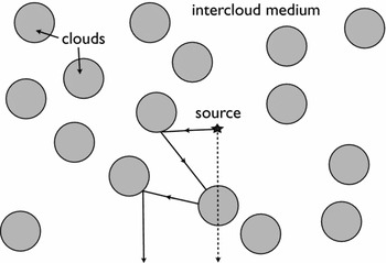
Figure 10. Schematic illustration how a multiphase medium may favour the escape of Lyα line photons over UV-continuum photons: Solid/dashed lines show trajectories of Lyα/UV-continuum photons through clumpy medium. If dust is confined to the cold clumps, then Lyα may more easily escape than the UV-continuum (Credit: from Figure 1 of Neufeld Reference Neufeld1991 ©AAS. Reproduced with permission.).

4.6 Monte carlo radiative transfer

Analytic solutions to the radiative transfer equation (Equation (1)) only exist for a few idealised cases. A modern approach to solve this equation is via Monte-CarloFootnote ¹⁵ , in which scattering of individual photons is simulated until they escape (e.g Loeb & Rybicki Reference Loeb and Rybicki1999; Ahn, Lee, & Lee Reference Ahn, Lee and Lee2001; Zheng & Miralda-Escudé Reference Zheng and Miralda-Escudé2002; Cantalupo et al. Reference Cantalupo, Porciani, Lilly and Miniati2005; Verhamme, Schaerer, & Maselli Reference Verhamme, Schaerer and Maselli2006; Tasitsiomi Reference Tasitsiomi2006; Dijkstra et al. Reference Dijkstra, Haiman and Spaans2006; Semelin, Combes, & Baek Reference Semelin, Combes and Baek2007; Pierleoni, Maselli, & Ciardi Reference Pierleoni, Maselli and Ciardi2009; Kollmeier et al. Reference Kollmeier, Zheng and Davé2010; Faucher-Giguère et al. Reference Faucher-Giguère, Kereš, Dijkstra, Hernquist and Zaldarriaga2010; Barnes et al. Reference Barnes, Haehnelt, Tescari and Viel2011; Zheng et al. Reference Zheng, Cen, Trac and Miralda-Escudé2010; Forero-Romero et al. Reference Forero-Romero, Yepes and Gottlöber2011; Yajima et al. Reference Yajima, Li, Zhu and Abel2012; Orsi et al. Reference Orsi, Lacey and Baugh2012; Behrens & Niemeyer Reference Behrens and Niemeyer2013).Footnote ¹⁶ Details on how the Monte-Carlo approach works can be found in many papers (see e.g. the papers mentioned above, and Chapters 6–8 of Laursen Reference Laursen2010, for an extensive description). To briefly summarise, for each photon in the Monte-Carlo simulations we first randomly draw a position, r _i, at which the photon was emitted from the emissivity profile, a frequency x _i from the Voigt function ϕ(x), and a random propagation direction k _i. We then

1. 1. randomly draw the optical depth τ the photon propagates from the distribution P(τ) = exp ( − τ).

2. 2. convert τ to a physical distance s by inverting the line integral τ = ∫ ^s ₀ dλn _HI(r)σ_α(x[r]), where r = r _i + λk and x = x _i − v(r) · k _i/(v _th). Here, v(r) denotes the 3D velocity vector of the gas at position r.

3. 3. randomly draw velocity components of the atom that is scattering the photon.

4. 4. draw an outgoing direction of the photon after scattering, k _o, from the ‘phase-function’, P(μ) where μ = cos k _i · k _o. The functional form of the phase function depends on whether the photon is resonantly scattered or not (see Section 4.2). It is worth noting that the process of generating the atom’s velocity components and random new directions generates the proper frequency redistribution functions (as well as their angular dependence, see Dijkstra & Kramer Reference Dijkstra and Kramer2012). Unless the photon escapes, we replace the photons propagation direction & frequency and go back to 1).

Observables are then constructed by repeating this process many times and by recording the frequency (when predicting spectra), impact parameter and/or the location of the last scattering event (when predicting surface brightness profileFootnote ¹⁷ ), and possibly the polarisation of each photon that escapes.

5.1 Interstellar radiative transfer

To fully understand Lyα transfer at the interstellar level requires a proper understanding of the multiphase ISM, which lies at the heart of understanding star and galaxy formation. There exist several studies of Lyα transfer through simulated galaxies (Tasitsiomi Reference Tasitsiomi2006; Laursen & Sommer-Larsen Reference Laursen and Sommer-Larsen2007; Laursen et al. Reference Laursen, Sommer-Larsen and Andersen2009a; Barnes et al. Reference Barnes, Haehnelt, Tescari and Viel2011; Verhamme et al. Reference Verhamme, Dubois and Blaizot2012; Yajima et al. Reference Yajima, Li and Zhu2012). It is important to keep in mind that modelling the neutral (outflowing) component of interstellar medium is an extremely challenging task, as it requires simultaneous resolving the interstellar medium and the impact of feedback by star-formation on it (via supernova explosions, radiation pressure, cosmic ray pressure, . . .). This requires (magneto)hydrodynamical simulations with sub-pc resolution (e.g. Cooper et al. Reference Cooper, Bicknell, Sutherland and Bland-Hawthorn2008; Fujita et al. Reference Fujita, Martin, Low, New and Weaver2009). Instead of taking an ‘ab-initio’ approach to understanding Lyα transfer, it is illuminating to use a ‘top-down’ approach in which we try to constrain the broad impact of the ISM on the Lyα radiation field from observations.

Constraints on the escape fraction of Lyα photons, f ^α _esc, have been derived by comparing the intrinsic Lyα luminosity, derived from (dust corrected) UV-derived and/or IR-derived star-formation rates of galaxies, to the observed Lyα luminosity. These analyses have revealed that f ^α _esc is anti-correlated with the dust-contentFootnote ¹⁸ of galaxies (Atek et al. Reference Atek, Kunth and Schaerer2009; Kornei et al. Reference Kornei, Shapley and Erb2010; Hayes et al. Reference Hayes, Schaerer and Östlin2011). This correlation may explain why f ^α _esc increases with redshift from f ^α _esc ~ 1 − 3% at z ~ 0 to about f ^α _esc ~ 30 − 50% at z ~ 6 (e.g. Hayes et al. Reference Hayes, Schaerer and Östlin2011; Blanc et al. Reference Blanc, Adams and Gebhardt2011; Dijkstra & Jeeson-Daniel Reference Dijkstra and Jeeson-Daniel2013, see Figure 11), as the overall average dust content of galaxies decreases towards higher redshifts (e.g. Finkelstein et al. Reference Finkelstein, Papovich and Salmon2012; Bouwens et al. Reference Bouwens, Illingworth and Oesch2012b).

Figure 11. Observational constraints on the redshift-dependence of the volume averaged ‘effective’ escape fraction, f ^eff _esc, which contains constraints on the true escape fraction f ^α _esc (Credit: from Figure 1 of Hayes et al. Reference Hayes, Schaerer and Östlin2011 ©AAS. Reproduced with permission).

It is worth cautioning here that observations are not directly constraining f ^α _esc: Lyα photons that escape from galaxies can scatter frequently in the IGM (or circum-galactic medium) before reaching earth (see Section 5.2). This scattered radiation is typically too faint to be detected with direct observations (Zheng et al. Reference Zheng, Cen, Trac and Miralda-Escudé2010), and is effectively removed from observations. Stacking analyses, which must be performed with great caution (Feldmeier et al. Reference Feldmeier, Hagen and Ciardullo2013), have indeed revealed that there is increasing observational support for the presence of spatially extended Lyα halos around star-forming galaxies (Fynbo, Møller, & Warren Reference Fynbo, Møller and Warren1999; Hayashino et al. Reference Hayashino, Matsuda and Tamura2004; Hayes et al. Reference Hayes, Östlin and Mas-Hesse2005, Reference Hayes, Östlin and Atek2007; Rauch et al. Reference Rauch, Haehnelt and Bunker2008; Östlin et al. Reference Östlin, Hayes and Kunth2009; Steidel et al. Reference Steidel, Erb and Shapley2011; Matsuda et al. Reference Matsuda2012; Hayes et al. Reference Hayes, Östlin and Schaerer2013; Momose et al. Reference Momose, Ouchi and Nakajima2014, but also see Jiang et al. Reference Jiang, Egami and Fan2013). Direct observations of galaxies therefore measure the productFootnote ¹⁹ of f ^α _esc and the fraction of photons that has not been scattered out of the line of sight.

To further understand the impact of RT one would ideally like to compare the properties of scattered Lyα photons (e.g. the spectrum) to that of nebular line photons that did not scatter, such as Hα or [OIII]. For galaxies at z > 2, these observations require spectrographs that operate in the NIR, including e.g. NIRSPEC (McLean et al. Reference McLean, Becklin and Bendiksen1998), LUCIFER (Seifert et al. Reference Seifert, Appenzeller and Baumeister2003), and MOSFIRE (McLean et al. Reference McLean, Steidel and Epps2012).

Simultaneous observations of Lyα & other non-resonant nebular emission lines indicate that Lyα lines typically are redshifted with respect to these other lines by Δv _Lyα. This redshift is more prominent for the drop-out galaxies, in which the average Δv _Lyα ~ 460 km s^{− 1} in LBGs (Steidel et al. Reference Steidel, Erb and Shapley2010; Kulas et al. Reference Kulas, Shapley and Kollmeier2012), which is larger than the shift observed in LAEs, where the average Δv ~ 200 km s^{− 1} (McLinden et al. Reference McLinden, Finkelstein and Rhoads2011; Chonis et al. Reference Chonis, Blanc and Hill2013; Hashimoto et al. Reference Hashimoto, Ouchi and Shimasaku2013; McLinden et al. Reference McLinden, Rhoads and Malhotra2014; Song et al. Reference Song, Finkelstein and Gebhardt2014)Footnote ²⁰ . These observations indicate that outflows affect Lyα radiation while it is escaping from galaxies. This importance of outflows is not surprising: outflows are detected ubiquitously in absorption in other low-ionisation transitions (e.g. Steidel et al. Reference Steidel, Erb and Shapley2010). Moreover, the Lyα photons appear to interact with the outflow, as the Lyα line is redshifted by an amount that is correlated with the outflow velocity inferred from low-ionisation absorption lines (e.g. Steidel et al. Reference Steidel, Erb and Shapley2010; Shibuya et al. Reference Shibuya, Ouchi and Nakajima2014). Scattering of Lyα photons off these outflows provides the photons with a quick route to the wing of the line, where they can escape more easily (see e.g. Shapley et al. Reference Shapley, Steidel, Pettini and Adelberger2003). Indeed, earlier studies had indicated that gas kinematics plays a key role in the escape of Lyα photons from local galaxies (Kunth et al. Reference Kunth, Mas-Hesse, Terlevich, Terlevich, Lequeux and Fall1998; Atek et al. Reference Atek, Kunth, Hayes, Östlin and Mas-Hesse2008). The presence of winds and their impact on Lyα photons is illustrated explicitly in Figure 12.

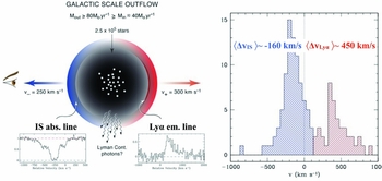
Figure 12. The Figure shows (some) observational evidence for the ubiquitous existence of cold gas in outflows in star-forming galaxies, and that this cold gas affects the Lyα transport: the right panel shows the vast majority of low-ionisation interstellar (IS) absorption lines are blueshifted relative to the systemic velocity of the galaxy, which is indicative of outflows (as illustrated in the left panel, Credit: Figure kindly provided by Max Pettini). Moreover, the right panel (Credit: from Figure 1 of Steidel et al. Reference Steidel, Erb and Shapley2010 ©AAS. Reproduced with permission) illustrates that the Lyα emission line is typically redshifted by an amount that is ~ 2 − 3 times larger than typical blueshift of the IS lines in the same galaxies. These observations are consistent with a scenario in which Lyα photons scatter back to the observer from the far-side of the nebular region (indicated schematically in the left panel).

As modelling the outflowing component in interstellar medium is an extremely challenging task (see above), simple ‘shell-models’ have been invoked to represent the scattering through outflows. In these shell-models, the outflow is represented by a spherical shell with a thickness that is 0.1 × its inner/outer radius. The main properties that characterise the shell are its HI-column density, N _HI, its outflow velocity, v _sh, and its dust content (e.g. Ahn, Lee, & Lee Reference Ahn, Lee and Lee2003; Verhamme et al. Reference Verhamme, Schaerer and Maselli2006, Reference Verhamme, Schaerer, Atek and Tapken2008). For ‘typical’ HI column densities in the range N _HI = 10¹⁹ − 10²¹ cm^{− 2} and v _out ~ a few hundred km s^{− 1}, the red part of the spectrum peaks at ~ 2v _out: photons that scatter ’back’ to the observer on the far side of the Lyα source are Doppler boosted to twice the outflow velocityFootnote ²¹ , where they are sufficiently far in the wing of the absorption cross section to escape from the medium (the cross section at Δv = 200 km s^{− 1} is only σ_α ~ a few times 10^{− 20} cm², see Figure 4). The shell-model can reproduce observed Lyα spectral line shapes remarkably well (e.g. Verhamme et al. Reference Verhamme, Schaerer, Atek and Tapken2008; Schaerer & Verhamme Reference Schaerer and Verhamme2008; Dessauges-Zavadsky et al. Reference Dessauges-Zavadsky, D’Odorico, Schaerer, Modigliani, Tapken and Vernet2010; Vanzella et al. Reference Vanzella, Grazian and Hayes2010).

There are two issues with the shell-models though: (i) gas in the shells has a single outflow velocity and a small superimposed velocity dispersion, while observations of low-ionisation absorption lines indicate that outflows typically cover a much wider range of velocities (e.g. Kulas et al. Reference Kulas, Shapley and Kollmeier2012); and (ii) observations of low-ionisation absorption lines also suggest that outflows -while ubiquitous - do not completely surround UV-continuum emitting regions of galaxies. Observations by Jones et al. (Reference Jones, Ellis, Schenker and Stark2013) show that the maximum low-ionisation covering fraction is 100% in only 2 out of 8 of their z > 2 galaxies (also see Heckman et al. Reference Heckman, Borthakur and Overzier2011, who find evidence for a low covering factor of optically thick, neutral gas in a small fraction of lower redshift Lyman Break Analogues). There is thus some observational evidence that there exist sight lines that contain no detectable low-ionisation (i.e. cold) gas, which may reflect the complex structure associated with outflows which cannot be captured with spherical shells. Two caveats are that (a) the inferred covering factors are measured as a function of velocity (and can depend on spectral resolution, see e.g. Prochaska Reference Prochaska2006, but Jones et al. Reference Jones, Ellis, Schenker and Stark2013 discuss why this is likely not an issue in their analysis). Gas at different velocities can cover different parts of the source, and the outflowing gas may still fully cover the UV emitting source. This velocity-dependent covering is nevertheless not captured by the shell-model; (b) the low-ionisation metal absorption lines only probe enriched cold (outflowing) gas. Especially in younger galaxies it may be possible that there is additional cold (outflowing) gas that is not probed by metal absorption lines.

Recently, Shibuya et al. (Reference Shibuya, Ouchi and Nakajima2014) have shown that Lyα line emission is stronger in galaxies in which the covering factor of low-ionisation material is smaller (see their Figure 10). Similarly, Jones, Stark, & Ellis (Reference Jones, Stark and Ellis2012) found the average absorption line strength in low-ionisation species to decrease with redshift, which again coincides with an overall increase in Lyα flux from these galaxies (Stark et al. Reference Stark, Ellis, Chiu, Ouchi and Bunker2010). Besides dust, the covering factor of HI gas therefore plays an additional important role in the escape of Lyα photons. These cavities may correspond to regions that have been cleared of gas and dust by feedback processes (see Nestor et al. Reference Nestor, Shapley, Steidel and Siana2011, Reference Nestor, Shapley, Kornei, Steidel and Siana2013, who describe a simple ‘blow-out’ model).

In short, dusty outflows appear to have an important impact on the interstellar Lyα radiative process, and give rise to redshifted Lyα lines. Low HI-column density holes further facilitate the escape of Lyα photons from the ISM, and can alter the emerging spectrum such that Lyα photons can emerge closer to the galaxies’ systemic velocities (Behrens, Dijkstra, & Niemeyer Reference Behrens, Dijkstra and Niemeyer2014; Verhamme et al. Reference Verhamme, Orlitova, Schaerer and Hayes2014).

5.2 Intergalactic radiative transfer

As mentioned above, to understand the impact of reionisation on Lyα emitting galaxies, it is important to also understand the impact of the IGM when it has been fully reionised. The transmitted fraction of photons on the blue-side of the Lyα resonance relates to the Gunn-Peterson optical depth (Gunn & Peterson Reference Gunn and Peterson1965),

(22) \begin{equation} \tau _{\rm GP}(\nu _{\rm em})=\int _0^{\infty }ds \hspace{2.84526pt}n_{\rm HI}(s)\sigma _{\alpha }(\nu [s,\nu _{\rm em}]), \end{equation}

where the line integral starts at the galaxy. As photons propagate a proper differential distance ds, the cosmological expansion of the Universe redshifts the photons by an amount dν = −dsH(z)ν/c. Photons that were initially emitted at ν_em > ν_α will thus redshift into the line resonance. Because σ_α(ν) is peaked sharply around ν_α (see Figure 4), we can approximate this integral by taking n _HI(s) and c/ν ≈ λ_α outside of the integral. If we further assume that n _HI(s) corresponds to $\bar{n}_{\rm HI}(z)$ - where $\bar{n}_{\rm HI}(z)=\Omega _{\rm b}h^2(1-Y_{\rm He})(1+z)^3/m_{\rm p}$ denotes the mean number density of hydrogen atoms in the Universe at redshift z - then we obtain

(23) \begin{eqnarray} \tau _{\rm GP}(\nu _{\rm em} > \nu _{\alpha })\eqcellsep=\eqcellsep\frac{\bar{n}_{\rm HI}(z)\lambda _{\alpha }}{H(z)}\int _0^{\infty }d\nu \hspace{2.84526pt}\sigma _{\alpha }(\nu ) \\ \nonumber \eqcellsep=\eqcellsep\frac{\bar{n}_{\rm HI}(z)\lambda _{\alpha }}{H(z)}f_{\alpha }\frac{\pi e^2}{m_{\rm e}c} \approx 7.0 \times 10^5 \Big {(} \frac{1+z}{10}\Big {)}^{3/2}, \end{eqnarray}

where we used that $\int d\nu \hspace{2.84526pt}\sigma (\nu )=f_{\alpha }\frac{\pi e^2}{m_{\rm e}c}$ (e.g. Rybicki & Lightman Reference Rybicki and Lightman1979, p 102). Quasar absorption line spectra indicate that the IGM transmits an average fraction F ~ 85% [F ~ 40%] of Lyα photons at z = 2 [z = 4] which imply ‘effective optical depths of τ_eff ≡ −ln[F] ~ 0.15 [τ_eff ~ 0.9] (e.g. Faucher-Giguère et al. Reference Faucher-Giguère, Prochaska, Lidz, Hernquist and Zaldarriaga2008). The measured values τ_eff ≪ τ_GP which is (of course) because the Universe was highly ionised at these redshifts. A common approach to model the impact of the IGM is to reduce the Lyα flux on the blue side of the Lyα resonance by this observed (average) amount, while transmitting all flux on the red side.

The measured values of F and τ_eff are averaged over a range of frequencies. In detail, density fluctuations in the IGM give rise to enhanced absorption in overdense regions which is observed as the Lyα forest. It is important to stress that galaxies populate overdense regions of the Universe in which: (i) the gas density was likely higher than average, (ii) peculiar motions of gas attracted by the gravitational potential of dark matter halos change the relation between ds and dν, (iii) the local ionising background was likely elevated. We thus clearly expect the impact of the IGMFootnote ²² at frequencies close to the Lyα emission line to differ from the mean transmission in the Lyα forest: Figure 13 shows the transmitted fraction of Lyα photons averaged over a large number of sight lines to galaxies in a cosmological hydrodynamical simulation (Laursen, Sommer-Larsen, & Razoumov Reference Laursen, Sommer-Larsen and Razoumov2011). This Figure shows that infall of over dense gas (and/or retarded Hubble flows) around dark matter halos hosting Lyα emitting galaxies can give rise to an increased opacity of the IGM around the Lyα resonance, and even extending somewhat into the red side of the Lyα line (Santos Reference Santos2004; Dijkstra, Lidz, & Wyithe Reference Dijkstra, Lidz and Wyithe2007; Laursen et al. Reference Laursen, Sommer-Larsen and Razoumov2011). We denote the opacity of the ionised IGM at velocity off-set Δv and redshift z with τ_HII(z, Δv). This provides a source of intergalactic opacity additional to the ‘damping wing’ optical depth, τ_D(z, Δv), that is only relevant during reionisation (see Section 6.2).

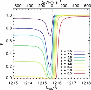
Figure 13. The average fraction of photons that are transmitted though the IGM to the observer as a function of (restframe) wavelength. Each line represents a different redshift. At wavelengths well on the blue side of the line, we recover the mean transmission measured from the Lyα forest. Overdense gas at close proximity to the galaxy increases the IGM opacity close to the Lyα resonance (and causes a dip in the transmission curve, Credit: from Figure 2 of Laursen et al. Reference Laursen, Sommer-Larsen and Razoumov2011 ©AAS. Reproduced with permission).

Because these models predict that the IGM can strongly affect frequencies close to the Lyα resonance, the overall impact of the IGM depends strongly on the Lyα spectral line shape as it emerges from the galaxy. For Gaussian and/or generally symmetric emission lines centred on the galaxies’ systemic velocities, the IGM can transmit as little asFootnote ²³ $\mathcal {T}_{\rm IGM}=10-30\%$ even for a fully ionised IGM (e.g. Dijkstra et al. Reference Dijkstra, Lidz and Wyithe2007; Zheng et al. Reference Zheng, Cen, Trac and Miralda-Escudé2010; Dayal, Maselli, & Ferrara Reference Dayal, Maselli and Ferrara2011; Laursen et al. Reference Laursen, Sommer-Larsen and Razoumov2011). However, when scattering through outflows shifts the line sufficiently away from line centre, the overall impact of the IGM can be reduced tremendously (e.g. Haiman Reference Haiman2002; Santos Reference Santos2004; Dijkstra, Mesinger, & Wyithe Reference Dijkstra, Mesinger and Wyithe2011; Garel et al. Reference Garel, Blaizot and Guiderdoni2012).

We stress that the IGM opacity discussed above originates in mildly over dense (δ = 1 − 20, see Dijkstra et al. Reference Dijkstra, Lidz and Wyithe2007 a), highly ionised gas. Another source of opacity is provided by Lyman-limit systems (LLSs) and Dampled Lyα absorbers (DLAs). The abundance of LLSs increases (weakly) with redshift at z > 3 (e.g. Rahmati et al. Reference Rahmati, Pawlik, Raicevic and Schaye2013), and may strongly affect the IGM opacity at z > 6 (Bolton & Haehnelt Reference Bolton and Haehnelt2013, but see Mesinger et al. Reference Mesinger2014).

6.1 Reionisation

Reionisation refers to the process during which intergalactic gas was transformed from fully neutral to fully ionised. For reviews on the Epoch of Reionisation (EoR) we refer the reader to e.g. Barkana & Loeb (Reference Barkana and Loeb2001), Furlanetto, Oh, & Briggs (Reference Furlanetto, Oh and Briggs2006), and Morales & Wyithe (Reference Morales and Wyithe2010). The EoR is characterised by the existence of a patches of diffuse neutral intergalactic gas, which provides a source of opacity to Lyα photons additional to that discussed in Section 5.2.

Reionisation was likely not a homogeneous process in which the ionisation state of intergalactic hydrogen changed everywhere in the Universe at the same time, and at the same rate. Instead, it was likely an extended highly inhomogeneous process. The first sources of ionizing radiation were highly biased tracers of the underlying mass distribution. As a result, these galaxies were clustered on scales of tens of comoving Mpc (cMpc, Barkana & Loeb Reference Barkana and Loeb2004). The strong clustering of these first galaxies in overdense regions of the Universe caused these regions to be reionised first (e.g. Figure 1 of Wyithe & Loeb Reference Wyithe and Loeb2007), which thus created fluctuations in the ionisation field over similarly large scales. As a result a proper description of the reionisation process requires simulations that are at least 100 cMpc on the side (e.g. Trac & Gnedin Reference Trac and Gnedin2011).

Ideally, one would like to simulate reionisation by performing full radiative transfer calculations of ionising photons on cosmological hydrodynamical simulations. A number of groups have developed codes that can perform these calculations in 3D (e.g. Gnedin Reference Gnedin2000; Sokasian, Abel, & Hernquist Reference Sokasian, Abel and Hernquist2001; Ciardi, Stoehr, & White Reference Ciardi, Stoehr and White2003; Mellema et al. Reference Mellema, Iliev, Alvarez and Shapiro2006; Trac & Cen Reference Trac and Cen2007; Pawlik & Schaye Reference Pawlik and Schaye2008; Finlator, Özel, & Davé Reference Finlator, Özel and Davé2009). These calculations are computationally challenging as one likes to simultaneously capture the large scale distribution of HII bubbles, while resolving the photon sinks (such as Lyman Limit systems) and the lowest mass halos (M ~ 10⁸ M_⊙) which can contribute to the ionising photon budget (see e.g. Trac & Gnedin Reference Trac and Gnedin2011). Modeling reionisation contains many poorly known parameters related to galaxy formation, the ionising emissivity of star-forming galaxies, their spectra etc. Alternative, faster ‘semi-numeric’ algorithms have been developed which allow for a more efficient exploration of the full the parameter space (e.g. Mesinger & Furlanetto Reference Mesinger and Furlanetto2007). These semi-numeric algorithms utilise excursion-set theory to determine if a cell inside a simulation is ionised or not (Furlanetto, Zaldarriaga, & Hernquist Reference Furlanetto, Zaldarriaga and Hernquist2004). Detailed comparisons between full radiation transfer simulations and semi-numeric simulations show both methods produce very similar ionisation fields (Zahn et al. Reference Zahn, Mesinger and McQuinn2011).

The picture of reionisation that has emerged from analytical consideration and large-scale simulations is one in which the early stages of reionisation are characterised by the presence of HII bubbles centred on overdense regions of the Universe, completely separated from each other by a neutral IGM (Furlanetto et al. Reference Furlanetto, Zaldarriaga and Hernquist2004; Iliev et al. Reference Iliev, Mellema and Pen2006; McQuinn et al. Reference McQuinn, Hernquist, Zaldarriaga and Dutta2007). The ionised bubbles grew in time, driven by a steadily growing number of star-forming galaxies residing inside them. The final stages of reionisation are characterised by the presence of large bubbles, whose individual sizes exceeded tens of cMpc (e.g. Zahn et al. Reference Zahn, Mesinger and McQuinn2011). Ultimately these bubbles overlapped (percolated), which completed the reionisation process. The predicted redshift evolution of the ionisation state of the IGM in a realistic reionisation model is shown in Figure 14. This Figure nicely illustrates the inhomogeneous, temporally extended nature of the reionisation process.

Figure 14. The predicted redshift evolution of the ionisation state of the IGM in a realistic reionisation model (Credit: Figure kindly provided by Andrei Mesinger). The white/black represents fully neutral/ionised intergalactic gas. This Figure demonstrates the inhomogeneous nature of the reionisation process which took places over an extended range of redshifts: at z > 16 the first ionised regions formed around the most massive galaxies in the Universe (at that time). During the final stages of reionisation - here at z ~ 9 the IGM contains ionised bubbles several tens of cMpc across.

6.2 Inhomogeneous reionisation & its impact on Lyα

Star-forming galaxies that are luminous enough to be detected with existing telescopes likely populated dark matter halos with masses in excess of M ≳ 10¹⁰ M_⊙. These halos preferentially resides in over dense regions of the Universe, which were reionised earliest. It is therefore likely that (Lyα emitting) galaxies preferentially resided inside these large HII bubbles. Lyα photons emitted by galaxies located inside these HII regions can propagate - and therefore redshift away from line resonance - through the ionised IGM before encountering the neutral IGM. Because of the strong frequency-dependence of the Lyα absorption cross section, these photons are less likely to be scattered out of the line of sight. A non-negligible fraction of Lyα photons may be transmitted directly to the observer, which is illustrated schematically in Figure 15. Inhomogeneous reionisation thus enhances the prospect for detecting Lyα emission from galaxies inside HII bubbles (e.g. Madau & Rees Reference Madau and Rees2000; Haiman Reference Haiman2002; Gnedin & Prada Reference Gnedin and Prada2004; Furlanetto et al. Reference Furlanetto, Zaldarriaga and Hernquist2004; Furlanetto, Zaldarriaga, & Hernquist Reference Furlanetto, Zaldarriaga and Hernquist2006; McQuinn et al. Reference McQuinn, Hernquist, Zaldarriaga and Dutta2007; Mesinger & Furlanetto Reference Mesinger and Furlanetto2008; Iliev et al. Reference Iliev, Shapiro, McDonald, Mellema and Pen2008; Dayal et al. Reference Dayal, Maselli and Ferrara2011; Dijkstra et al. Reference Dijkstra, Mesinger and Wyithe2011; Jensen et al. Reference Jensen, Laursen and Mellema2013; Hutter et al. Reference Hutter, Dayal, Partl and Muller2014). This Figure also illustrates that Lyα photons emitted by galaxies that lie outside of large HII bubbles, scatter repeatedly in the IGM. These photons diffuse outward, and are visible only faint extended Lyα halos (Loeb & Rybicki Reference Loeb and Rybicki1999; Kobayashi, Kamaya, & Yonehara Reference Kobayashi, Kamaya and Yonehara2006; Jeeson-Daniel et al. Reference Jeeson-Daniel, Ciardi and Maio2012).

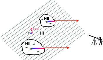
Figure 15. This Figure schematically shows why inhomogeneous reionisation boosts the visibility of Lyα emitting galaxies. During the mid and late stages of reionisation star-forming - and hence Lyα emitting - galaxies typically reside in large HII bubbles. Lyα photons emitted inside these HII bubbles can propagate - and redshift away from line resonance - through the ionised IGM before encountering the neutral IGM. The resulting reduced opacity of the neutral IGM (Equation (30)) to Lyα photons enhances the prospect for detecting Lyα emission from those galaxies inside HII bubbles.

We can quantify the impact of neutral intergalactic gas on the Lyα flux from galaxies following our analysis in Section 5.2. We denote the optical depth in the neutral intergalactic patches with τ_D. We first consider the simplest case in which a Lyα photon encounters one fully neutral patch which spans the line-of-sight coordinate from s_b (‘b’ stands for beginning) to s_e (‘e’ stands for end):

(24) \begin{equation} \tau _{\rm D}(\nu )=\int _{s_b}^{s_e}ds\hspace{2.84526pt}n_{\rm HI}(s)\sigma _{\alpha }(\nu [s]). \end{equation}

Following the analysis of Section 5.2 we change to frequency variables, and recast Equation (24) as

(25) \begin{equation} \tau _{\rm D}(\nu )=\tau _{\rm GP}\frac{\int _{\nu _b(\nu )}^{\nu _e(\nu )}d\nu ^{\prime } \sigma _{\alpha }(\nu ^{\prime })}{\int _0^{\infty }d\nu ^{\prime } \sigma _{\alpha }(\nu ^{\prime })}. \end{equation}

The denominator can be viewed as a normalisation constant, and we can rewrite Equation (25) as

(26) \begin{equation} \tau _{\rm D}(\nu )=\frac{\tau _{\rm GP}}{\sqrt{\pi }} \int _{x_b(\nu )}^{x_e(\nu )} dx\hspace{2.84526pt}\phi (x^{\prime }), \end{equation}

where the factor of $\sqrt{\pi }$ enters because of our adopted normalisation for the Voigt profile ϕ(x).

During the EoR a Lyα photon emitted by a galaxy will generally propagate through regions that are alternating between (partially) neutral and highly ionised. The more general case should therefore contain the sum of the optical depth in separate neutral patches.

(27) \begin{equation} \tau _{\rm D}(\nu )=\frac{1}{\sqrt{\pi }}\sum _i \tau _{\rm GP,i} \hspace{2.84526pt}x_{\rm HI,i}\int _{x_{b,i}(\nu )}^{x_{e,i}(\nu )} dx\hspace{2.84526pt}\phi (x^{\prime }), \end{equation}

where we have placed τ_GP within the sum, because τ_GP depends on redshift as τ_GP∝(1 + z _i)^3/2, and therefore differs slightly for each neutral patch (at redshift z _i).

More specifically, the total optical depth of the neutral IGM to Lyα photons emitted by a galaxy at redshift z _g with some velocity off-set Δv is given by Equation (27) with $x_{b,i} = \frac{-1}{v_{\rm th,i}}[\Delta v+H(z_{\rm g})R_{b,i}/(1+z_{\rm g})]$ , in which R _{b, i} denotes the comoving distance to the beginning of patch ‘i’ (x _{e, i} is defined similarly). Equation (27) must generally be evaluated numerically. However, one can find intuitive approximations: for example, if we assume that (i) x _{HI, i} = 1 for all ‘i’, (ii) z _i ~ z _g, and (iii) that Lyα photons have redshifted away from resonance by the time they encounter this first neutral patchFootnote ²⁴ , then

(28) \begin{equation} \tau _{\rm D}(z_{\rm g},\Delta v)=\frac{\tau _{\rm GP}(z_{\rm g})}{\sqrt{\pi }}\sum _i \hspace{2.84526pt}\Big {(}\frac{a_{\rm v,i}}{\sqrt{\pi }x_{e,i}} - \frac{a_{\rm v,i}}{\sqrt{\pi }x_{b,i}}\Big {)}, \end{equation}

where x _{e, i} = x _{e, i} (Δv) and x _{b, i} = x _{b, i} (Δv). It is useful to explicitly highlight the sign-convention here: photons that emerge redward of the Lyα resonance have Δv > 0, which corresponds to a negative x. Cosmological expansion redshifts photons further, which decreases x further. The $a_{\rm v}/[\sqrt{\pi }x_{b,i}]$ is therefore more negative, and τ_D is thus positive.

One can define the ‘patch-averaged’ neutral fraction $\bar{x}_{\rm D}$ - which is related to the volume filling factor of neutral hydrogen ⟨x _HI⟩ in a non-trivial way (see Mesinger & Furlanetto Reference Mesinger and Furlanetto2008) - as

(29) \begin{eqnarray} \tau _{\rm D}(z_{\rm g},\Delta v)\eqcellsep=\eqcellsep\frac{\tau _{\rm GP}(z_{\rm g})}{\sqrt{\pi }}\bar{x}_{\rm D}\Big {(}\frac{a_{\rm v}}{\sqrt{\pi }x_{e}} - \frac{a_{\rm v}}{\sqrt{\pi }x_{b,1}}\Big {)} \\ \nonumber \eqcellsep\approx\eqcellsep \frac{\tau _{\rm GP}(z_{\rm g})}{\pi }\bar{x}_{\rm D} \frac{a_{\rm v}}{|x_{b,1}|}=\frac{\tau _{\rm GP}(z_{\rm g})}{\pi }\bar{x}_{\rm D}\frac{A_{\alpha }c}{ 4\pi \nu _{\alpha }}\frac{1}{\Delta v_{b,1}}, \end{eqnarray}

where x _e denotes the frequency that photon has redshifted to when it exits from the last neutral patch, while x _{b, 1} denotes the photon’s frequency when it encounters the first neutral patch. Because typically |x _e| ≫ |x _{b, 1}| we can drop the term that includes x _e. We further substituted the definition of the Voigt parameter a _v = A _α/(4πΔν_D), to rewrite x _{b, 1} as a velocity off-set from line resonance when a photon first enters a neutral patch, Δv _{b, 1} = Δv + H(z _g)R _{b, i} /(1 + z _g).

Substituting numbers gives (e.g. Miralda-Escude Reference Miralda-Escude1998; Dijkstra & Wyithe Reference Dijkstra and Wyithe2010)

(30) \begin{equation} \tau _{\rm D}(z_{\rm g},\Delta v)\approx 2.3\bar{x}_{\rm D} \Big {(} \frac{\Delta v_{b,1}}{600\hspace{2.84526pt}{\rm km}\hspace{2.84526pt}{\rm s}^{-1}}\Big {)}^{-1}\Big {(} \frac{1+z_{\rm g}}{10}\Big {)}^{3/2}. \end{equation}

This equation shows that the opacity of the IGM drops dramatically once photons enter the first patch of neutral IGM with a redshift. This redshift may occur partly at the interstellar level, and partly at the intergalactic level: scattering off outflowing materialFootnote ²⁵ at the interstellar level can efficiently redshift Lyα photons by a few hundred km/s (see Section 5.1). Because Lyα photons can undergo a larger cosmological subsequent redshift inside larger HII bubbles, Lyα emitting galaxies inside larger HII bubbles may be more easily detectedFootnote ²⁶ . The presence of large HII bubbles during inhomogeneous reionisation may have drastic implications for the prospects of detecting Lyα emission from the epoch.

7.1 The data

There is increasing observational support for the notion that Lyα emission from star-forming galaxies becomes stronger out to z = 6, after which it suddenly becomes weaker. This applies to both LAEs and drop-out galaxies:

• • Observations of Lyα selected galaxies, also known as Lyα emitters (LAEs), have indicated that the Lyα luminosity functions (LFs) of LAEs do not evolve between z = 3.1 and z = 5.7 (e.g. Hu, Cowie, & McMahon Reference Hu, Cowie and McMahon1998; Ouchi et al. Reference Ouchi, Shimasaku and Akiyama2008). In contrast, the Lyα luminosity of LAEs does evolve at z > 6 (e.g. Kashikawa et al. Reference Kashikawa, Shimasaku and Malkan2006; Ouchi et al. Reference Ouchi, Shimasaku and Furusawa2010; Ota et al. Reference Ota, Iye and Kashikawa2010; Kashikawa et al. Reference Kashikawa, Shimasaku and Matsuda2011), as is shown in the right panel of Figure 16. Importantly, the UV luminosity function of LAEs does not evolve between z = 5.7 and z = 6.5 (see the left panel of Figure 16), which suggests that the reduction of the Lyα luminosity functions at z > 6 is a result of a reduction in Lyα flux coming from these galaxies (as opposed to a reduction simply in their number density, Kashikawa et al. Reference Kashikawa, Shimasaku and Malkan2006, Reference Kashikawa, Shimasaku and Matsuda2011). This evolution appears to continue towards at higher redshifts (z ≳ 7) as well, where Lyα detections are rare (Ota et al. Reference Ota, Iye and Kashikawa2010; Shibuya et al. Reference Shibuya, Kashikawa and Ota2012; Konno et al. Reference Konno, Ouchi and Ono2014, but also see Tilvi et al. Reference Tilvi, Rhoads and Hibon2010), often yielding null-detections (e.g. Clément et al. Reference Clément, Cuby and Courbin2012; Ota et al. Reference Ota, Richard and Iye2012; Jiang et al. Reference Jiang, Bian and Fan2013b; Faisst et al. Reference Faisst, Capak, Carollo, Scarlata and Scoville2014).

  

  Figure 16. Redshift evolution of LAE luminosity functions (LFs) between z = 5.7 and z = 6.5. The left/right panel shows the UV/Lyα LFs. Blue/red solid lines correspond to the acceptable ranges of the luminosity functions. Blue/red dashes lines show best fit Schechter functions assuming a faint end slope α = −1.5. The reduction in the Lyα luminosity function at z > 5.7 (right panel) differs from the observed non-evolution between z = 3.1 − 5.7. Importantly, the reduction in the Lyα LF appears to arise from a reduction in the Lyα flux, as the UV-continuum LF of LAEs does not evolve between z = 5.7 and z = 6.5 (Credit: from Figures 7 and 9 of Kashikawa et al. Reference Kashikawa, Shimasaku and Matsuda2011 ©AAS. Reproduced with permission), we refer the reader to that paper for a full description of all other lines).

• • A similar trend has been observed in drop-out selected galaxies (or Lyman Break Galaxies, or LBGs)Footnote ²⁷ : The fraction of drop-out galaxies with ‘strong’ Lyα emission lines increases within this redshift range (Stark et al. Reference Stark, Ellis, Chiu, Ouchi and Bunker2010), which can quantitatively account for the observed non-evolution of the Lyα LFs within that same redshift range (see e.g. Dijkstra & Wyithe Reference Dijkstra and Wyithe2012). However, at z > 6 the Lyα fraction decreases (Fontana et al. Reference Fontana, Vanzella and Pentericci2010; Stark, Ellis, & Ouchi Reference Stark, Ellis and Ouchi2011; Pentericci et al. Reference Pentericci, Fontana and Vanzella2011; Schenker et al. Reference Schenker, Stark and Ellis2012; Ono et al. Reference Ono, Ouchi and Mobasher2012; Caruana et al. Reference Caruana, Bunker and Wilkins2012, Reference Caruana, Bunker and Wilkins2013; Finkelstein et al. Reference Finkelstein, Papovich and Dickinson2013; Pentericci et al. Reference Pentericci, Vanzella and Fontana2014; Schenker et al. Reference Schenker, Ellis, Konidaris and Stark2014; Tilvi et al. Reference Tilvi, Papovich and Finkelstein2014), in line with observations of the Lyα and UV luminosity functions of LAEs (again quantitatively consistent, see Dijkstra et al. Reference Dijkstra, Wyithe, Haiman, Mesinger and Pentericci2014). This observed evolution is shown in Figure 17.

  

  Figure 17. Redshift evolution of the fraction of drop-out galaxies with ‘strong’ Lyα emission (EW > 25 Å). This fraction, also known as the ‘Lyα’ fraction, increases with redshift out to z = 3, but then decreases (Credit: from Figure 4 of Treu et al. Reference Treu, Schmidt, Trenti, Bradley and Stiavelli2013 ©AAS. Reproduced with permission). This redshift evolution is quantitatively consistent with the redshift evolution of Lyα luminosity functions of LAEs.

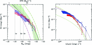
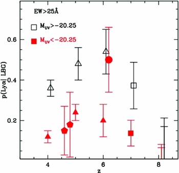
It is therefore safe to conclude that observations of galaxies indicate that the Lyα line has greater difficulty reaching us from galaxies at z > 6 than what expected from observations at z < 6. This is a remarkable result, especially since it has long been predicted to be a key signature of reionisation.

7.2 Interpretation of the data

The sudden reduction in Lyα flux beyond z ~ 6 is naturally associated with the emergence of neutral patches of intergalactic gas. It is thus natural to ask: if this reduction is indeed due to the presence of neutral patches of IGM during the EoR, then how does this reduction compare to what is expected in the context of inhomogeneous reionisation?

The fraction of photons that are transmitted through the IGM during the EoR is given by (e.g. Mesinger et al. Reference Mesinger2014)

(31) \begin{eqnarray} \mathcal {T}_{\rm IGM} \eqcellsep=\eqcellsep \int _{-\infty }^{\infty }d\Delta v\hspace{2.84526pt}J_{\alpha }(\Delta v) \exp [-\tau _{\rm IGM}(z_{\rm g},\Delta v)], \\ \nonumber \tau _{\rm IGM}(z_{\rm g},\Delta v)\eqcellsep=\eqcellsep\tau _{\rm D}(z_{\rm g},\Delta v)+\tau _{\rm HII}(z_{\rm g},\Delta v) \end{eqnarray}

where J _α(Δv) denotes the line profile of Lyα photons as they escape from the galaxy, and τ_D(z _g, Δv) is the given by Equation (28). Equation (31) shows explicitly that there are two components to the IGM opacity: (i) τ_D(z _g, Δv) describes the opacity in diffuse neutral intergalactic patches, and this component is thus unique to the reionisation epoch, and (ii) τ_HII(z _g, Δv) the opacity of the ionised component of the IGM (which can be substantial, see Section 5.2).

To compute τ_D(z _g, Δv) we need to know the spatial distribution of neutral intergalactic patches to compute for a given sightline towards a galaxy. These distributions can be obtained from large-scale radiation transfer simulations, or ‘semi-numerical’ simulations (an example of the large scale ionisation field was shown in Figure 14). We also need to know the location of Lyα emitting galaxies within this simulation. A common assumption is that the Lyα emitting galaxies which are luminous enough to be detectable at these high redshifts with existing telescopes, reside in more massive dark matter halos that existed at the time (M ~ 10¹⁰ − 10¹¹ M _⊙).

Figure 18 shows examples of probability distributions (left panel: differential, right panel: cumulative) for $\mathcal {T}_{\rm IGM}$ for a model for the IGM whose volume averaged neutral fraction is ⟨x _HI⟩ = 91% at z = 8.6 (taken from Dijkstra et al. Reference Dijkstra, Mesinger and Wyithe2011, this redshift was motivated by the claimed detection of a Lyα emission line at this redshift by Lehnert et al. Reference Lehnert, Nesvadba and Cuby2010). The blue dotted line represents a model in which Lyα photons escape from galaxies with a Gaussian emission line [J _α(Δv)] centred on their systemic velocities. The red dashed line & black solid line show models in which the Lyα photons emerge from galaxies with redshifted Lyα line as a result from scattering through an optically thick outflow (see Section 4.4). This redshifted spectral line was modelled by having the photons scatter through a spherical shell model with a column density of N _HI = 10²⁰ cm^{− 2}, and outflow velocity of v _out = 25 km s^{− 1} and v _out = 200 km s^{− 1}. This plot shows that inhomogeneous reionisation allows > 10% of Lyα photons to be transmitted through a highly neutral IGM (which would correspond to an ‘effective’ optical depth ⟨τ_GP⟩ < 2.3) for a non-negligible fraction of galaxies, and that this fraction goes up dramatically when winds affect the Lyα photons on interstellar scales.

Figure 18. These Figures show the probability distributions (left panel: differential, right panel: cumulative) of the fraction of photons that are transmitted through a model for the IGM whose volume averaged neutral fraction is ⟨x _HI⟩ = 91%. The blue dotted line represents a realistic inhomogeneous reionisation model, in which Lyα photons escape from galaxies at their systemic velocities. The red dashed line & black solid line show models in which the Lyα photons emerge from galaxies with a redshift as a result from scattering through an optically thick outflow (see text for details). This plot shows that inhomogeneous reionisation allows > 10% of Lyα photons to be transmitted through a highly neutral IGM (which would correspond to an ‘effective’ optical depth ⟨τ_GP⟩ < 2.3) for a non-negligible fraction of galaxies, and that this fraction goes up dramatically when winds affect the Lyα photons on interstellar scales (Credit: from Figure 2 of Dijkstra et al. Reference Dijkstra, Mesinger and Wyithe2011, ‘The detectability of Lyα emission from galaxies during the epoch of reionisation’, MNRAS, 414, 2139D.).

One can construct similar PDFs for other (volume averaged) neutral fractions (⟨x _HI⟩), and redshifts (z), and estimate how much evolution in ⟨x _HI⟩ is required to explain the observed reduction in the Lyα flux from galaxies at z > 6. For this calculation, we must therefore assume that the observed reduction is entirely due to a changing $\mathcal {T}_{\rm IGM}$ . We stress that radiative transfer in the IGM can (strongly) affect Lyα photons when reionisation is completed (see Section 5.2), but the question we address here is how much additional opacity in the IGM is needed in neutral patches to explain the reduction in Lyα flux at z > 6. For simplicity, we can therefore assumeFootnote ²⁸ that $\mathcal {T}_{\rm IGM}(z=6)=1$ . We further assume that the EW-PDF of the Lyα line in drop-out selected galaxies at z = 6 [P ₆(EW)] is given by an exponential function, i.e. P ₆(EW)∝exp ( − EW/EW_c) (where the scale length EW_c = 50 was chosen to match the data at z = 6). Under these assumptions, we can predict the EW-PDF at z = 7 [P ₇(EW)] to be

(32) \begin{equation} P_7({\rm EW}) \propto \int d\mathcal {T}_{\rm IGM}\hspace{2.84526pt}P_7(\mathcal {T}_{\rm IGM})P_6({\rm EW}/\mathcal {T}_{\rm IGM}). \end{equation}

Example PDFs are shown in Figure 19. Overplotted are data points at z = 7 from Pentericci et al. (Reference Pentericci, Vanzella and Fontana2014). This plot shows that the evolution in the Lyα fraction - when taken at face value - requires a large neutral fraction at z = 7, ⟨x _HI⟩ ~ 0.5 is needed to explain the observed drop at z = 7. What is remarkable about this result, is that the required evolution in ⟨x _HI⟩ is too fast compared to what is expected based on theoretical models of reionisation.

Figure 19. Expected evolution of the (cumulative) EW-PDF for a range of HI volume filling factors, x _HI. The solid line shows the PDF at z = 6, which we assume corresponds to x _HI = 0.0. Increasing x _HI increases the IGM opacity to Lyα photons, which reduces the PDF. Data points are taken from Pentericci et al. (Reference Pentericci, Vanzella and Fontana2014). When taken at face value, the data favours x _HI > 0.5 at z = 7 (Credit: from Figure 4 of Pentericci et al. Reference Pentericci, Vanzella and Fontana2014 ©AAS. Reproduced with permission).

We note that these results were based on ionisation fields generated with semi-numeric models. Similar results have since been obtained by Jensen et al. (Reference Jensen, Laursen and Mellema2013), who used cosmological hydrosimulations in combination with a more complete treatment of radiative transfer of ionizing photons. This agreement is not surprising as semi-numerical methods have been successfully tested against more detailed radiative transfer calculations. It is worth cautioning that the amount of data on z = 7 (and even z < 6) is still small and that, as a consequence, the uncertainties large. Moreover, Taylor & Lidz (Reference Taylor and Lidz2013) have shown that the inhomogeneity of the reionisation process can introduce large variations in the spatial distribution of the Lyα fraction at a fixed x _HI. They further showed that with the current sample sizes of drop-out galaxies, the observations require x _HI > 0.05 (95% CL, although this limit does not include constraints from evolution in the LAE luminosity functions).

7.3 Alternatives & modeling uncertainties

There are alternative physical explanations that can contribute to reducing the Lyα flux from galaxies at z > 6 signature. These can be grouped into two categories:

In the first category, the IGM opacity evolves rapidly beyond z = 6, but not due to the emergence of neutral intergalactic patches. There are several different ways this can happen:

• • The opacity of the ionised intergalactic medium, τ_HII(z, Δv), evolves between z = 5.7 and z = 6.5. The models of Laursen et al. (Reference Laursen, Sommer-Larsen and Razoumov2011) show that the ionised IGM at z = 6.5 can transmit ~ 30% fewer photons than the IGM at z = 5.7. This is related to the fact that the mean density of the Universe at z = 6.5 was ~ 50% higher than at z = 5.7, which translates to an increase in the Gunn-Peterson optical depth by a factor of ~ 1.7 (Dijkstra et al. Reference Dijkstra, Lidz and Wyithe2007). Interestingly, Ouchi et al. (Reference Ouchi, Shimasaku and Furusawa2010) have shown that the evolution in the Lyα luminosity functions of LAEs is consistent with a reduction of ~ 30% in luminosity. It has not been checked whether this model can reproduce the observed drop in the Lyα fraction. It must be noted that these same models predict that the IGM transmits $\mathcal {T}_{\rm IGM}\sim 10-30 \%$ at z ~ 6, which may be at tension with observational constraints on the ‘effective escape fraction’ $f_{\rm esc,eff}\equiv \mathcal {T}_{\rm IGM}f_{\rm esc}$ which prefer f _{esc, eff} ~ 30 − 50% at z = 6 (Hayes et al. Reference Hayes, Schaerer and Östlin2011; Blanc et al. Reference Blanc, Adams and Gebhardt2011; Dijkstra & Jeeson-Daniel Reference Dijkstra and Jeeson-Daniel2013).

• • The opacity in self-shielding Lyman Limit Systems (LLSs) explains the observed evolution. At the end of the EoR, the ionising background may have been substantially smaller than post-reionisation, as a result of the reduced mean free path of ionizing photons. A reduction in the ionizing background reduces the density of gas that can self-shield against it, and therefore increases the number of systems that can self-shield (with N _HI ≳ 10¹⁷ cm^{− 2}), which further reduces the mean free path of ionizing photons. This in turn reduces the ionizing background further etc. The number density of absorption systems with N _HI ≳ 10¹⁷ cm^{− 2} - the LLSs - in our Universe that can self-shield against an ionizing background therefore depends sensitively on the value of the UV (or ionizing) background. Bolton & Haehnelt (Reference Bolton and Haehnelt2013) have shown that LLSs can provide a significant source of opacity to Lyα photons emitted by galaxies, and that the evolution on the number density of LLSs alone can explain the observed drop in the Lyα fraction. The reduced ionising background in these models, still give rise to a significant change in the volume averaged neutral fraction. However, the change required to explain the observed reduction in Lyα flux corresponds only to x _HI ~ 0.1 − 0.2. More recently, Mesinger et al. (Reference Mesinger2014) have shown however that the abundance of LLS may have been overestimated, and they recover the large required change of Δx _HI ~ 0.5.

• • Finally, Finkelstein et al. (Reference Finkelstein, Papovich and Salmon2012) speculate that it may be related to the ratio of the gas accretion rate onto galaxies and their star formation rate, which has been inferred observationally to increase by ~ 40% from z = 6 to z = 7 (Papovich et al. Reference Papovich, Finkelstein, Ferguson, Lotz and Giavalisco2011). Enhanced gas accretion onto galaxies at z = 7 compared to z = 6 at a fixed star formation rate -and hence intrinsic Lyα luminosity - can have two effects: (i) it can increase the opacity of the infalling circum-galactic medium between z = 6 and z = 7 (like the first point discussed above), and (ii) it can cause the line profile emerging from galaxies at z = 7, J _α(ν), to contain a larger fraction of blue-shifted photons as a result of scattering through a more prominent inflowing component. This enhanced fraction of flux on the blue side of the line would make the Lyα flux more subject to scattering in the ionised IGM (see Section 5.2), and hence again enhance its opacity. This possibility has not been investigated quantitatively yet.

In the second category, the intrinsic Lyα luminosity (i.e. prior to scattering through the IGM) decreases at z > 6. Two processes have been considered:

• • The fraction of photons that escape from galaxies decreases at z > 6. Dayal & Ferrara (Reference Dayal and Ferrara2012) argued that dust could mimick a reionisation signature. This requires a non-trivial impact of the dust on Lyα: As mentioned in Section 5.1 f ^α _esc is anti-correlated with the dust content of galaxies. The inferred increase f ^α _esc (or more accurately f ^eff _esc) towards higher redshift can be connected to the reduced dust content of galaxies towards higher redshifts, as inferred from their reddening (e.g. Finkelstein et al. Reference Finkelstein, Papovich and Salmon2012; Bouwens et al. Reference Bouwens, Illingworth and Oesch2012b). The dust content of galaxies keeps decreasing at z > 6. For this reason, Dayal & Ferrara (Reference Dayal and Ferrara2012) invoked an evolution in the dust distribution. In particular, they require a clumpy dust distribution to boost the Lyα escape fraction at z = 6 (see Section 4.5), and not at z = 7. We note that in this model the required boost in the Lyα EW at z = 6 is ~ 1.5. Recent radiative transfer models through clumpy, dusty media have found such boosts to be rare (Laursen et al. Reference Laursen, Duval and Ostlin2013, see Section 4.5).

• • The intrinsic Lyα emission is reduced at z > 6. Lyα emission is powered by recombination following photoionisation inside HII regions, and the Lyα luminosity of a galaxy, L _α∝(1 − f ^ion _esc), where f ^ion _esc denotes the escape fraction of ionizing photons. Direct observational constraints on the escape fraction, and its redshift dependence are still highly uncertain. However, there are several lines of indirect evidence that f ^ion _esc increases with redshift. Measurements of the redshift dependence of the photoionisation rate of the Lyα forest in combination with the observed redshift evolution of the UV-LF of drop-out galaxies, suggest that f ^ion _esc increases quite rapidly with redshift at z ≳ 4 (e.g. Kuhlen & Faucher-Giguère Reference Kuhlen and Faucher-Giguère2012; Mitra, Ferrara, & Choudhury Reference Mitra, Ferrara and Choudhury2013). Dijkstra et al. (Reference Dijkstra, Wyithe, Haiman, Mesinger and Pentericci2014) found that models that incorporate this redshift evolution of f ^ion _esc reduce the required global neutral fraction of Δx _HI ~ 0.2. Moreover, ionizing photons escape efficiently along paths with N _HI ≲ $N_{\rm HI} \lsim 10^{17}$ cm^{− 2}. These same paths enable Lyα photons to escape close to line centre (Behrens et al. Reference Behrens, Dijkstra and Niemeyer2014; Verhamme et al. Reference Verhamme, Orlitova, Schaerer and Hayes2014). If f ^ion _esc indeed increases from z = 6 → 7, then this may cause the average Lyα spectral line shape to shift closer to line-centre. This in turn could increase the opacity of the ionised gas in the IGM (τ_HII(z, Δv), see Section 5.2), and further reduce the required Δx _HI.