


1 INTRODUCTION
The distance of an astronomical object plays an important role in deriving absolute magnitudes of stars and determining the three-dimensional structure of our Galaxy. For nearby stars, Hipparcos (ESA 1997) is the main supplier of the data where a trigonometric parallax has been used. However, for stars at large distances, a photometric parallax is inevitable.
Different methods appeared in the literature related to absolute magnitude determination. Nissen & Schuster (Reference Nissen and Schuster1991) and Laird, Carney, & Latham (Reference Laird, Carney and Latham1988) used the offset from standard main-sequence for the absolute magnitude determination of dwarfs. The studies of Phleps et al. (Reference Phleps, Meisenheimer, Fuchs and Wolf2000) and Chen et al. (Reference Chen2001) are based on the colour–absolute magnitude diagrams of some specific clusters whose metal abundances are adopted as representative of a Galactic population, i.e., thin and thick discs, and halo. Siegel et al. (Reference Siegel, Majewski, Reid and Thompson2002) derived two relations, one for solar-like abundances and another for metal-poor stars, between the MR absolute magnitude and R − I colour index which provide absolute magnitude estimation of dwarfs with different metallicities by means of linear interpolation or extrapolation.
A more recent procedure for absolute magnitude estimation for dwarfs and giants simultaneously is based on the measured atmospheric parameters and the time spent by the star in each region of the H–R diagram. For details of this procedure, we refer to the works of Breddels et al. (Reference Breddels2010) and Zwitter et al. (Reference Zwitter2010).
The most recent absolute magnitude calibrations are those of Karaali, Bilir, & Yaz Gökçe (Reference Karaali, Bilir and Gökçe2012) and Karaali, Bilir & Yaz Gökçe (Reference Karaali, Bilir and Gökçe2013a, Reference Karaali, Bilir and Gökçe2013b). Karaali et al. combined the colour-apparent magnitude diagrams of Galactic clusters with different metal abundances and their distance moduli, and calibrated the MV , Mg , MJ , and M Ks absolute magnitudes of red giants in terms of metallicity. Here, we will apply the same procedure to the dwarfs using the Sloan Digital Sky Survey (SDSS; York et al. Reference York2000) and Two Micron All Sky Survey (2MASS; Skrutskie et al. Reference Skrutskie2006) data, two of the widely used photometric systems in Galactic research. This procedure is different than the ones in Karaali et al. (Reference Karaali, Karataş, Bilir, Ak and Hamzaoğlu2003) and Karaali, Bilir, & Tunçel (Reference Karaali, Bilir and Tunçel2005) where the absolute magnitude was calibrated in terms of the parameter δ0.6, the ultraviolet excess relative to the Hyades cluster, reduced to the intrinsic colour B − V = 0.60 mag. The U ultraviolet magnitude cannot be observed accurately for each star. Whereas, various procedures can be utilized to determine metallicity for a larger set of stars. Hence, for the procedure in this paper, we expect an advantage over the former one.
This paper is the fourth one related to the calibration of absolute magnitudes of stars. The former ones were devoted to red giants, while in this paper the subject is dwarfs. We calibrate the Mg and MJ absolute magnitudes in terms of metallicity. The outline of the paper follows the presentation of the data in Section 2, procedure utilized for calibration in Section 3, and a summary and discussion in Section 4.
2 DATA
We calibrated two different absolute magnitudes, Mg and MJ , in terms of metallicity. Hence, we used two different sets of data. The calibration of g 0 with (g − r)0 is given in Section 2.1, while that for J 0 with (V − J)0 is presented in Section 2.2.
2.1 Data for calibration with SDSS: g 0 × (g − r)0
Our sample consists of M92, M13, M5, NGC 2420, M67, and NGC 6791 stellar clusters with different metal abundance. The SDSS photometric data of the clusters were taken from An et al. (Reference An2008), while the (g − Mg )0 true distance modulus, E(B − V) colour excess, and [Fe/H] iron abundance are from the references in the last column of Table 1. The range of the metallicity is − 2.15 ≤ [Fe/H] ≤ +0.37 dex. The g and g − r fiducials of the stellar clusters adapted from An et al. (Reference An2008) are given in Table 2. As in our previous works, we used RV = 3.1 (Cardelli, Clayton, & Mathis Reference Cardelli, Clayton and Mathis1989) to obtain the total extinction at the V band. Then, we used the equations of Fan (Reference Fan1999) to calculate the total extinction in Ag and the selective absorption in SDSS, E(g − r)/AV = 0.341.
Table 1. Data for the clusters used in the calibration with SDSS.
(1) Gratton et al. (Reference Gratton, Pecci, Carretta, Clementini, Corsi and Lattanzi1997), (2) An et al. (Reference An2008), (3) Brasseur et al. (Reference Brasseur, Stetson, VandenBerg, Casagrande, Bono and Dall’Ora2010)
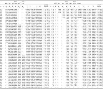
Table 2. g, r magnitudes, g − r, and de-reddened (g − r)0 colours and g 0 magnitudes for the clusters M92, M13, M5, NGC 2420, M67, and NGC 6791 used in the calibration with SDSS.

We fitted the g 0 × (g − r)0 main-sequence of each cluster to a fifth-degree polynomial. The calibration of g 0 is as follows:
 \begin{eqnarray}
g_0=\sum _{i=0}^{5}a_i(g-r)_0^{i}
\end{eqnarray}
\begin{eqnarray}
g_0=\sum _{i=0}^{5}a_i(g-r)_0^{i}
\end{eqnarray}
Table 3. The values of the coefficients ai (i = 0,…,5) in Equation (1).


Figure 1. g 0 × (g − r)0 colour-apparent magnitude diagrams of six stellar clusters used for the absolute magnitude calibration with SDSS.
2.2 Data for calibration with 2MASS: J 0 × (V − J)0
Five clusters with different metallicities, i.e., M92, M13, NGC 6791, 47 Tuc, and NGC 2158, were selected for our programme. The J and V − J data for the first three clusters were taken from Brasseur et al. (Reference Brasseur, Stetson, VandenBerg, Casagrande, Bono and Dall’Ora2010), while those for the clusters of 47 Tuc and NGC 2158 were transformed from the BVRI and gri data, respectively, as explained in the following. For 47 Tuc, we de-reddened the V, B − V, and R − I magnitude and colours of Alcaino et al. (Reference Alcaino, Liller, Alvarado and Wenderoth1990) and transformed them to the (V − J)0 colours by the following equation of Bilir et al. (Reference Bilir, Ak, Karaali, Cabrera-Lavers, Chonis and Gaskell2008):
 \begin{equation}
(V-J)_0=1.557(B-V)_0+0.461(R-I)_0+0.049.
\end{equation}
\begin{equation}
(V-J)_0=1.557(B-V)_0+0.461(R-I)_0+0.049.
\end{equation}
 \begin{equation}
(g-J)_0=1.536(g-r)_0+1.400(r-i)_0+0.488.
\end{equation}
\begin{equation}
(g-J)_0=1.536(g-r)_0+1.400(r-i)_0+0.488.
\end{equation}
 \begin{equation}
V_0=g_0-0.587(g-r)_0 -0.011,
\end{equation}
\begin{equation}
V_0=g_0-0.587(g-r)_0 -0.011,
\end{equation}
 \begin{equation}
(V-J)_0=(g-J)_0-0.587(g-r)_0-0.011.
\end{equation}
\begin{equation}
(V-J)_0=(g-J)_0-0.587(g-r)_0-0.011.
\end{equation}
Table 4. Data for the clusters used in the calibration with 2MASS.
(1) Gratton et al. (Reference Gratton, Pecci, Carretta, Clementini, Corsi and Lattanzi1997), (2) Harris (Reference Harris1996), (3) Alcaino et al. (Reference Alcaino, Liller, Alvarado and Wenderoth1990), (4) Smolinski et al. (Reference Smolinski2011), (5) Arp & Cuffey (Reference Arp and Cuffey1962), (6) Brasseur et al. (Reference Brasseur, Stetson, VandenBerg, Casagrande, Bono and Dall’Ora2010)
Table 5. Colours and magnitudes for the clusters used in the calibration with 2MASS.

We fitted the J 0 × (V − J)0 sequence of four clusters to a fifth-degree polynomial, while a third-degree polynomial was sufficient for NGC 2158 due to less data. The calibration of J 0 is as follows:
 \begin{eqnarray}
J_{0}= \sum _{i=0}^{5}b_{i}(V-J)^{i}_0
\end{eqnarray}
\begin{eqnarray}
J_{0}= \sum _{i=0}^{5}b_{i}(V-J)^{i}_0
\end{eqnarray}
Table 6. Numerical values of the coefficients bi (i = 0, 1, 2, 3, 4, 5).

Figure 2. J 0 × (V − J)0 colour-apparent magnitude diagrams for five clusters used for the MJ absolute magnitude calibration.
3 THE PROCEDURE
3.1 Absolute magnitude as a function of metallicity
We adopted the procedure used in our previous papers (Karaali et al. Reference Karaali, Bilir and Gökçe2013a, Reference Karaali, Bilir and Gökçe2013b) which consists of calibration of an absolute magnitude as a function of metallicity. We calibrated the Mg and MJ absolute magnitudes in terms of metallicity for a given (g − r)0 and (V − J)0 colour, respectively.
3.1.1 Calibration of Mg in terms of metallicity
We estimated the Mg absolute magnitude for the (g − r)0 colours given in Table 7 for the cluster sample in Table 1 by combining the g 0 apparent magnitude evaluated by Equation (1) and the true distance modulus (μ0) of the cluster in question, i.e.,
 \begin{eqnarray}
M_g=g_0-\mu _0.
\end{eqnarray}
\begin{eqnarray}
M_g=g_0-\mu _0.
\end{eqnarray}
Table 7. Mg absolute magnitudes estimated for a set of (g − r)0 colours for six clusters used in the calibration with SDSS.

The Mg × (g − r)0 absolute magnitude–colour diagrams are plotted in Figure 3. The absolute magnitudes of the clusters M13 ([Fe/H] = −1.41 dex) and M5 ([Fe/H] = −1.26 dex) are close to each other for a given colour. Similar case is valid for the clusters NGC 2420 ([Fe/H] = −0.37 dex) and M67 ([Fe/H] = −0.04 dex). However, we used both couples to obtain a better absolute magnitude calibration.

Figure 3. Mg × (g − r)0 colour-magnitude diagram for six clusters used for the absolute magnitude calibration with SDSS.
In this phase, Mg absolute magnitudes can be fitted to the corresponding [Fe/H] metal abundance for a given (g − r)0 colour index and obtain the required calibration. This procedure is executed for the colour indices (g − r)0 = 0.25, 0.40, 0.65, 0.80, 0.95, and 1.20 (Table 8 and Figure 4). The absolute magnitudes in all colour indices are fitted to a second-degree polynomial with (squared) correlation coefficients between R 2 = 0.962 and R 2 = 0.999, where the first one corresponds to the absolute magnitudes for the colour index (g − r)0 = 0.80 mag (but see the following paragraph). A third-degree polynomial (Figure 5) increases the correlation coefficient to R 2 = 1. However, it causes a flat distribution in the metallicity interval − 0.90 ≤ [Fe/H] ≤ −0.40 dex, resulting almost a constant absolute magnitude in this metallicity interval which contradicts the trends of absolute magnitudes for small colour indices, such as (g − r)0 = 0.35 mag, where the correlation coefficient is high, R 2 = 0.991. We shall see in Section 3.2 that the application of the third-degree polynomial in question causes larger residuals than the ones for a quadratic polynomial, ΔM = −0.360 and 0.067 mag, respectively.
Table 8. Mg absolute magnitudes and [Fe/H] metallicities for six (g − r)0 intervals.

Figure 4. Calibration of the absolute magnitude Mg as a function of metallicity [Fe/H] for six colour indices.
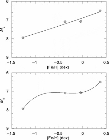
Figure 5. Comparison the trends of the absolute magnitude calibrations with polynomial degrees n = 2 (upper panel) and n = 3 (lower panel) for the colour index (g − r)0 = 0.80 mag.
The number of clusters in the absolute magnitude calibration for the colour indices 0.82 ≤ (g − r)0 ≤ 1.25 mag is only three, i.e., NGC 2420, M67, and NGC 6791 with metallicities [Fe/H] = −0.37, [Fe/H] = −0.04, and [Fe/H] = 0.37 dex, respectively. Additionally, the absolute magnitudes of the clusters NGC 2420 and M67 are close to each other. If we fit a quadratic polynomial to three metallicity and absolute magnitude couples, the segment corresponding to the interval − 0.37 ≤ [Fe/H] ≤ −0.04 dex will perform a concave shape resulting in (estimated) absolute magnitudes larger than the ones for the cluster NGC 2420 which is opposite to the sense of the argument used in our work, i.e., the absolute magnitude of a dwarf with a given metallicity and colour should be brighter than one relatively more metal-poor. Hence, we fitted a linear equation to three metallicity and absolute magnitude couples in question (Figure 6b).

Figure 6. Two fittings to the metallicities and absolute magnitudes for the colour index (g − r)0 = 1.20 dex. (a) a quadratic polynomial to three couples and (b) a linear polynomial to three couples.
The procedure can be applied to any (g − r)0 colour interval for which the sample clusters are defined. The (g − r)0 domains of the clusters are different. Hence, we adopted this interval in our study as 0.25 ≤ (g − r)0 ≤ 1.25 mag where at least three clusters are defined, and we evaluated Mg absolute magnitudes for each colour. Then, we combined them with the corresponding [Fe/H] metallicities and obtained the final calibrations. The general form of the equation for the calibrations is as follows:
 \begin{eqnarray}
M_g = c_0 + c_1 X +c_2 X^2,
\end{eqnarray}
\begin{eqnarray}
M_g = c_0 + c_1 X +c_2 X^2,
\end{eqnarray}
 \begin{eqnarray}
M_g = c_0 + c_1 X,
\end{eqnarray}
\begin{eqnarray}
M_g = c_0 + c_1 X,
\end{eqnarray}
Table 9. Absolute magnitudes estimated for six Galactic clusters and the numerical values of ci (i = 0, 1, 2) coefficients in Equations (8) and (9).
which are valid for the colour interval 0.82 ≤ (g − r)0 ≤ 1.25 are also tabulated in Table 9. The diagrams for the calibrations are not given in the paper because of space constraints. One can use any dataset taken from Table 9 depending on the desire for accuracy, and apply it to stars whose iron abundances are available.
3.1.2 Calibration of MJ in terms of metallicity
We estimated the MJ absolute magnitude for the (V − J)0 colours given in Table 10 for the cluster sample in Table 4 by combining the J 0 apparent magnitude evaluated by Equation (6) and the true distance modulus (μ0) of the cluster in question, i.e.,
 \begin{eqnarray}
M_J= J_0-\mu _0.
\end{eqnarray}
\begin{eqnarray}
M_J= J_0-\mu _0.
\end{eqnarray}
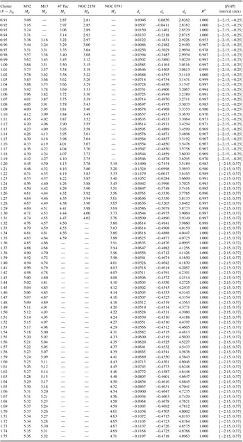
Table 10. MJ absolute magnitudes estimated for a set of (V − J)0 colours for five clusters used for the calibration with 2MASS. The absolute magnitudes with boldface are not considered in the calibration (see text).

The absolute magnitudes versus (V − J)0 colours are plotted in Figure 7. We fitted the MJ absolute magnitudes to the corresponding [Fe/H] metallicity for the following (V − J)0 colour indices and obtained the required calibrations just for the exhibition of the procedure: (V − J)0 = 1.00, 1.15, 1.30, 1.50, and 1.70. The results are given in Table 11 and Figure 8. The absolute magnitudes in all colour indices are fitted to a quadratic polynomial with (squared) correlation coefficients (R 2) between 0.9667 and 1, where the first one corresponds to the absolute magnitudes for the colour index (V − J)0 = 1.15 mag.
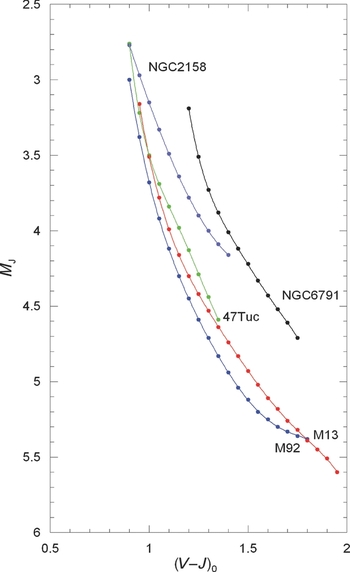
Figure 7. MJ × (V − J)0 colour-absolute magnitude diagrams for five clusters used for the absolute magnitude calibration with 2MASS.

Figure 8. Calibration of the absolute magnitude MJ as a function of metallicity [Fe/H] for five colour indices.
Table 11. MJ absolute magnitudes and [Fe/H] metallicities for five (V − J)0 intervals.
We adopted the interval in 0.90 < (V − J)0 ≤ 1.75 mag, where at least three clusters are defined, for the application of the procedure and we evaluated MJ absolute magnitudes for each colour. Then, we combined them with the corresponding [Fe/H] metallicities and obtained the final calibrations. The general form of the equation for the calibrations is as follows:
 \begin{eqnarray}
M_J = d_0 + d_1 X+ d_2X^2,
\end{eqnarray}
\begin{eqnarray}
M_J = d_0 + d_1 X+ d_2X^2,
\end{eqnarray}
Table 12. MJ absolute magnitudes estimated for five Galactic clusters and the numerical values of di (i = 0, 1, 2) coefficients in Equation (11).
3.2 Application of the procedure
We have two absolute magnitude calibrations, Mg and MJ , in terms of metallicity. Hence, we can apply each of them to a set of data.
3.2.1 Application of the Mg × [Fe/H] calibration
The procedure is applied to four clusters with different metal abundances (M53, M3, M71, and M35). The reason of preferring stellar clusters instead of individual field dwarfs is that clusters provide absolute magnitudes for comparison with the ones estimated by the method. The choice of test clusters as well as the calibrator ones is arbitrary. Hence, we did not involve these clusters into the calibration set but we used them to confirm the robustness of the procedure. In the case of field stars, one needs their distances or trigonometric parallaxes in addition to their g 0 and (g − r)0 data in order to evaluate their absolute magnitudes for their comparison with the ones estimated by the procedure in our work. However, such stars are rare in the literature. The parameters of stellar clusters and (g, g − r) photometric data are given in Tables 13 and 14, respectively. The colour-apparent magnitude diagrams of the Galactic clusters used for the application of the procedure are shown in Figure 9. The g and the g − r data of the clusters M53, M3, and M71 are taken from An et al. (Reference An2008), whereas those of M35 are transformed from the V and B − V data in von Hippel et al. (Reference Hippel, Steinhauer, Sarajedini and Deliyannis2002) by the reduced transformation equations of Chonis & Gaskell (Reference Chonis and Gaskell2008) given in the following:
 \begin{eqnarray}
g=V+0.642\times (B-V)-0.135,\nonumber \\
g-r= 1.094\times (B-V)-0.248.
\end{eqnarray}
\begin{eqnarray}
g=V+0.642\times (B-V)-0.135,\nonumber \\
g-r= 1.094\times (B-V)-0.248.
\end{eqnarray}
Table 13. Data for the clusters used for the application of the procedure with SDSS.
(1) Smolinski et al. (Reference Smolinski2011), (2) Ferro et al. (Reference Ferro2011), (3) An et al. (Reference An2008), (4) Saad & Lee (Reference Saad and Lee2001), (5) Di Criscienzo, Marconi, & Caputo (Reference Criscienzo, Marconi and Caputo2004), (6) Sarajedini, Mathieu, & Platais (Reference Sarajedini, Mathieu and Platais2003)
Table 14. Fiducial dwarf sequence for the galactic clusters used in the application of the procedure with SDSS.

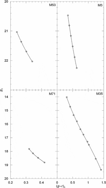
Figure 9. g 0 × (g − r)0 colour-apparent magnitude diagrams for the Galactic clusters used for the application of the procedure.
The reason of this choice is to obtain the g and g − r data for a relatively metal rich cluster with a large colour range. The metallicity of M35 is [Fe/H] = −0.16 dex, and it covers the colour range of − 0.30 ≤ (g − r)0 ≤ 1.40 mag. However, the application could be carried out for the colour interval 0.35 ≤ (g − r)0 ≤ 1.25 mag, due to the restriction of our calibrations for the metallicity [Fe/H] = −0.16 dex (see Table 9).
We evaluated the Mg absolute magnitude by Equation (8) for a set of (g − r)0 colour indices where the clusters are defined. The results are given in Table 15. The columns refer to (1) (g − r)0, colour index; (2) (Mg ) ev , the absolute magnitude estimated by the procedure; (3) (Mg ) cl , absolute magnitude for a cluster estimated by its colour-magnitude diagram; and (4) ΔM, absolute magnitude residuals. Also, the metallicity for each cluster is indicated near the name of the cluster. The differences between the absolute magnitudes estimated by the procedure presented in this study and those evaluated via colour–magnitude diagrams of the clusters (the residuals) lie between − 0.15 and + 0.12 mag. The mean and the standard deviation of the residuals are < ΔMg > = − 0.002 and σ = 0.065 mag, respectively. The distribution of the residuals is given in Table 16 and Figure 10.
Table 15. Absolute magnitudes ((Mg ) ev ) and residuals (ΔM) estimated by the procedure explained in our work. (Mg ) cl denotes the absolute magnitude evaluated by means of colour - magnitude diagram of the cluster.
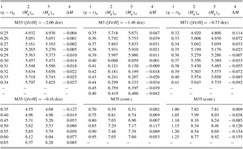
Table 16. Distribution of the residuals. N denotes the number of stars.

Figure 10. Histogram of the residuals.
The linear (Equation (9)) is valid for the colours (g − r)0 ≥ 0.82. Hence, we could apply it to only cluster M35. We used the c 1 and c 0 coefficients in Table 9 and evaluated the (Mg ) ev absolute magnitudes for nine (g − r)0 colours, i.e. 0.85, 0.90, 0.95, 1.0, 1.05, 1.10, 1.15, 1.20, and 1.25 mag. Then, we compared them with the corresponding ones, (Mg ) cl . The mean of the residuals and the standard deviation for this set of data are < ΔM > = − 0.102 and σ = 0.094 mag, respectively.
3.2.2 Application of the MJ × [Fe/H] calibration
We applied the procedure to the cluster M5 and to a set of field stars with solar metallicity as explained in the following. The reason of choosing a cluster is that it provides absolute magnitudes for comparison with the ones estimated by the procedure. The colour excess, E(B − V) = 0.03 mag and the metallicity [Fe/H] = −1.40 dex of the cluster are taken from Reid (Reference Reid1997), while for the apparent distance modulus we adopted the one of Brasseur et al. (Reference Brasseur, Stetson, VandenBerg, Casagrande, Bono and Dall’Ora2010), μ = 14.45 mag. Sarajedini et al. (Reference Sarajedini, Brandt, Grocholski and Tiede2004) published the 2MASS magnitudes, V magnitudes, metallicities, and parallaxes of 54 field stars. Parallaxes provide absolute magnitudes for comparison with the ones estimated by our procedure, and this is the reason of choosing this sample of stars. The range of the metallicity is − 0.45 ≤ [Fe/H] ≤ +0.35 dex, i.e., the stars are of solar metallicity. Hence, their combination with (relatively) metal-poor stars in cluster M5 provides a good sample for the application of the procedure. Two stars, Hip 69301 and Hip 84164, are omitted due to their large relative parallax errors, σπ/π = 0.16 and 0.09, respectively. Also, six stars which fall off the colour domain of our procedure, i.e. (V − J)0 > 1.75 mag, could not be included into our programme. The V − J colours and J magnitudes of M5 cluster were de-reddened by the equations given in Section 3.1.2, while all the magnitudes in Sarajedini et al. (Reference Sarajedini, Brandt, Grocholski and Tiede2004) were assumed as unaffected from the interstellar extinction due to the proximity of the field stars to the Sun, d < 75 pc. The results are given in Table 17 and Figure 11. The data of the field stars in columns (1)–(6) are original, while those in (7)–(9) are evaluated in this paper. The distance (d) was evaluated by using the corresponding parallax, and the absolute magnitude MJ was calculated by the well known Pogson formula.
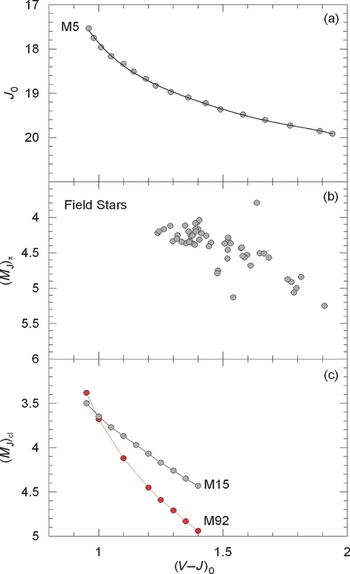
Figure 11. J 0 × (V − J)0 colour-apparent magnitude diagram of the cluster M5 (panel a), distribution of the field stars with solar metallicity in the (V − J)0 colour versus (MJ )π absolute magnitude diagram (panel b), and deviation of the (V − J)0 colour (MJ ) cl absolute magnitude diagram of the cluster M15 (brighter magnitudes) from the one of M92 (fainter magnitudes).
Table 17. Data for the cluster M5 and the field stars used for the application of the procedure with 2MASS.

We evaluated the MJ absolute magnitude by Equation (11) for two sets of (V − J)0 colour indices. The first set covers the domain of the cluster M5 (Table 18a), while the second one consists of (V − J)0 colour indices of the field stars (Table 18b). The columns in Table 18a refer to (1) (V − J)0 colour index, (2) (MJ ) cl , the absolute magnitude estimated by the combination of the colour–magnitude diagram and the true distance modulus of the cluster M5, (3) (MJ ) ev , the absolute magnitude estimated by the procedure, and (4) ΔM, absolute magnitude residuals. For metallicity, we adopted the one of cluster M5, i.e. [Fe/H] = −1.40 dex. The columns in Table 18b refer to (1) (V − J)0 colour index of the field star, (2) (MJ )π, the absolute magnitude estimated by the parallax of the field star, (3) [Fe/H], the metallicity of the field star, (4) (MJ ) ev , the absolute magnitude estimated by the procedure, and (5) ΔM, absolute magnitude residuals. The total residuals lie between − 0.29 and + 0.39 mag. The extreme residuals ΔM = −1.03 and +0.56 mag which are marked in boldface in Table 18b correspond to stars Hip 84164 and Hip 69301 whose relative parallax errors are high, as mentioned above. Hence, they are not considered in the calculations of the mean residual and standard deviation. However, the range of 87% of them is rather shorter, i.e. − 0.20 < ΔM ≤ +0.20 mag. The mean and the standard deviation of all residuals, except the two extreme ones, are < ΔMJ > =0.05 and σ = 0.13 mag. The distribution of the residuals is also given in Table 19 and Figure 12. We state that the cluster fiducials provide more accurate absolute magnitudes than the ones for the field stars. Actually, the mean and the standard deviation of the residuals for the fiducials are < ΔMJ > =0.04 and σ = 0.05 mag, whereas those for the field stars are < ΔMJ > =0.06, σ = 0.16 mag, respectively.
Table 18. Absolute magnitudes (MJ ) ev and residuals ΔM estimated by the procedure explained in our work. (MJ ) cl and (MJ )π denote the absolute magnitudes evaluated by means of the colour-magnitude diagram of the M5 cluster and the parallax of the field star, respectively.

Table 19. Distribution of the residuals. N denotes the number of stars.
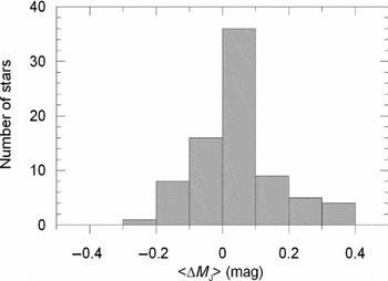
Figure 12. Histogram of the residuals.
4 SUMMARY AND DISCUSSION
We presented two absolute magnitude calibrations for dwarfs based on the colour magnitude diagrams of Galactic clusters with different metallicities. For the calibration of Mg , we used the clusters M92, M13, M5, NGC 2420, M67, and NGC 6791. We combined the calibrations between g 0 and (g − r)0 for each cluster with their true distance modulus and evaluated a set of absolute magnitudes for the (g − r)0 range of each cluster. Then, we fitted the Mg absolute magnitudes in terms of the iron metallicity, [Fe/H], by a quadratic polynomial for a given (g − r)0 colour index. Our absolute magnitude calibrations cover the range 0.25 ≤ (g − r)0 ≤ 1.25 mag.
We applied the procedure to another set of Galactic cluster, i.e. M53, M3, M71, and M35 and compared the absolute magnitudes estimated by this procedure with those evaluated via a combination of the fiducial g 0, (g − r)0 sequence and the true distance modulus for each cluster. The residuals lie between − 0.15 and + 0.12 mag, and their mean and standard deviations are < ΔM > = − 0.002 and σ = 0.065 mag. The range of the residuals estimated for the red giants with SDSS was − 0.28 ≤ ΔM ≤ +0.43 mag (Karaali et al. Reference Karaali, Bilir and Gökçe2013a), larger than the one for the dwarfs estimated in this study. Also, their mean and standard deviation were larger, i.e. < ΔM > =0.169 and σ = 0.140. The difference between two sets of residuals originates mainly from the different trends of the colour–magnitude diagrams of red giants and dwarfs, i.e., the colour–magnitude diagram of red giants for a given cluster is steeper than the one for dwarfs of the same cluster, and any error in (g − r)0 results in larger colour errors within the steeper diagram.
The range of the (B − V)0 colour in Karaali et al. (Reference Karaali, Karataş, Bilir, Ak and Hamzaoğlu2003) who estimated absolute magnitudes for dwarfs by absolute magnitude offsets is 0.3 ≤ (B − V)0 ≤ 1.1 mag which corresponds to 0.1 ≤ (g − r)0 ≤ 0.9 mag, shorter than the one cited in our study, i.e. 0.25 ≤ (g − r)0 ≤ 1.25 mag. That is, there is an improvement on our procedure with respect to the one of Karaali et al. (Reference Karaali, Karataş, Bilir, Ak and Hamzaoğlu2003).
For the calibration of MJ , we used the clusters M92, M13, 47 Tuc, NGC 2158 and NGC 6791. We combined the calibrations between J 0 and (V − J)0 for each cluster with their true distance modulus and evaluated a set of absolute magnitudes for the (V − J)0 range of each cluster. Then, we calibrated the MJ absolute magnitudes in terms of the iron metallicity, [Fe/H], by a quadratic polynomial for all cluster. Our absolute magnitude calibrations cover the range 0.90 < (V − J)0 ≤ 1.75 mag.
This is our fourth paper devoted to the calibration of the absolute magnitudes based on the colour–magnitude diagrams of Galactic clusters, and it is the first time that we used a set of field stars, additional to the Galactic cluster M5 ([Fe/H] = −1.40 dex), for the application of the MJ × [Fe/H] calibration. We tried to apply the procedure to a metal-poor cluster, i.e., M15 whose metallicity is close to the one of M92. But we noticed that the residuals were decreasing systematically from ΔM = 0.51 to ΔM = −0.26 mag in the colour range 0.95 ≤ (V − J)0 ≤ 1.40 mag. Comparison of the absolute magnitude–colour diagrams of the clusters M92 and M15 (Figure 11c) revealed that the reason for the systematic variation of the residuals is due to the fiducial sequence of the cluster M15. Actually, although the absolute magnitudes evaluated for M92 and M15 for the colour (V − J)0 = 0.95 mag are close to each other, the absolute magnitudes of M15 deviate from the ones of M92 up to ΔM = 0.51 mag at redder colours. Hence, the systematic residuals in question do not originate from our procedure but they are due to the fiducial sequence of the cluster M15. The fiducial sequences of the clusters M92 and M15 are taken from the same source, i.e. Brasseur et al. (Reference Brasseur, Stetson, VandenBerg, Casagrande, Bono and Dall’Ora2010). The metallicities for both clusters are given as [Fe/H] = −2.4 dex in the same paper. Additionally, they have the same age, a bit less than 13 Gyr (Salaris, degl’Innocenti, & Weiss Reference Salaris, degl’Innocenti and Weiss1997). Hence, the problem related to the discrepancy between the two fiducial sequences could not be solved.
We compared the absolute magnitudes estimated by the procedure explained in our paper with those evaluated either by combination of the J 0, (V − J)0 fiducial sequence of the cluster M5 and its true distance modulus or by the J 0 apparent magnitude and the distance of the field star in question. The total residuals lie between − 0.29 and + 0.39 mag. However, the range of 87% of them is rather shorter, i.e. − 0.20 < ΔM ≤ +0.20 mag. The mean and the standard deviation of all residuals are < ΔM > =0.05 and σ = 0.13 mag. However, we state that the cluster fiducials provide more accurate absolute magnitudes than the ones for the field stars. Thus, the absolute magnitude MJ of a dwarf would be determined with an accuracy of ΔM < 0.2 mag. The mean and standard deviation of the residuals estimated with the same photometry (V, J) for red giants were < ΔM > =0.137 and σ = 0.080 mag (Karaali et al. Reference Karaali, Bilir and Gökçe2013b) which indicates that the absolute magnitudes of dwarfs would be determined with better accuracy. The reason of this improvement is the same as stated for the absolute magnitude Mg . The calibration of Mg and MJ in terms of [Fe/H] is carried out in steps of 0.01 mag. A small step is necessary to isolate an observational error on g − r and V − J plus an error due to reddening. The origin of the mentioned errors shows the trend of the dwarf sequence. However, we note that the dwarf sequence is not steep. Hence, contrary to the red giant branch sequence Karaali et al. (Reference Karaali, Bilir and Gökçe2013a), an error in (g − r) or (V − J) does not imply a large change in the absolute magnitude.
The ci and di (i = 0, 1, 2) coefficients in Tables 9 and 12, respectively, are colour-dependent. Additionally, it seems that there is a smooth relation between a given ci or di coefficient and the (g − r) and (V − J) colour. We confirmed this argument by plotting each ci coefficient versus (g − r)0 colour. Actually, each panel in Figure 13 consists of a set of smooth relations with breaks at (g − r)0 colours where the number of clusters employed in the [Fe/H] calibrations changes. It is interesting, the mentioned breaks in the panel c 0 versus (g − r)0 are so small that one can assume a continuous relation for the whole colour interval, i.e. 0.25 ≤ (g − r)0 ≤ 1.25 mag. The mentioned relation originates from the fact that Mg = c 0 for [Fe/H] = 0 dex.
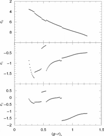
Figure 13. Variation of c 0, c 1, and c 2 coefficients with colour index (g − r)0 in three panels.
The procedure for absolute magnitude calibration for dwarfs in Karaali et al. (Reference Karaali, Karataş, Bilir, Ak and Hamzaoğlu2003) is based on the absolute magnitude offset which is defined as a function of ultraviolet excess. However, ultraviolet excess can not be provided easily with SDSS, especially for late-type stars, and this parameter has not been defined in 2MASS system. Whereas, the procedure in this study is metallicity-dependent, and metallicity values come from detailed analysis of individual stars using high-resolution spectroscopy in large surveys which are in operation, such as RAVE, SEGUE, GAIA-ESO, and APOGEE or which will be started in the near future, such as GALAH.
SDSS and 2MASS are two of the widely used photometric systems in the Galactic researches. Also, our procedure covers dwarfs with a large metallicity and age range. The metallicity range is − 2.15 ≤ [Fe/H] ≤ 0.37 dex in both systems, while the age ranges are defined by the clusters used for the calibrations in SDSS and 2MASS, i.e. 4 ≤ t ≤ 13.2 and 2 ≤ t ≤ 13.2 Gyr, respectively, where 2, 4 and 13.2 Gyr are the ages of the clusters NGC 2158, M67 and M92. The age of the cluster NGC 2158 is taken from Carraro, Girardi, & Marigo (Reference Carraro, Girardi and Marigo2002), while those for the clusters M67 and M92 were estimated in Karaali et al. (Reference Karaali, Bilir and Gökçe2012). Additionally, the mean residuals and standard deviations in the application of two absolute magnitude calibrations, Mg and MJ , are small. Hence, the procedure presented in this paper can be applied with a good accuracy to large samples of dwarf stars in Galactic-structure Projects.
We stated in our previous papers (Karaali et al. Reference Karaali, Bilir and Gökçe2012) that our absolute magnitude calibrations are age-restricted, i.e., they cover the stars with ages in the range defined by the youngest and oldest clusters used in the calibration. We applied the calibration Mg × [Fe/H] to two clusters, NGC 3680 and NGC 2158, younger than 4 Gyr to test the age range in the SDSS system. We used the V and B − V data of the cluster NGC 3680 in Kozhurina-Platais et al. (Reference Kozhurina-Platais, Demarque, Platais, Orosz and Barnes1997) and reduced them to the g 0 magnitude and (g − r)0 colour by means of the equations of Chonis & Gaskell (Reference Chonis and Gaskell2008) given in Section 3.2.1, after necessary corrections for interstellar extinction. The colours and magnitudes of the cluster NGC 2158 taken from Smolinski et al. (Reference Smolinski2011) are already in the SDSS system. The Mg × [Fe/H] calibration could be applied to nine stars in NGC 3680 and 10 fiducials in NGC 2158, and the absolute magnitude residuals for each set of data were estimated. The mean residuals are very similar and rather high, i.e. < ΔM > =1.25 mag for 9 stars and < ΔM > =1.20 mag. for 10 fiducials, which shows that the calibration in question is limited with the age of the youngest cluster used for the calibration, i.e., 4 Gyr. The metallicities of the clusters NGC 3680 and NGC 2158 are close to the one of M67 whose age is 4 Gyr, while the ages of the first two clusters are different than the one of M67. A similar test can be carried out for the MJ × [Fe/H] calibration. Hence, we can argue that our absolute magnitude calibrations are better defined in terms of ranges in age. The colour excesses, distance moduli, metallicities, and ages of the clusters are presented in Table 20. However, the magnitudes and colours used in the evaluation of absolute magnitude residuals are not given in the paper because of space constraints.
Table 20. Data for two young clusters.
(1) Cummings et al. (Reference Cummings, Deliyannis, Anthony-Twarog, Twarog and Maderak2012), (2) Eggen (Reference Eggen1969), (3) Smolinski et al. (Reference Smolinski2011), (4) Saad & Lee (Reference Saad and Lee2001).
ACKNOWLEDGMENTS
The authors would like to thank the anonymous referee who provided valuable comments and for improving the manuscript. This research has made use of NASA(National Aeronautics and Space Administration)’s Astrophysics Data System and the SIMBAD Astronomical Database, operated at CDS, Strasbourg, France.


