1 INTRODUCTION
All sky surveys have a great impact on our understanding of the Galactic structure. The optical and longer wavelength surveys give detailed information about the Galactic halo, and Galactic disc and bulge, respectively. The Sloan Digital Sky Survey (SDSS; York et al. Reference York2000) is one of the most widely used sky surveys. Also, it is the largest photometric and spectroscopic survey in the optical wavelengths. Another widely used sky survey is the Two Micron All Sky Survey (2MASS; Skrutskie et al. Reference Skrutskie2006), which imaged the sky across near-infrared wavelengths. The third sky survey, which is an astrometrically and photometrically important survey, is Hipparcos (Perryman et al. Reference Perryman1997), re-reduced by van Leeuwen (Reference van Leeuwen2007).
SDSS is based on two sets of passbands, i.e. u′g′r′i′z′ and ugriz. For the first set, the standard Sloan photometric system was defined on the 1m telescope of the USNO Flagstaff Station (Smith et al. Reference Smith2002), while a 2.5 m telescope was used for the second passband set (Fukugita et al. Reference Fukugita, Ichikawa, Gunn, Doi, Shimasaku and Schneider1996; Gunn et al. Reference Gunn1998; Hogg et al. Reference Hogg, Finkbeiner, Schlegel and Gunn2001). The two sets of passbands are very similar, but not quite identical. However, one can use the transformation equations in the literature to make necessary transformations between two systems (cf. Rider et al. Reference Rider, Tucker, Smith, Stoughton, Allam and Neilsen2004).
It has been customary to derive transformation equations between a newly defined photometric system and the traditional ones, such as the Johnson-Cousins UBVRcIc system. Several transformations can be found in the literature related SDSS photometric system (Smith et al. Reference Smith2002; Karaali, Bilir, & Tunçel Reference Karaali, Bilir and Tunçel2005; Bilir, Karaali, & Tunçel Reference Bilir, Karaali and Tunçel2005; Rodgers et al. Reference Rodgers, Canterna, Smith, Pierce and Tucker2006; Jordi, Grebel, & Ammon Reference Jordi, Grebel and Ammon2006; Chonis & Gaskell Reference Chonis and Gaskell2008; Bilir et al. Reference Bilir, Ak, Karaali, Cabrera-Lavers, Chonis and Gaskell2008). All these transformations are devoted to dwarfs, the most populated luminosity class in our Galaxy. The two transformations which are carried out for red giants are those of Yaz et al. (Reference Yaz, Bilir, Karaali, Ak, Coşkunoğlu and Cabrera-Lavers2010) and Karaali & Yaz Gökçe (Reference Karaali and Gökçe2013).
Yaz et al. (Reference Yaz, Bilir, Karaali, Ak, Coşkunoğlu and Cabrera-Lavers2010) used the JHKs , BVI, and gri magnitudes in the 2MASS (Cutri et al. Reference Cutri2003), reduced Hipparcos’ (van Leeuwen Reference van Leeuwen2007) and Ofek's (Reference Ofek2008) catalogues and identified two samples of red giants by matching them with the Cayrel de Strobel, Soubiran, & Ralite's (Reference de Strobel, Soubiran and Ralite2001) spectroscopic catalogue which contains the surface gravity logg, a parameter available for dwarf-giant separation. The first sample of stars (91 giants) was used for the transformations between JHKs and BVI, while the second one (82 giants) was devoted to transformations between JHKs and gri. The transformations of Karaali & Yaz Gökçe (Reference Karaali and Gökçe2013) are based on synthetic UBV colours of Buser & Kurucz (Reference Buser and Kurucz1992) and synthetic ugr colours of Lenz et al. (Reference Lenz, Newberg, Rosner, Richards and Stoughton1998). They are metallicity and two colours dependent. Three sets of transformation equations are obtained, i.e. for [M/H] = 0, −1, −2 dex, which can be interpolated/extrapolated to different metallicities. The advantage of these transformations is that they can be used to extend the colour ranges of the observed u − g and g − r colours which are restricted due to the saturation of the SDSS magnitudes.
In this study, we present transformation equations between either of the most widely used sky surveys, SDSS g′r′i′, and BVRc for giants. The equations are based on the data which were observed and reduced by a team who are included as co-authors in this paper. The sections are organised as follows. Data are presented in Section 2. Section 3 is devoted to the transformation equations and their application and a summary and discussions are given in Section 4.
2 THE DATA
2.1 Observations
The sample consists of fairly bright 80 giants identified and collected by their surface gravities and effective temperatures in the Pastel catalogue (Soubiran et al. Reference Soubiran, Le Campion, de Strobel and Caillo2010): (i) 2 ⩽ logg (cm s− 2) ⩽ 3, (ii) 4000 < Teff (K) < 16000. The sample stars cover a large range of metallicities, i.e. − 4 ⩽ [Fe/H] ⩽ 0.5 dex. The sample stars were observed at least three exposures in each filter used. The observations were carried out at 1m RC telescope (T100) at TÜBİTAK National Observatory (TUG)Footnote 1 at Bakırlıtepe, Antalya, in Turkey from 2011 July through 2012 September. Table 1 summarises the journal of observations. The columns indicate the dates, the number of nights, and the number of observing sets at g′r′i′ and BVRc filters both for the sample and standard stars.
Table 1. Observing runs at the TUG T100 telescope. Number of frames for giants and standard stars are given in the last four columns according to the filter sets used.

Standard reduction techniques were performed with Image Reduction and Analysis Facility (IRAF)Footnote 2 . Sky observations during the twilight were used in the flat field corrections. As the dark current level of the CCD camera is very low (0.0002 e− pixel− 1 s− 1) and the exposure times during observing runs are not long, dark current corrections were not applied. Instrumental magnitudes were obtained through aperture photometry using standard IRAF software packages. The instrumental magnitudes and colours were transformed to the standard photometric systems following the procedures described below. The following equations were used for the transformation of the instrumental magnitudes and colours of giant stars to the standard magnitudes and colours:
 \begin{eqnarray}
V &=& v-k_V\times X_v +\epsilon _V \times (B-V)+\zeta _V, \\
\end{eqnarray}
\begin{eqnarray}
V &=& v-k_V\times X_v +\epsilon _V \times (B-V)+\zeta _V, \\
\end{eqnarray}
 \begin{eqnarray}
B-V&=&\mu \times [(b-v)-(k_{BV} \times X_{BV})]+\zeta _{BV}, \\
\end{eqnarray}
\begin{eqnarray}
B-V&=&\mu \times [(b-v)-(k_{BV} \times X_{BV})]+\zeta _{BV}, \\
\end{eqnarray}
 \begin{eqnarray}
V-R_c&=&\rho \times [(v-r_c)-(k_{VR_c} \times X_{VR_c})]+\zeta _{VR_c}, \\
\end{eqnarray}
\begin{eqnarray}
V-R_c&=&\rho \times [(v-r_c)-(k_{VR_c} \times X_{VR_c})]+\zeta _{VR_c}, \\
\end{eqnarray}
 \begin{eqnarray}
g^{\prime }&=&g-k_g \times X_g+\epsilon _g \times (g-r)+\zeta _{g}, \\
\end{eqnarray}
\begin{eqnarray}
g^{\prime }&=&g-k_g \times X_g+\epsilon _g \times (g-r)+\zeta _{g}, \\
\end{eqnarray}
 \begin{eqnarray}
g^{\prime }-r^{\prime }&=&\kappa \times [(g-r)-(k_{gr} \times X_{gr})]+\zeta _{gr},\\
\end{eqnarray}
\begin{eqnarray}
g^{\prime }-r^{\prime }&=&\kappa \times [(g-r)-(k_{gr} \times X_{gr})]+\zeta _{gr},\\
\end{eqnarray}
 \begin{eqnarray}
r^{\prime }-i^{\prime }&=&\tau \times [(r-i)-(k_{ri}\times X_{ri})]+\zeta _{ri},
\end{eqnarray}
\begin{eqnarray}
r^{\prime }-i^{\prime }&=&\tau \times [(r-i)-(k_{ri}\times X_{ri})]+\zeta _{ri},
\end{eqnarray}
where, b, v, rc and B, V, Rc are the instrumental and the standard magnitudes, respectively. Similarly, g, r, i and g′, r′, i′ denote the instrumental and standard magnitudes for SDSS u′g′r′i′z′ photometric system. k and X are photometric extinction coefficient and air mass, respectively, with a subscript denoting the filter or the colour. ε, μ, ρ, κ and τ are the transformation coefficients from the instrumental to the standard, where ζ denotes nightly photometric zeropoint with a subscript indicating the filter or the colour. Using the instrumental magnitudes of the standard stars (Landolt Reference Landolt2009) measured through observations and applying multiple linear least square fits to the equations above, the photometric extinction coefficients, the transformation coefficients and the zeropoint constants were estimated on each night. The averages of them are listed in Table 2. The final standardised photometric data of the sample stars are listed in Table 3. The B, V, Rc observations exist only for 65 sample stars. Therefore, we had to use the synthetic B, V, Rc magnitudes in Pickles & Depagne (Reference Pickles and Depagne2010) to estimate intrinsic B − V and V − Rc colours for the 15 stars which are not observed at BVRc but observed at g′r′i′.
Table 2. Derived average photometric extinction coefficients (k), transformation coefficients (C, see the text), zeropoints (ζ) and average standard deviation (σ) of fits for observing runs. Error values show standard deviation of the measurements.
Table 3. Photometric data of the sample stars. The columns give: (1) Current number, (2) Star name, (3), (4), (5), and (6) the Equatorial and Galactic coordinates, (7) colour excess of the star, (8)–(13) magnitudes, colours and their errors in BVRc photometric system, (14) References for the columns (8)–(13), (15)–(20) magnitudes, colours and their errors in g′r′i′ photometric system, (21) effective temperature Teff , (22) surface gravity logg, (23) the metallicity [Fe/H] and (24) references for the columns (21)–(23).

(1) This study, (2) Pickles & Depagne (Reference Pickles and Depagne2010)
2.2 Distances and de-reddening of the magnitudes and colours
After obtaining standardised observed magnitudes and colours of the present sample of giants (80) through Equations (1) to (6), de-reddening of them is the next step before attempting to establish the transformation equations between BVRc and g′r′i′. A priory advantage for us to know calibrated absolute magnitudes of giants from the tables of Sung et al. (Reference Sung, Lim, Bessell, Kim, Hur, Chun and Park2013). Sung et al. (Reference Sung, Lim, Bessell, Kim, Hur, Chun and Park2013) have studied spectral type-MV and spectral type-Teff relation of giants in general along with other luminosity classes on the H-R diagram in the Johnson-Cousins UBVRcIc system. Using their Table 4 and 5, we have plotted absolute magnitudes as a function of the effective temperature. The data existing on these tables in the range of 3600 < Teff (K) ⩽ 16000 were shown by filled circles in Figure 1. In order to increase efficient use of the data, two polynomial functions were fitted to the cooler (3600 < Teff (K) ⩽ 6000) and to the hotter (6000 < Teff (K) < 16000) regions. Dashed line in Figure 1 represents the polynomials fitted.
Table 4. The colour excesses of the stars observed in various stellar clusters. Cluster names, star IDs, equatorial coordinates and evaluated colour excesses (Ed (B − V)) of stars are given in columns 1–5. The last two columns include colour excesses (Ecl (B − V)) of the clusters and their reference.

Table 5. Mean values of the errors for magnitude and colours in the BVRc and g′r′i′ systems.

Figure 1. MV × Teff absolute magnitude-temperature diagram for the giant stars in Sung et al. (Reference Sung, Lim, Bessell, Kim, Hur, Chun and Park2013) which is used for absolute magnitude estimation of the sample stars.
For a given effective temperature of our sample giants as supplied by the Pastel catalogue (Soubiran et al. Reference Soubiran, Le Campion, de Strobel and Caillo2010), the absolute magnitude (MV ) is provided by Figure 1. Nevertheless, absolute magnitude alone is not enough to estimate neither the distance nor the interstellar extinction. The total interstellar absorption in V-band could be estimated by means of the maps of Schlafly & Finkbeiner (Reference Schlafly and Finkbeiner2011) which are based on a recalibration of the Schlegel, Finkbeiner, & Davis (Reference Schlegel, Finkbeiner and Davis1998) maps, for each of the sample star, by including the Galactic coordinates of the star in question into the NED service.Footnote 3 The value A ∞ is valid for a star at infinite distance. However, we used it in the Pogson's equation and evaluated the distance to the star as a first approximation:
 \begin{equation}
V-M_V-A_{\infty }=5\log d-5,
\end{equation}
\begin{equation}
V-M_V-A_{\infty }=5\log d-5,
\end{equation}
where V and MV are the apparent and the absolute magnitudes from which the distance is estimated. We then reduced A ∞ to the total absorption of the star at distance d, i.e. Ad , by the procedure of Bahcall & Soneira (Reference Bahcall and Soneira1980). We have replaced the numerical value of Ad (b) with the one of A ∞ in Equation (7), and applied a series of iteration to obtain the final total absorption AV by which the selective absorption (colour excess), Ed (B − V) could be evaluated for distance d as follows:
 \begin{equation}
E_{d}(B-V)=A_{d}(b) / 3.1.
\end{equation}
\begin{equation}
E_{d}(B-V)=A_{d}(b) / 3.1.
\end{equation}
Ed (B − V) is the standard E(B − V) colour excess of the star with given V, MV and d, from which one can compute intrinsic colour by using observed colour and de-reddened observed magnitude. The range of the colour excess of the sample stars is 0 < E(B − V) < 0.84 mag, and their distribution in the Galactic longitude-Galactic latitude plane is plotted in Figure 2, where one may notice the E(B − V) colour excess is highest on the Galactic plane and decreases towards the Galactic poles. We have made consistency check of E(B − V) colour excesses of 25 giant stars by comparing the colour excesses of the clusters which they belong to. The results are given in Table 4, where the columns are explanatory to indicate the name of the cluster, the star's ID, equatorial coordinates (J2000), the colour excesses Ed (B − V) of the stars estimated in this study and the colour excess Ecl (B − V) of the cluster from the literature. The colour excesses Ecl (B − V) of the clusters NGC 6341 and NGC 6838 are taken from Harris (Reference Harris1996, edition 2010), while those for the remaining five clusters are provided from Dias et al. (Reference Dias, Alessi, Moitinho and Lepine2002). Table 4 shows that the colour excesses evaluated in this study and taken from literature are in good agreement, in general.

Figure 2. Galactic coordinates of the programme stars observed in TUG. The radius of the circles are proportional to the E(B − V) colour excess of the star.
The magnitudes and colours are de-reddened by using the corresponding E(B − V) colour excess of the star and the equations in the literature, i.e. we adopted AV /E(B − V) = 3.1, E(V − Rc )/E(B − V) = 0.65 (Cardelli, Clayton, & Mathis Reference Cardelli, Clayton and Mathis1989) and A g′/AV = 1.199, A r′/AV = 0.858, A i′/AV = 0.639 (Fan Reference Fan1999). The two colour-diagrams for the sample stars are plotted with symbols in Figures 3 and 4 for Johnson-Cousins and SDSS systems, respectively. The solid curves in Figures 3 and 4 are adopted from the synthetic data in Pickles (Reference Pickles1998) and in Covey et al. (Reference Covey2007), respectively. The mean errors of the observed magnitude and colours of both systems are given in Table 5 and plotted in Figure 5.
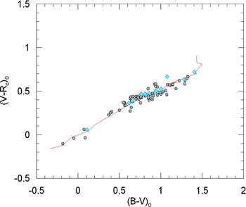
Figure 3. (B − V)0 × (V − Rc )0 two-colour diagram of the sample stars. The positions of 15 stars with synthetic (B − V)0 and (V − Rc )0 colours are marked with a different symbol (⋄). The solid line indicates the synthetic two-colour diagram of Pickles (Reference Pickles1998).

Figure 4. (g′ − r′)0 × (r′ − i′)0 two-colour diagram of the sample stars. The solid line indicates the synthetic two-colour diagram of Covey et al. (Reference Covey2007).

Figure 5. Distributions of the errors of the magnitudes and colours of the sample stars.
3 TRANSFORMATIONS
The following general equations have been preferred to derive the 18 sets of transformation equations with their coefficients between BVRc and g′r′i′ photometric systems using de-reddened magnitudes and colours of the sample giants in this study. Equations (9)–(17) transform BVRc into g′r′i′ magnitudes and colours, while Equations (18)–(26) are their inverse transformations. The equations are:
 \begin{eqnarray}
(g^{\prime }-V)_{0}=a_{i}(B-V)_{0}^2+b_{i}(B-V)_{0}+c_{i}
\end{eqnarray}
\begin{eqnarray}
(g^{\prime }-V)_{0}=a_{i}(B-V)_{0}^2+b_{i}(B-V)_{0}+c_{i}
\end{eqnarray}
 \begin{eqnarray}
(g^{\prime }-V)_{0}=a_{i}(V-R_c)_{0}^2+b_{i}(V-R_c)_{0}+c_{i}
\end{eqnarray}
\begin{eqnarray}
(g^{\prime }-V)_{0}=a_{i}(V-R_c)_{0}^2+b_{i}(V-R_c)_{0}+c_{i}
\end{eqnarray}
 \begin{eqnarray}
(g^{\prime }-V)_{0}=a_{i}(B-V)_{0}+b_{i}(V-R_c)_{0}+c_{i}
\end{eqnarray}
\begin{eqnarray}
(g^{\prime }-V)_{0}=a_{i}(B-V)_{0}+b_{i}(V-R_c)_{0}+c_{i}
\end{eqnarray}
 \begin{eqnarray}
(g^{\prime }-r^{\prime })_{0}=a_{i}(B-V)_{0}^2+b_{i}(B-V)_{0}+c_{i}
\end{eqnarray}
\begin{eqnarray}
(g^{\prime }-r^{\prime })_{0}=a_{i}(B-V)_{0}^2+b_{i}(B-V)_{0}+c_{i}
\end{eqnarray}
 \begin{eqnarray}
(g^{\prime }-r^{\prime })_{0}=a_{i}(V-R_c)_{0}^2+b_{i}(V-R_c)_{0}+c_{i}
\end{eqnarray}
\begin{eqnarray}
(g^{\prime }-r^{\prime })_{0}=a_{i}(V-R_c)_{0}^2+b_{i}(V-R_c)_{0}+c_{i}
\end{eqnarray}
 \begin{eqnarray}
(g^{\prime }-r^{\prime })_{0}=a_{i}(B-V)_{0}+b_{i}(V-R_c)_{0}+c_{i}
\end{eqnarray}
\begin{eqnarray}
(g^{\prime }-r^{\prime })_{0}=a_{i}(B-V)_{0}+b_{i}(V-R_c)_{0}+c_{i}
\end{eqnarray}
 \begin{eqnarray}
(r^{\prime }-i^{\prime })_{0}=a_{i}(B-V)_{0}^2+b_{i}(B-V)_{0}+c_{i}
\end{eqnarray}
\begin{eqnarray}
(r^{\prime }-i^{\prime })_{0}=a_{i}(B-V)_{0}^2+b_{i}(B-V)_{0}+c_{i}
\end{eqnarray}
 \begin{eqnarray}
(r^{\prime }-i^{\prime })_{0}=a_{i}(V-R_c)_{0}^2+b_{i}(V-R_c)_{0}+c_{i}
\end{eqnarray}
\begin{eqnarray}
(r^{\prime }-i^{\prime })_{0}=a_{i}(V-R_c)_{0}^2+b_{i}(V-R_c)_{0}+c_{i}
\end{eqnarray}
 \begin{eqnarray}
(r^{\prime }-i^{\prime })_{0}=a_{i}(B-V)_{0}+b_{i}(V-R_c)_{0}+c_{i}
\end{eqnarray}
\begin{eqnarray}
(r^{\prime }-i^{\prime })_{0}=a_{i}(B-V)_{0}+b_{i}(V-R_c)_{0}+c_{i}
\end{eqnarray}
 \begin{eqnarray}
(V-g^{\prime })_{0}=d_{i}(g^{\prime }-r^{\prime })_{0}^2+e_{i}(g^{\prime }-r^{\prime })_{0}+f_{i}
\end{eqnarray}
\begin{eqnarray}
(V-g^{\prime })_{0}=d_{i}(g^{\prime }-r^{\prime })_{0}^2+e_{i}(g^{\prime }-r^{\prime })_{0}+f_{i}
\end{eqnarray}
 \begin{eqnarray}
(V-g^{\prime })_{0}=d_{i}(r^{\prime }-i^{\prime })_{0}^2+e_{i}(r^{\prime }-i^{\prime })_{0}+f_{i}
\end{eqnarray}
\begin{eqnarray}
(V-g^{\prime })_{0}=d_{i}(r^{\prime }-i^{\prime })_{0}^2+e_{i}(r^{\prime }-i^{\prime })_{0}+f_{i}
\end{eqnarray}
 \begin{eqnarray}
(V-g^{\prime })_{0}=d_{i}(g^{\prime }-r^{\prime })_{0}+e_{i}(r^{\prime }-i^{\prime })_{0}+f_{i}
\end{eqnarray}
\begin{eqnarray}
(V-g^{\prime })_{0}=d_{i}(g^{\prime }-r^{\prime })_{0}+e_{i}(r^{\prime }-i^{\prime })_{0}+f_{i}
\end{eqnarray}
 \begin{eqnarray}
(B-V)_{0}=d_{i}(g^{\prime }-r^{\prime })_{0}^2+e_{i}(g^{\prime }-r^{\prime })_{0}+f_{i}
\end{eqnarray}
\begin{eqnarray}
(B-V)_{0}=d_{i}(g^{\prime }-r^{\prime })_{0}^2+e_{i}(g^{\prime }-r^{\prime })_{0}+f_{i}
\end{eqnarray}
 \begin{eqnarray}
(B-V)_{0}=d_{i}(r^{\prime }-i^{\prime })_{0}^2+e_{i}(r^{\prime }-i^{\prime })_{0}+f_{i}
\end{eqnarray}
\begin{eqnarray}
(B-V)_{0}=d_{i}(r^{\prime }-i^{\prime })_{0}^2+e_{i}(r^{\prime }-i^{\prime })_{0}+f_{i}
\end{eqnarray}
 \begin{eqnarray}
(B-V)_{0}=d_{i}(g^{\prime }-r^{\prime })_{0}+e_{i}(r^{\prime }-i^{\prime })_{0}+f_{i}
\end{eqnarray}
\begin{eqnarray}
(B-V)_{0}=d_{i}(g^{\prime }-r^{\prime })_{0}+e_{i}(r^{\prime }-i^{\prime })_{0}+f_{i}
\end{eqnarray}
 \begin{eqnarray}
(V-R_c)_{0}=d_{i}(g^{\prime }-r^{\prime })_{0}^2+e_{i}(g^{\prime }-r^{\prime })_{0}+f_{i}
\end{eqnarray}
\begin{eqnarray}
(V-R_c)_{0}=d_{i}(g^{\prime }-r^{\prime })_{0}^2+e_{i}(g^{\prime }-r^{\prime })_{0}+f_{i}
\end{eqnarray}
 \begin{eqnarray}
(V-R_c)_{0}=d_{i}(r^{\prime }-i^{\prime })_{0}^2+e_{i}(r^{\prime }-i^{\prime })_{0}+f_{i}
\end{eqnarray}
\begin{eqnarray}
(V-R_c)_{0}=d_{i}(r^{\prime }-i^{\prime })_{0}^2+e_{i}(r^{\prime }-i^{\prime })_{0}+f_{i}
\end{eqnarray}
 \begin{eqnarray}
(V-R_c)_{0}=d_{i}(g^{\prime }-r^{\prime })_{0}+e_{i}(r^{\prime }-i^{\prime })_{0}+f_{i}.\\
\nonumber
\end{eqnarray}
\begin{eqnarray}
(V-R_c)_{0}=d_{i}(g^{\prime }-r^{\prime })_{0}+e_{i}(r^{\prime }-i^{\prime })_{0}+f_{i}.\\
\nonumber
\end{eqnarray}
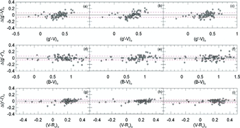
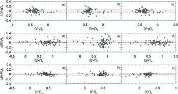
The values of the coefficients and their errors are given in Tables 6 and 7. The distribution of the sample stars on the colour planes are plotted in Figure 6. The ranges of the magnitudes and colours in the transformations are: 7.10 < V 0 < 14.50, 7.30 < g 0 < 14.85, − 0.20 < (B − V)0 < 1.41, − 0.11 < (V − Rc )0 < 0.73, − 0.42 < (g − r)0 < 1.15, and − 0.37 < (r − i)0 < 0.47 mag. The residuals of the colours from the curve fits are plotted in Figures 7 and 8, while the means and standard deviations of the residuals are included to the data in Tables 6 and 7.
Table 6. Coefficients for the Equations (9)–(17). The figures in the first line indicate the equation number, R is the correlation coefficient and, s and m.r. are the standard deviation, and mean residuals, respectively.

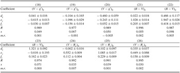
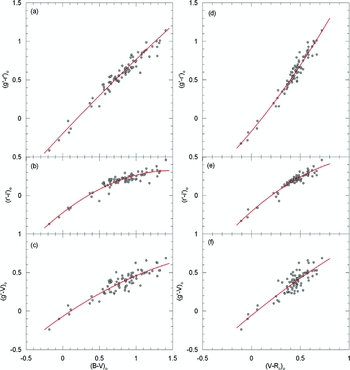
Figure 6. Distributions of the sample stars in six colour planes. The curves indicate quadratic polynomials.


The transformation equations from BVRc to g′r′i′ colours derived in this study have been applied to another sample of 427 giants taken from Pickles & Depagne (Reference Pickles and Depagne2010) as explained in the following. Smith et al. (Reference Smith2005) have published a list of ~ 16000 southern SDSS standards, which includes some repetition. 6117 of them were turned out to be of luminosity class III, i.e. giants, which cover the spectral range A-M. We have selected a sample of 427 giants with uncertainties in g′, r′ and i′ less than 0.01 mag. The E(B − V) colour excesses used for de-reddening the g′ magnitudes, and g′ − r′ and r′ − i′ colours have been evaluated in two steps, by a procedure similar to the one used for the original sample from which the Equations (7) and (8) derived as in Section 2.2. The g′ magnitudes, and g′ − r′ and r′ − i′ colours are de-reddened according to the corresponding E(B − V) colour excesses of the stars and the equations of Fan (Reference Fan1999). The (g′ − r′)0 × (r′ − i′)0 two-colour diagram of the sample of 427 stars obtained from Pickles & Depagne (Reference Pickles and Depagne2010) are given in Figure 9.

Figure 9. (g′ − r′)0 × (r′ − i′)0 two-colour diagram of 427 stars used for the application of the transformation equations. The solid line indicates the synthetic two-colour diagram of Covey et al. (Reference Covey2007).
To estimate intrinsic BVRc colours of the sample of those 427 giants, we have identified them first in Pickles & Depagne (Reference Pickles and Depagne2010), and then recorded their V magnitudes and, B − V and V − Rc colours. Then, those V magnitudes and, B − V and V − Rc colours are de-reddened by the procedure explained in the Section 2.2, and transformed them to g′0 magnitudes and, (g′ − r′)0 and (r′ − i′)0 colours by using the transformation equations derived from the original sample of 80 giants in this study. Then, we have compared those g′0 magnitude and, (g′ − r′)0 and (r′ − i′)0 colours obtained through transformation equations to the g′0 magnitude and, (g′ − r′)0 and (r′ − i′)0 colours evaluated from Pickles & Depagne (Reference Pickles and Depagne2010). The residuals, i.e. the differences between the original and evaluated colours, are plotted in Figure 10. The mean and standard deviations of the residuals for each colour are also indicated in the corresponding panel of the figure.

Figure 10. Distributions of the residuals of 427 stars used for the application of the transformation equations. Mean residuals (m.r.) and standard deviations (s) are also indicated in each panel.
4 SUMMARY AND DISCUSSION
The transformation equations from BVRc to g′r′i′ colours and vice versa for giants were derived and presented. The transformation equations were obtained using the observed magnitudes and colours of a sample of 80 giants selected from the Pastel catalogue (Soubiran et al. Reference Soubiran, Le Campion, de Strobel and Caillo2010) with confirmed surface gravity (2 ⩽ logg (cms− 2) ⩽ 3) at effective temperatures from 4000 to 16000 K. The g′r′i′ magnitudes of all sample and 65 of them at BVRc magnitudes were obtained by observations carried out with the T100 telescope at TUG at Bakırlıtepe, Antalya, in the years 2011–2012. The BVRc magnitudes of 15 giants were completed from the synthetic BVRc magnitudes in Pickles & Depagne (Reference Pickles and Depagne2010). We have used the MV absolute magnitudes and Teff temperatures for giants at various spectral types presented in Sung et al. (Reference Sung, Lim, Bessell, Kim, Hur, Chun and Park2013) to produce Figure 1, which were used to estimated the MV absolute magnitudes of the sample stars used in this study. We have de-reddened the magnitude and colours in both photometric systems, BVRc and g′r′i′ of the sample by a procedure commonly used in the literature.
The transformation equations from BVRc to g′r′i′ (Equations (9)–(17)) and inverse transformations (Equations (18)–(26)) were derived by fitting quadratic polynomials to (g′ − V)0, (g′ − r′)0 and (r′ − i′)0 which are given in terms of (B − V)0 only or (V − Rc )0 only, or by fitting a linear function to them if they are expressed both (B − V)0 and (V − Rc )0. Similarly, (V − g′)0, (B − V)0 and (V − Rc )0 expressed by a quadratic function of (g′ − r′)0 or (r′ − i′)0, or they are expressed by a linear function fit both (g′ − r′)0 and (r′ − i′)0 colours used in the equation. The correlation coefficients and the standard deviations in Table 6 show that all the transformation Equations (9)–(17) provide sufficiently accurate magnitude and colours. However, the most accurate colours (g′ − V)0, (g′ − r′)0 and (r′ − i′)0 come from the quadratic equations containing only (B − V)0, or (V − Rc )0. The correlation coefficients given in Table 7 for inverse transformations are a bit larger, while the standard deviations are smaller. The most accurate colours (V − g′)0, (B − V)0, and (V − Rc )0 come from the quadratic equations containing only (g′ − r′)0, or (r′ − i′)0 and from the linear equation if both (g′ − r′)0 and (r′ − i′)0 appear in the equation.
The transformation equations could be considered valid for the ranges of the magnitudes and colours used in the transformations: 7.10 < V 0 < 14.50, 7.30 < g′0 < 14.85, − 0.20 < (B − V)0 < 1.41, − 0.11 < (V − Rc )0 < 0.73, − 0.42 < (g′ − r′)0 < 1.15, and − 0.37 < (r′ − i′)0 < 0.47 mag, rather larger than the ones provided by Yaz et al. (Reference Yaz, Bilir, Karaali, Ak, Coşkunoğlu and Cabrera-Lavers2010), i.e. 0.25 < (B − V)0 < 1.35, 0.10 < (g − r)0 < 0.95, and 0 < (r − i)0 < 0.35.
We applied the transformation equations derived in this study to the synthetic BVRc data of 427 giants taken from Pickles & Depagne (Reference Pickles and Depagne2010). The ranges of the mean residuals (m.r.) and standard deviations (s) are − 0.010 ⩽ m.r. ⩽ 0.042 and 0.028 ⩽ s ⩽ 0.068 mag, respectively. That is, the g′ magnitude and, (g′ − r′)0 and (r′ − i′)0 colours of a giant can be estimated by our transformations with an accuracy of at least ~ 0.05 mag. Yaz et al. (Reference Yaz, Bilir, Karaali, Ak, Coşkunoğlu and Cabrera-Lavers2010) derived transformations between 2MASS, SDSS and BVI photometric systems for late type giants for two cases, i.e. metallicity dependent and free of metallicity. We have compared their residuals and the standard deviations free of metallicity. Their mean residuals are rather small, i.e. − 0.0005 ⩽ m.r. ⩽ 0.0004 mag. However, the corresponding standard deviations are larger than the ones in our study, 0.075 ⩽ s ⩽ 0.167 mag. That is, our study provides magnitudes and colours with an accuracy of ~ 1.5 times that of Yaz et al. (Reference Yaz, Bilir, Karaali, Ak, Coşkunoğlu and Cabrera-Lavers2010).
Sufficiently small residuals and the standard deviations confirm the quality of the observations made in TUG, and accuracy and the precision of the reductions applied to these observations. The metallicities of the sample stars used for deriving the coefficents of the transformation equations between the two photometric systems cover a large range, − 4 ⩽ [Fe/H] ⩽ 0.5 dex. However, the number of stars with [Fe/H] < −1 dex are small. Hence, we did not consider the metallicity in our transformations. Though, we obtained transformation equations which provide accurate colour and magnitudes.
ACKNOWLEDGMENTS
This work has been supported in part by the Scientific and Technological Research Council (TÜBİTAK) 212T214.
We thank to TÜBİTAK for a partial support in using T100 telescope with project number 11BT100-184-2.
This research has made use of the NASA/IPAC Infrared Science Archive and Extragalactic Database (NED) which are operated by the Jet Propulsion Laboratory, California Institute of Technology, under contract with the National Aeronautics and Space Administration.
This research has made use of the SIMBAD, and NASA's Astrophysics Data System Bibliographic Services.