


1 INTRODUCTION
Analysis of stellar binary systems is the most reliable and accurate way of estimating stellar physical and geometrical parameters, especially stellar masses. It emphasises the role of binary stars in examining some physical and stellar evolutionary theories. Even high resolution observational techniques, like speckle interferometry and adaptive optics, are not sufficient to determine the physical parameters of the individual components of visually close (spatially unresolved on the sky) binary systems (VCBS), especially in the case of this study (HD25811) which has no parallax measurement.
Combining spectrophotometry with atmospheric modelling gives a new method for the accurate determination of the physical and geometrical parameters of both components of VCBS, in addition to the estimation of their spectral types, luminosity classes, and ages. This method, first advised by Al-Wardat (Reference Al-Wardat2002a, Reference Al-Wardat2007), was applied to several VCBS such as ADS11061, Cou1289, Cou1291, Hip11352, Hip11253, Hip70973, and Hip72479 (Al-Wardat Reference Al-Wardat2002a, Reference Al-Wardat2007, Reference Al-Wardat2009, Reference Al-Wardat2012; Al-Wardat & Widyan Reference Al-Wardat and Widyan2009).
In this paper, we are developing the method by combining the dynamical analysis of the relative orbit of the binary, a step which will strengthen the method, reduce the error bars, and make it applicable to evolved binaries by accurate determination of the individual masses.
The system HD25811 (SAO 93759 = CHA13 = BAG 4) was first resolved as a binary using the lunar-occultation observational technique in the early eighties (Schmidtke & Africano Reference Schmidtke and Africano1984; Evans et al. Reference Evans, Edwards, Frueh, McWilliam and Sandmann1985). Subsequently, it was included in the speckle interferometric programme of the Russian 6-metre telescope by Balega & Balega (Reference Balega and Balega1987), and was designated as BAG 4. Since then it is routinely observed by speckle interferometric techniques all over the world to achieve as much data as possible in order to calculate its best orbit (McAlister et al. Reference McAlister, Hartkopf, Hutter and Franz1987; Balega, Balega, & Vasyuk Reference Balega, Balega and Vasyuk1989; McAlister et al. Reference McAlister, Hartkopf, Sowell, Dombrowski and Franz1989, Reference McAlister, Hartkopf and Franz1990; Hartkopf, McAlister, & Franz Reference Hartkopf, McAlister and Franz1992; Bagnuolo et al. Reference Bagnuolo, Mason, Barry, Hartkopf and McAlister1992; Balega et al. Reference Balega, Balega, Belkin, Maximov, Orlov, Pluzhnik, Shkhagosheva and Vasyuk1994, Reference Balega, Balega, Hofmann and Weigelt2001, Reference Balega, Balega, Maksimov, Malogolovets, Rastegaev, Shkhagosheva and Weigelt2007)(see Table 1). But it was not listed in the Hipparcos programme, which is why it has no trigonometric parallax measurement.
Table 1. Relative positional measurements using different methods which are used to build the orbit of the system. These points are taken from the Fourth Catalog of Interferometric Measurements of Binary Stars and a point from Al-Wardat (Reference Al-Wardat2003).
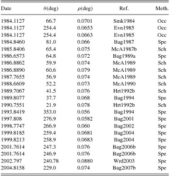
Note: Occ = occultaion; Spe = speckle interferometry; Sch = CHARA speckle; Wrd2003 = Al-Wardat (Reference Al-Wardat2003). References are abbreviated as in the Fourth Catalog of Interferometric Measurements of Binary Stars.
The VCBS HD25811 (BAG 4) fulfils the requirements of the aforementioned method, where it has precise magnitude difference measurements and observational spectral energy distribution (SED) covers the optical range. It has also several relative positional measurements listed in the Fourth Catalog of Interferometric Measurements of Binary Stars (http://ad.usno.navy.mil/wds/int4.html), which they used to build its preliminary orbit and a new positional measurement that can be used to modify it.
In addition to that, HD26811 represents a very good example for studying the formation and evolution of stellar binary systems, since, as we shall prove, it consists of two subgiant stars.
Table 2 contains the basic data of the system from SIMBAD and other databases, and Table 3 contains data from Tycho-2 Catalogue (ESA 1997).
Table 2. Data from SIMBAD and NASA/IPAC.
Note: 1 = SIMBAD; 2 = NASA/IPAC:http://irsa.ipac.caltech.edu
Table 3. Data from Tycho-2 catalogue (Høg et al. Reference Høg2000).
2 ORBITAL ELEMENTS
The orbit of the system was calculated firstly by Balega et al. (Reference Balega, Balega, Hofmann and Weigelt2001) using the first 15 relative positional measurements in Table 1, they noted that they will have to wait another ~10 years to obtain a reliable solution. Then it was modified by Al-Wardat (Reference Al-Wardat2003) using the measurements up to 2002.797. A new slight modification of the orbit is introduced here using all relative positional measurements listed in Table 1, which cover around 210° of the complete orbit.
The estimated orbital parameters of the system along with those of the old orbits are listed in Table 4.
Table 4. Estimated orbital elements of the system with those of the old orbits by Balega et al. (Reference Balega, Balega, Hofmann and Weigelt2001) and Al-Wardat (Reference Al-Wardat2003).
Figure 1 shows the relative visual orbit of the system with the epoch of the positional measurements, and Figure 2 shows the new orbit against the old orbits of Balega et al. (Reference Balega, Balega, Hofmann and Weigelt2001) and Al-Wardat (Reference Al-Wardat2003).
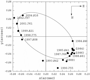
Figure 1. Relative visual orbit of the system with the epoch of the positional measurements; the origin represents the position of the primary component.
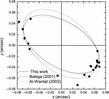
Figure 2. Comparison between the modified relative visual orbit of the system in this work (solid line) and those of Balega et al. (Reference Balega, Balega, Hofmann and Weigelt2001) (dashed line) and Al-Wardat (Reference Al-Wardat2003) (doted line).
Unfortunately, there is no any positional measurement for the system during the last 9 years, which would have covered the whole orbital period. This could give a more reliable orbit and hence more precise geometrical parameters.
3 ATMOSPHERIC MODELLING
To calculate the individual components’ preliminary input parameters (T eff and log g), we followed the procedures explained in Al-Wardat (Reference Al-Wardat2012) using the following relations (e.g., Lang Reference Lang and Lang1992; Gray Reference Gray and Gray2005):
 \begin{eqnarray}
m_v=-2.5\log (f_1+f_2)
\end{eqnarray}
\begin{eqnarray}
m_v=-2.5\log (f_1+f_2)
\end{eqnarray}
 \begin{eqnarray}
M_v=m_v+5-5\log (d)-A,
\end{eqnarray}
\begin{eqnarray}
M_v=m_v+5-5\log (d)-A,
\end{eqnarray}
 \begin{eqnarray}
\log (R/R_\odot )= 0.5 \log (L/L_\odot )-2\log (T/T_\odot ),
\end{eqnarray}
\begin{eqnarray}
\log (R/R_\odot )= 0.5 \log (L/L_\odot )-2\log (T/T_\odot ),
\end{eqnarray}
 \begin{eqnarray}
\log g = \log (M/M_\odot )- 2\log (R/R_\odot ) + 4.43,
\end{eqnarray}
\begin{eqnarray}
\log g = \log (M/M_\odot )- 2\log (R/R_\odot ) + 4.43,
\end{eqnarray}
So, using the entire visual magnitude of the system mv
= 8.m66 from Table 3 and ▵m = 0.m23 from speckle interferometric results (Table 5) as the average of ▵m measurement under the filter 545nm/30 (the closest filter to the Johnson V filter), we got $m_{v\rm a}=9\hbox{$.\!\!^m$}304$
and
$m_{v\rm a}=9\hbox{$.\!\!^m$}304$
and $m_{v\rm b}=9\hbox{$.\!\!^m$}534$
.
$m_{v\rm b}=9\hbox{$.\!\!^m$}534$
.
Table 5. Magnitude difference between the components of the system, along with the filter used to obtain the observations.
Note: 1 = Balega et al. (Reference Balega, Balega, Hofmann, Maksimov, Pluzhnik, Schertl, Shkhagosheva and Weigelt2002); 2 = Balega et al. (Reference Balega, Balega, Maksimov, Pluzhnik, Schertl, Shkhagosheva and Weigelt2004); 3 = Balega et al. (Reference Balega, Balega, Maksimov, Malogolovets, Pluzhnik and Shkhagosheva2006); 4 = Balega et al. (Reference Balega, Balega, Maksimov, Malogolovets, Rastegaev, Shkhagosheva and Weigelt2007).
The dynamical parallax estimated by Al-Wardat (Reference Al-Wardat2003)(π = 5.24 ± 0.6, d = 191 pc) is used as a preliminary value to calculate the individual absolute magnitudes according to the following equation:
 \begin{eqnarray}
M_v=m_v+5-5\log (d)-A.
\end{eqnarray}
\begin{eqnarray}
M_v=m_v+5-5\log (d)-A.
\end{eqnarray}
This leads to the following preliminary input parameters:
 \begin{eqnarray}
M_{v\rm a}=2\hbox{$.\!\!^m$}03, \,\,\,\, M_{v\rm b}=2\hbox{$.\!\!^m$}26
\end{eqnarray}
\begin{eqnarray}
M_{v\rm a}=2\hbox{$.\!\!^m$}03, \,\,\,\, M_{v\rm b}=2\hbox{$.\!\!^m$}26
\end{eqnarray}
 \begin{eqnarray}
T_{\rm eff}^{\rm a}=8150\,{\rm K}, \,\, \, T_{\rm eff}^{\rm b}=7950\,{\rm K},
\end{eqnarray}
\begin{eqnarray}
T_{\rm eff}^{\rm a}=8150\,{\rm K}, \,\, \, T_{\rm eff}^{\rm b}=7950\,{\rm K},
\end{eqnarray}
 \begin{eqnarray}
\log \,g_{\rm a}=4.2, \,\,\, \log \,g_{\rm b}=4.2,
\end{eqnarray}
\begin{eqnarray}
\log \,g_{\rm a}=4.2, \,\,\, \log \,g_{\rm b}=4.2,
\end{eqnarray}
3.1 Synthetic spectra
The observational SED of the entire system was taken from Al-Wardat (Reference Al-Wardat2002b) (Figure 3). It shows some strong lines and depressions, especially in the red part of the spectrum (around λ6867Å, λ7200Å, and λ7605Å). These are H2O and O2 telluric lines and depressions. Synthetic Jonson-Cousins, Strömgren, and Tycho magnitudes and colour indices of this observational SED are listed in Table 6.
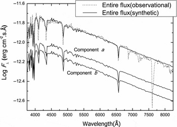
Figure 3. Dotted line: observational SED in the continuous spectrum of the system. Solid lines: the entire computed SED of the two components, the computed flux of the primary component with T eff = 6850 ± 50 K, log g = 4.04 ± 0.10, R = 1.96 ± 0.20R ⊙, and the computed flux of the secondary component with T eff = 7000 ± 50 K, log g = 4.15 ± 0.10, R = 1.69 ± 0.20R ⊙, and d = 196.27 pc.
Table 6. Entire synthetic Johnson-Cousins, Strömgren, and Tycho magnitudes and colour indices of the system HD25811 (Al-Wardat Reference Al-Wardat2008).
Synthetic SEDs of the individual components are built first using solar metalicity model atmospheres as the output of ATLAS 9 of the preliminary parameters (Equs. 6, 7, and 8), R a = 1.55 R⊙, R b = 1.45 R⊙, and d = 191pc (from Al-Wardat Reference Al-Wardat2003). The total energy flux from a binary star is created from the net luminosities of the components a and b located at a distance d from the Earth as follows:
 \begin{equation}
F_{\lambda } \cdot d^2 = H_{\lambda }^{\rm a} \cdot R_{\rm a}^2 + H_{\lambda }^{\rm b} \cdot R_{\rm b}^2\,,
\end{equation}
\begin{equation}
F_{\lambda } \cdot d^2 = H_{\lambda }^{\rm a} \cdot R_{\rm a}^2 + H_{\lambda }^{\rm b} \cdot R_{\rm b}^2\,,
\end{equation}
 \begin{equation}
F_{\lambda } = (R_{\rm a}^2/d)^2(H_{\lambda }^{\rm a} + H_{\lambda }^{\rm b} \cdot (R_{\rm b}/R_{\rm a})^2)\,,
\end{equation}
\begin{equation}
F_{\lambda } = (R_{\rm a}^2/d)^2(H_{\lambda }^{\rm a} + H_{\lambda }^{\rm b} \cdot (R_{\rm b}/R_{\rm a})^2)\,,
\end{equation}
The resultant entire synthetic SED did not fit the observational SED. Therefore, many attempts were made and hundreds of synthetic SEDs were built, using different sets of parameters, and compared with the observational SED to achieve the best fit. The attempts included changing the effective temperatures, gravity acceleration, parallax, and radii. It is worthwhile mentioning that the step size of the change was less than or equal to the estimated error in each parameter. In the case of the effective temperatures and radii, the changes exceed the errors of the first estimations because we are dealing with subgiants instead of main sequence, or in other words, that is what we discovered.
Kepler's equation is used to match between the physical and geometrical parameters, and to connect the dynamical analysis with the atmospheric modelling:
 \begin{eqnarray}
\ \left(\frac{M_a + M_b}{M_\odot }\right)(\pi ^3)=\frac{a^3}{p^2},
\end{eqnarray}
\begin{eqnarray}
\ \left(\frac{M_a + M_b}{M_\odot }\right)(\pi ^3)=\frac{a^3}{p^2},
\end{eqnarray} $(\frac{M_a + M_b}{M_\odot })$
is the mass sum of the two components in terms of solar mass, π is the parallax of the system in arc seconds, a is the semi-major axes in arc seconds, and p is the period in years.
$(\frac{M_a + M_b}{M_\odot })$
is the mass sum of the two components in terms of solar mass, π is the parallax of the system in arc seconds, a is the semi-major axes in arc seconds, and p is the period in years.
Fixing the right part of Equation (11) according to the orbital elements of the system calculated in Section 2, and changing the values of the left part in an iterated way, ensures agreement between the masses of the components, their positions on the evolutionary tracks, and the best fit between the synthetic and observational SEDs.
For stars with formerly estimated temperatures, masses, and gravity accelerations, this agreement is possible only for radii bigger than what would be if they were main sequence stars (the preliminary input radii), which means that both components are evolved subgiant stars.
Within the criteria of the best fit, which are the maximum values of the absolute fluxes, the inclination of the continuum of the spectra, and the profiles of the absorption lines, the best fit (Figure 3) is found using the following set of parameters:
 \begin{equation}
T_{\rm eff}^{\rm a} =6850\pm 50\,{\rm K}, \ T_{\rm eff}^{\rm b} =7000\pm 50\,{\rm K},
\end{equation}
\begin{equation}
T_{\rm eff}^{\rm a} =6850\pm 50\,{\rm K}, \ T_{\rm eff}^{\rm b} =7000\pm 50\,{\rm K},
\end{equation}
 \begin{equation}
\log g_{\rm a}=4.04\pm 0.10, \ \log g_{\rm b}=4.15\pm 0.10,
\end{equation}
\begin{equation}
\log g_{\rm a}=4.04\pm 0.10, \ \log g_{\rm b}=4.15\pm 0.10,
\end{equation}
 \begin{equation}
R_{\rm a}=1.96\pm 0.20\,{\rm R}_{\odot }, R_{\rm b}=1.69\pm 0.20\,{\rm R}_{\odot },
\end{equation}
\begin{equation}
R_{\rm a}=1.96\pm 0.20\,{\rm R}_{\odot }, R_{\rm b}=1.69\pm 0.20\,{\rm R}_{\odot },
\end{equation}
 \begin{equation}
(M_a + M_b)/M_\odot = 3.05\pm 0.10,
\end{equation}
\begin{equation}
(M_a + M_b)/M_\odot = 3.05\pm 0.10,
\end{equation}
The role of Equation (11) rises here to assure the compatibility between the parallax of the system and its mass sum being given the period and the semi-major axes.
The complete set of the physical and geometrical parameters are listed in Table 7.
Table 7. Physical and geometrical parameters of the system HD25811 components.
The estimated parameters are highly dependent on the precision of observations. Thus, within the error values of the measured quantities, they represent adequately enough the parameters of the systems’ components.
Depending on the tables of Straizys & Kuriliene (Reference Straizys and Kuriliene1981) and Gray (Reference Gray and Gray2005), the spectral types for the components of the system are estimated as F2 IV for the primary component and F1 IV for the secondary component.
4 SYNTHETIC PHOTOMETRY
In addition to its importance in calculating the entire and individual synthetic magnitudes of the system, synthetic photometry is used here as an evaluation technique to examine the best fit between the synthetic and observational spectra. This is performed by comparing the observed magnitudes of the entire system from different sources with the entire synthetic ones using the following relation Maíz Apellániz (Reference Maíz Apellániz2006) and Maíz Apellániz (Reference Maíz Apellániz and Sterken2007):
 \begin{equation}
m_p[F_{\lambda ,s}(\lambda )] = -2.5 \log \frac{\int P_{p}(\lambda )F_{\lambda ,s}(\lambda )\lambda {\rm d}\lambda }{\int P_{p}(\lambda )F_{\lambda ,r}(\lambda )\lambda {\rm d}\lambda }+ {\rm ZP}_p\,,
\end{equation}
\begin{equation}
m_p[F_{\lambda ,s}(\lambda )] = -2.5 \log \frac{\int P_{p}(\lambda )F_{\lambda ,s}(\lambda )\lambda {\rm d}\lambda }{\int P_{p}(\lambda )F_{\lambda ,r}(\lambda )\lambda {\rm d}\lambda }+ {\rm ZP}_p\,,
\end{equation}
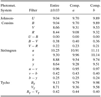
Table 8 shows the magnitudes and colour indices of the entire system and individual components in UBVR Johnson-Cousins, uvby Strömgren, and BV Tycho.
Table 8. Synthetic magnitudes and colour indices of the system.
5 RESULTS AND DISCUSSION
Comparing the synthetic magnitudes and colours with the observational ones (Table 9) shows a high consistency between them. This gives a good indication about the reliability of the estimated parameters of the individual components of the system which are listed in Table 7.
Table 9. Comparison between the observational and synthetic magnitudes, colours, and magnitude differences of the system.
Figure 4 shows the positions of the system's components on the evolutionary tracks of Girardi et al. (Reference Girardi, Bressan, Bertelli and Chiosi2000). It shows that the primary more massive component is more evolved than the secondary, which is why the estimated value of the luminosity of the primary is greater than the expected value for an MS star of the same mass.
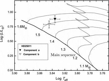
Figure 4. Components of the system on the evolutionary tracks of Girardi et al. (Reference Girardi, Bressan, Bertelli and Chiosi2000).
The estimated parameters of the system (Table 7) show that the components of the system are similar to the star β Hydri (HIP 2021), which is a G2IV evolved subgiant with an age of about 6.5–7.0 Gyr (Dravins, Lindegren, & Vandenberg Reference Dravins, Lindegren and Vandenberg1998; Fernandes & Monteiro Reference Fernandes and Monteiro2003), $\overline{\rho }(\overline{\rho }_\odot )=0.1803\pm 0.0011$
(Bedding et al. (Reference Bedding2007) using high precision asteroseismology) and T
eff(K) = 5872 ± 44,
$\overline{\rho }(\overline{\rho }_\odot )=0.1803\pm 0.0011$
(Bedding et al. (Reference Bedding2007) using high precision asteroseismology) and T
eff(K) = 5872 ± 44, $R(\textrm {R}_{\odot }=1.814\pm 0.017$
), log g = 3.952 ± 0.005
$R(\textrm {R}_{\odot }=1.814\pm 0.017$
), log g = 3.952 ± 0.005 $L (\textrm {L}_\odot )=3.51\pm 0.09$
and mass
$L (\textrm {L}_\odot )=3.51\pm 0.09$
and mass $M (\textrm {M}_{\odot })= 1.07\pm 0.03$
(North et al. (Reference North2007) using interferometry).
$M (\textrm {M}_{\odot })= 1.07\pm 0.03$
(North et al. (Reference North2007) using interferometry).
This, in addition to their luminosity-temperature relation which reflects their positions on the HR diagram and the evolutionary tracks (see Figure 4), their absolute magnitudes which are brighter than those of MS stars of the same temperatures, and their densities, leads us to conclude that both components are subgiant stars.
The age of the system was established from the evolutionary tracks as almost 2 Gy. The similarity between the two components leads us to adopt the fragmentation process for the formation of the system, since it is the most likely mechanism in this case (for more discussion, see Bonnell Reference Bonnell, Zinnecker and Mathieu2001; Fabian, Pringle, & Rees Reference Fabian, Pringle and Rees1975; Binney & Tremaine Reference Binney, Tremaine, Binney and Tremaine1987).
6 CONCLUSIONS
The VCBS HD25811 is analysed using a modified version of the complex method which was first advised by Al-Wardat (Reference Al-Wardat2002a, Reference Al-Wardat2007).
The modification in the method includes the dynamical analysis of the relative orbit of the system (which is very helpful in the determination of the masses of the individual components of the system) and consequently their spectral types, by combining them with the atmospheric modelling input parameters.
The physical and geometrical parameters of the system's components are estimated depending on the best fit between the observational and synthetic SEDs, built using the atmospheric modelling of the individual components and the system's orbital elements.
Both components of the system are concluded to be F2 IV for the primary and F1 IV for the secondary.
The entire and individual UBVR Johnson-Cousins, uvby Strömgren, and BV Tycho synthetic magnitudes and colours of the system are calculated.
Finally, fragmentation was proposed as the most likely process for the formation and evolution of the system.
ACKNOWLEDGEMENTS
This work made use of the Fourth Interferometric Catalogue, SIMBAD database, and CHORIZOS code of photometric and spectrophotometric data analysis (http://www.stsci.edu/jmaiz/software/chorizos/chorizos.html). The authors thank Miss. Kawther Al-Waqfi for her help in some calculations and Mrs. Donna Keeley for the language editing.


