INTRODUCTION
Haemorrhagic fever with renal syndrome (HFRS) is a zoonotic disease with fever, haemorrhage, headache, back pain, abdominal pain, and acute kidney injury. The disease is caused by hantaviruses [Reference Clement1] and is an important public health problem in the People's Republic of China with about 20 000–50 000 human cases reported annually, accounting for 90% of human cases reported globally [Reference Luo and Chen2]. While in Europe and Russia, cases are infected mainly by Puumala virus (PUUV), in China, HFRS is mainly caused by two types of hantaviruses, i.e. Hantaan virus (HTNV) and Seoul virus (SEOV), each of which has co-evolved with a distinct rodent host [Reference Papa, Bojovic and Antoniadis3]. Hunan province is one of the most seriously affected areas in mainland China [Reference Yan4]. Changsha city has traditionally been the focus of HFRS epidemics and serves as a national HFRS surveillance site in Hunan province.
Evidence shows that the transmission of HFRS is influenced by ecology [Reference Fang5–Reference Wei7], climate [Reference Guan8–Reference Clement10] and density of host rodents [Reference Zhang11, Reference Kallio12]. Previous studies indicate that climatic variables might serve as indirect indicators for HFRS transmission, since both the rodent population and food sources for the reservoir host could be influenced by climatic factors. The inter-annual climatic events related to the El Niño Southern Oscillation (ENSO) have also been shown to be associated with outbreaks of HFRS. ENSO events can influence local climate, and further affect the food production and plant growth, which may alter disease transmission. Furthermore, the density and infection rate of rodents, and the contact rate between rodents, and between rodents and humans may influence the human HFRS infection rate directly [Reference Glass13]. However, few studies have examined the relationship of these factors together over a long continuous period of time, or analysed the ‘environment–climate–rodent–human case’ relationship in an integrated fashion.
In this study, we collected monthly surveillance data on rodent hosts, the number of human HFRS cases, climatic variables and remote sensing information. We examined the potential impact of environment, climate, and rodent host variability on the transmission of HFRS and developed a time-series adjusted Poisson regression model to quantify the effects. This study aims to examine the quantitative relationship between these factors and HFRS transmission. It is expected that the findings from this study will inform the decision-making process with regard to the prevention and control of HFRS locally and nationally.
METHODS
Study area
The study area covers Changsha, the capital city of Hunan province in central China, located between latitude 27°51′ and 28°40′ north, and longitude 111°53′ and 114°5′ east (Fig. 1). Changsha is about 233 km long with a total land area of 118 000 km2 and a population of about 6 million in 2011. Hunan province has one of the highest HFRS incidences in the country, often reaching epidemic levels [Reference Yan4]. Ningxiang county in Changsha has been designated as a national surveillance site to monitor the relationship between the epidemic situation between humans and host animals. The highest incidences of HFRS in Ningxiang was recorded as 101·68/100 000 in 1994 [Reference Fu14].

Fig. 1. The study area in China. Changsha (Changsha municipal districts/Ningxiang county/Wangcheng county/Changsha county/Liuyang). Crosses indicate rodent sampling sites.
Data collection
Data on notified monthly number of HFRS cases in Changsha from 2005 to 2010 were obtained from the Hunan Notifiable Disease Surveillance System (HNDSS). All HFRS cases were confirmed according to the standard diagnosis specified by the Ministry of Health of the People's Republic of China [15]. Moreover, all cases met at least one of the laboratory criteria for diagnosis. The HFRS data in this analysis did not differentiate HTNV from SEOV infections.
Local climatic data on monthly rainfall, mean temperature, relative humidity, and air pressure for the study period were obtained from the Chinese Bureau of Meteorology. The multivariate ENSO index (MEI) [Reference Tamerius16] was used as an indicator of the global climate pattern available from the Earth System Research Laboratory of the National Oceanic and Atmospheric Administration.
Landsat 5 Thematic Mapper (TM) images from January 2005 to December 2010 were acquired with a spatial resolution of 30 m from the International Scientific Data Service Platform (http://datamirror.csdb.cn). Monthly normalized difference vegetation index (NDVI) values, an index of the amount and productivity of vegetation, were generated from a transformation of the near infrared (NIR, TM band 4) and red wavelengths (Red, TM band 3) using the equation:
 $$\rm NDVI} \equals {{{\rm NIR} \minus {\rm Red}} \over {{\rm NIR} \plus {\rm Red}}}.\hfill$$
We link the Changsha land-use map and the NDVI value by the pixels' latitude and longitude. The land-use type data were obtained from the Second National Land Survey Data. The average value of the NDVI for each type of land use was calculated.
The absolute humidity (AH) was generated from a transformation of air pressure (AP), relative humidity (RH) and temperature using the equation:
 $${\rm AH}\lpar t\rpar \equals {{{\rm AP}\lpar t\rpar \cdot {\rm RH\lpar }t{\rm \rpar } \cdot E\lpar t\rpar } \over {R_{\rm v} \cdot T\lpar t\rpar \cdot \lsqb AP\lpar t\rpar \minus 0{\cdot}378E\lpar t\rpar \rsqb }}\comma \hfill$$
where R v is a specific gas constant (461·5 J kg−1 K−1), and E is the saturated vapour pressure of water at a temperature T(t).
Monthly surveillance on rodent hosts was conducted in Changsha, according to the protocol of the Chinese Centers for Disease Control and Prevention. We conducted a survey of rodent density in residential areas and fields where rodents were likely to visit each month. There were 19 permanent trapping sites in the study area (Fig. 1), and at least 200 traps were placed each night. The survey was conducted over three consecutive nights: one trap every 5 m in each row with 50 mm between rows. Relative rodent population density [Reference Guan8] was measured as the number of rodents captured divided by the number of traps and used as an indicator of abundance. We used the relative rodent density to describe the combined effect of rodents and traps. Relative rodent density = (number of rodents captured/number of traps) × 100%.
Statistical analysis
We performed time-series analyses to characterize and describe the seasonal and long-term patterns in the datasets. Cross-correlation analysis was performed to assess the associations between environmental variables and the number of HFRS cases with consideration of lagged effects [Reference Chatfield17]. First, one of the series was filtered to convert it to white noise. Then, the same filter was applied to the second series before computing the cross-correlation. To examine any lagged effects, up to 6 months lag time was included. Time-series adjusted Poisson regression analysis [Reference Bi18, Reference Zhang19] was used to examine the independent contribution of environmental variables to HFRS transmission. The primary Poisson regression model adjusted for autocorrelation for this study was:
 $$\eqalign{ \ln \lpar Y_{t} \rpar \equals \tab \beta _{\setnum{0}} \plus \beta _{\setnum{1}} Y_{t \minus \setnum{1}} \plus \beta _{\setnum{2}} Y_{t \minus \setnum{2}} \plus \ldots \plus \beta _{p} Y_{t \minus p} \cr \tab \plus \beta _{p \plus \setnum{1}} {\rm MT}_{t} \plus \beta _{p \plus \setnum{2}} {\rm MT}\hskip-1_{t \minus \setnum{1}} \plus\hskip-1 \ldots \hskip-1\plus \beta _{p \plus q} {\rm MT}_{t \minus q} \cr \tab \plus \beta _{p \plus q \plus \setnum{1}} {\rm RD}_{t} \plus \beta _{p \plus q \plus \setnum{2}} {\rm RD}_{t \minus \setnum{1}} \plus \hskip-1.5\ldots\hskip-1.5 \plus \beta _{p \plus q \plus r} \cr \tab \times {\rm RD}_{t \minus r} \plus \beta _{p \plus q \plus r \plus \setnum{1}} {\rm NDVI}_{t} \cr\tab\plus \beta _{p \plus q \plus r \plus \setnum{2}} {\rm NDVI}_{t \minus \setnum{1}} \plus \ldots \cr \tab \plus \beta _{p \plus q \plus r \plus s} {\rm NDVI}_{t \minus s} \cr \tab \plus \beta _{p \plus q \plus r \plus s \plus \setnum{1}} {\rm MEI}_{t} \plus \beta _{p \plus q \plus r \plus s \plus \setnum{2}} {\rm MEI}_{t \minus \setnum{1}} \cr\tab\plus \ldots \plus \beta _{p \plus q \plus r \plus s \plus u} {\rm MEI}_{t \minus u} \cr \tab \plus \beta _{p \plus q \plus r \plus s \plus u \plus v} {\rm month\ }\cr\tab \plus \beta _{p \plus q \plus r \plus s \plus u \plus v \plus \setnum{1}} {\rm year},\hskip76 $$
where Y denotes the number of cases, β is the Poisson regression coefficient, MT is mean temperature, RD is rodent density, p, q, r, s, t and u are lags determined by correlation analyses [Reference Bi18, Reference Zhang19], and month is the dummy variable (the index v goes from v = 1 to v = 12, so there are 12 dummy month variables which are denoted as month_1, month_2, …, month_12); the other variables are continuous variables that were included in the model. We used the stepwise method to include variables as long as there was a significant improvement in model fit determined by calculation of the maximum likelihood [Reference Dupont20]. Data from January 2005 to December 2009 were used to develop the model and data from January 2010 to December 2010 were used to validate the forecasting ability of the model. Model diagnosis was performed by pseudo-R 2 value and the residuals of the model. We used a significance level of 0·05 in all the analyses. We used Stata software (version 10.0, StataCorp LP, USA) to perform all the analyses.
RESULTS
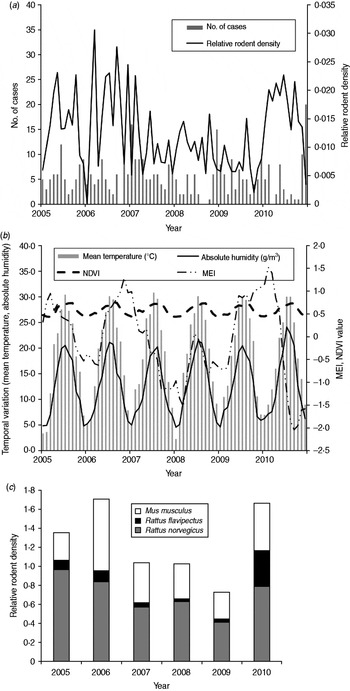
There were 387 HFRS cases in Changsha during the study period, giving an annual average incidence of 1·02/100 000. We observed a peak of HFRS in winter (November–January). Figure 2 shows the temporal variation in environmental variables and the distribution of cases during the study period. A total of 44 206 traps were set and 718 rodents were captured from 2005 to 2010. The rodents, belonging to three species, were captured in residential areas, industrial sites and in rural sites. Rattus norvegicus (55·58%) and Mus musculus (34·95%) were the most predominant species captured, with R. flavipectus representing 9·47% of the total (Fig. 2 c).

Fig. 2. Temporal variation in environmental variables and the number of haemorrhagic fever with renal syndrome (HFRS) cases in Changsha, 2005–2010. (a) The number of HFRS cases and rodent density. (b) Environmental variables and (c) the rodent species composition, 2005–2010. MEI, Multivariate El Niño Southern Oscillation index; NDVI, normalized difference vegetation index.
In the study area, mean temperature, rainfall, absolute humidity, MEI, and NDVI value for rice paddies, orchards, forest land and residential areas were significantly correlated with the monthly notified number of HFRS cases with a lag time of 1–6 months (Table 1).
Table 1. Maximum cross-correlation coefficients of monthly environmental variables and notifications of haemorrhagic fever with renal syndrome: Changsha, China, 2005–2010
MEI, Multivariate El Niño Southern Oscillation index; NDVI, Normalized difference vegetation index.
* P < 0·05, ** P < 0·01.
The Poisson regression model showed that the occurrence of HFRS cases was third-order autoregressive, indicating that the number of notified cases in the current month was related to the numbers of cases occurring in the previous 1, 2 and 3 months (Table 2). Season and long-term trends also made a contribution to the number of disease notifications. After controlling for autocorrelation, seasonality, and long-term trend, relative rodent density at a lag of 2 months and MEI at a lag of 6 months appeared to play significant roles in the transmission of HFRS. The final Poisson regression model suggests that a 1-unit increase in rodent density may be associated with a 33·3% [95% confidence interval (CI) 6·3–67·4] increase in HFRS cases and 1–unit MEI increase may be associated with 66·4% (95% CI 31·5–210·4) increase in HFRS cases, respectively (Table 2). Only final parameter estimates of regression are presented.
Table 2. Parameters estimated by time-series adjusted Poisson regression for haemorrhagic fever with renal syndrome in Changsha*

IRR, Incidence rate ratio; MEI, multivariate El Niño Southern Oscillation index.
* Dummy variables for month were included in the final model.
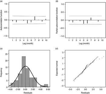
As shown in Figure 3, the estimated/expected number of cases from the final model fits reasonably well for Changsha for the period 2005–2009, as did the 1-year forecast (Fig. 3 a). Figure 3 b compares observed numbers of HFRS cases with predicted numbers from the fitted model; the pseudo-R 2 value for the fitted model was 74·09%. The mean relative prediction error of the model was 22·19% and the standard error of the model prediction was 1·48. In the diagnosis of the residuals of the model, a random distribution was observed with no significant autocorrelation observed (Fig. 4 a, b). Figure 4(c, d) shows the histogram and the normal probability quantile-quantile (Q-Q) plots of the residual data. The Q-Q plot shows the ordered values of data vs. the corresponding quantiles of a standard normal distribution, i.e. a normal distribution with mean zero and standard deviation 1. We used the Kolmogorov–Smirnov statistical test for normality of the distribution (D = 0·148, P < 0·001), and the results indicated that the residuals were normally distributed.

Fig. 3. Observed vs. predicted haemorrhagic fever with renal syndrome cases in Changsha: (a) temporal dynamics and (b) scatterplot.

Fig. 4. (a) Autocorrelation and (b) partial autocorrelation of residuals in Changsha, and the distribution of (c) residuals and (d) Q-Q plot of residuals. The dotted lines in panels (a) and (b) indicate the upper and lower 95% confidence intervals.
DISCUSSION
Our study investigated the association between HFRS infection and rodent density. Findings from this analysis indicate that although temperature, rainfall, absolute humidity, and NDVI are correlated with the number of HFRS cases, the climatic and environmental variables may not have a direct effect on HFRS incidence. It is likely that those variables play a role in HFRS transmission mainly through their effect on the rodent population and that it is the density of the rodent host population that has the greatest effect on HFRS transmission. The time-series adjusted Poisson model suggests that the rodent density [Reference Kallio12] and the MEI are important predictors of the intensity of HFRS transmission in the study area. We also found that the number of new cases in a given month could be related to the number of cases in previous months, which is of great importance in the prediction of epidemics and for disease prevention by health authorities [Reference Zhang19]. For example, our findings will be helpful in providing an early warning system for controlling rodent density and managing the high-risk population prior to potential outbreaks, once a potential increase in HFRS cases has been detected by the HNDSS. Our findings also support the application of time-series adjusted Poisson regression analysis to better understand the complex relationship between environmental factors and rodent-borne infectious diseases [Reference Zhang19].
Climatic factors affect the dynamics and activities of rodents [Reference Vickery and Bider21] and infection by hantaviruses [Reference Yan4, Reference Wei7, Reference Fang22, Reference Bi23]. We used absolute humidity, instead of relative humidity because the former can be of greater biological significance for many organisms [Reference Shaman and Kohn24, Reference Shaman25]. Relative humidity is the ratio of the actual water vapour pressure of air to equilibrium or saturation of vapour pressure of air, whereas absolute humidity is the actual water vapour content of air irrespective of temperature. Absolute humidity and rainfall can affect the transmission of rodent-borne diseases mainly through their effect on the growth of vegetation [Reference Viel26, Reference Ernest, Brown and Parmenter27].
Climate in China, particularly southern China, is affected greatly by ENSO, which is the most important ocean atmosphere phenomenon [Reference Huang and Wu28]. In this study, MEI was used as an indicator of the climate pattern in Changsha, an important variation for characterizing changing patterns of epidemic situations [Reference Bi and Parton29–Reference Hashizume, Terao and Minakawa31]. This result indicated that the epidemic in the study area may be affected by large-scale climatic variation. A possible reason could be that MEI integrates the climatic information and reflects the cycle and nature of the climate in Changsha at a relatively large scale. MEI may be a good indicator for climatic variables, which may affect the intensity of epidemics. Furthermore, it can also reduce the number of variations in the model, thus avoiding problems of collinearity [Reference Chaves and Pascual32].
The lushness of the vegetation may reflect the level of biomass and potentially impact the transmission of HFRS [Reference Boone33]. The NDVI value is closely correlated with the number of HFRS cases in rice paddies (r = 0·271, P < 0·01), orchards (r = 0·346, P < 0·01), the forest (r = 0·269, P < 0·01) and in residential areas (r = 0·334, P < 0·01). In our study although the NDVI is significantly correlated with the number of HFRS cases, it was not significant in the final Poisson model, indicating that vegetation status may affect HFRS incidence indirectly through its effect on the rodent reservoir.
Following the hypothesis that a greater number of reservoir hosts may lead to higher HFRS incidence, due to the higher transmission rate to human [Reference Kallio12], the monthly rodent density was shown to play an important role in HFRS transmission in Changsha (Table 2) with a 2-month lag. Rodent dynamics in turn are influenced by many aspects in the environment. Thus, by monitoring rodent density we can predict potential epidemics ahead of time thus allowing opportunities for controlling the disease, and even preventing the epidemic. The monitoring data show that M. musculus and R. norvegicus are the predominant virus host species, indicating that by killing and controlling these rodent hosts in an area can reduce the disease.
An advantage of this study was the integration of climatic variables with other environmental variables including data on the rodent host reservoir to give a more complete epidemiological analysis of the disease. Some potential time-related confounding variables, e.g. seasonality, lagged effects, long-term trend and autocorrelation, have been controlled in the regression analysis. We also recognize certain limitations of the study, including issues relating to potential underreporting of cases, the use of monthly data, and lack of data on socioeconomic status, which plays an important role in the transmission of infectious disease. Furthermore, as a population-level study, the potential problem of ecological fallacy is always unavoidable in a study of this kind.
In conclusion, the results of this study suggest that antecedent patterns of relative rodent density and MEI were the key determinants of HFRS transmission in Changsha. This method can also be expanded and applied to other new epidemic foci in China and provide a predictive capacity for HFRS epidemics.
ACKNOWLEDGEMENTS
This work was supported by the Key Discipline Construction Project in Hunan province (2008001), the Scientific Research Fund of Hunan Provincial Education Department (11K037), Hunan Provincial Natural Science Foundation of China (11JJ3119), Science and Technology Planning Project of Hunan Province, China (2010SK3007) and the Key Subject Construction Project of Hunan Normal University (geographical information systems). The funders had no role in study design, data collection and analysis, decision to publish, or preparation of the manuscript.
DECLARATION OF INTEREST
None.