


INTRODUCTION
People mastering Rietveld refinement techniques commonly ask the same questions: What do the various Rietveld discrepancy values, i.e., goodness-of-fit, χ 2, and R factors mean? Also, which ones are most important? Finally, what values allow one to distinguish good refinements from poor ones? These questions are also important to people who review Rietveld results, as well as individuals trying to decide if the results in a paper are likely to be trustworthy. These discrepancy values are only one criterion for judging the quality of Rietveld fits; of greater importance is the “chemical reasonableness” of the model. Also, as will be discussed further, graphical analysis of a fit is very valuable.
In this article, I will explain how several of the most important of these discrepancy terms arise, what they mean, and what they measure, as well as slipping in a few of my own opinions—which may not be universally held in the field. But to start with the last question, there is no simple way to distinguish a good fit from one that is just plain wrong based on R factors or other discrepancy values. A large number of Rietveld indices have been proposed, but I have yet to see one that can be used as an absolute measure of refinement quality. The reason for this should be clear by the end of this article, but to get started, let’s define the concepts needed for this discussion. In the following paragraphs, when a term is first defined, it is presented in bold face to make the definition easier to see.
Diffraction data are a set of intensity values measured at a set of specific momentum transfer (Q) values, which are usually expressed as 2θ settings. It should be noted that diffraction measurements can also be made with fixed 2θ while the wavelength varies, for example, in time-of-flight or energy-dispersive diffraction. However, for convenience, I will assume that data are collected as a function of 2θ for this paper. By convention, the intensity values are labeled yO,i, where O indicates these are observed values and i indicates the intensity was measured at 2θ value 2θ i. To perform Rietveld analysis, we must have an uncertainty estimate for yO,i, which I will label σ[yO,i]. In the past, this was called the estimated standard deviation (esd), but crystallographic convention now uses the term standard uncertainty (s.u.) for this (Schwartzenbach et al., Reference Schwartzenbach, Abrahams, Flack, Prince and Wilson1995, Reference Schwartzenbach, Abrahams, Flack, Prince and Wilson1996). The meaning of σ[yO,i] is that if we knew the “true” value for this intensity, which I will label yT, i, say, by measuring it an infinite number of times, then on average yO,i will be ±σ[yO,i] of yT,i. Another way to express this is that <(yO,i−<yO,i>)2>=σ2[yO,i], where < > indicates the expected value. When intensities are measured by directly counting individual photons or neutrons arriving at the detector, e.g., pulse counting, then yO,i=σ2[yO,i]. In cases where intensity values incorporate implicit scaling factors, the s.u. must be computed from the number of counts and then be scaled by the same factor as the intensity. (If yO,i=s I O,i, where I O,i is the actual number of counts, then s 2I O,i=σ2[yO,i].) Examples where this is needed include the use of variable counting times or scaling by a monitor detector or from instruments that report counts per second. Estimation of experimental uncertainties can be quite difficult for detectors that do not directly count quanta, e.g., charge coupled detectors, image plates, or energy-dispersive detectors that automatically correct for detector dead time.
MODEL ASSESSMENT
In Rietveld analysis, we fit a model to the data. If the model is correct then it will predict what the “true” intensity values should be. The intensity values simulated from the model will be labeled as yC,i, where the C indicates they are computed from the model. The Rietveld algorithm optimizes the model function to minimize the weighted sum of squared differences between the observed and computed intensity values, i.e., to minimize Σ iw i(yC,i−yO,i)2 where the weight, labeled as wi, is 1∕σ 2[yO,i]. Other weighting schemes can be used, but when errors are purely statistical in nature, the smallest uncertainties in the fit parameters are obtained where w i=1∕σ 2[yO,i] (Prince, Reference Prince2004; David, Reference David2004). The most straightforward discrepancy index, the weighted profile R-factor (Rwp), follows directly from the square root of the quantity minimized, scaled by the weighted intensities: R wp2=Σ iw i(yC,i−yO,i)2∕Σ iw i(yO,i)2 (Young, Reference Young and Young1993).
As a thought experiment, what happens if we have the ideal model, one which accurately predicts the true value for each yO,i value? In that case, the average value of (yC,i−yO,i)2 will be equal to σ 2[yO,i], and the expected value of wi(yC,i−yO,i)2 is one. The R w p that one would obtain with this ideal model is thus the best possible value that can ever be obtained for that set of data, provided that the σ[yO,i] values are correct. This “best possible R w p” quantity is a very useful concept and is called the expectedRfactor (Rexp). Using N as a label for the number of data points, R exp2=N∕Σ iw i(yO,i)2 (Young, Reference Young and Young1993) (The purist may note that in fact N should be the number of data points less the number of varied parameters, a quantity that statisticians call “degrees of freedom”, but is better considered as the amount of statistical overdetermination; for powder diffraction, the number of data points had better be sufficiently larger than the number of varied parameters such that the subtraction of the latter can be safely ignored.).
A related statistical concept is that of “Chi squared” or χ2. This can be thought about by again considering that the expected value for (yC,i−yO,i)2∕σ 2[yO,i] will be one, when the model is ideal and s.u. values are correct. The χ 2 term is then defined as the average of these values χ 2=(1∕N)Σ i(yC,i−yO,i)2∕σ 2[yO,i] (Young, Reference Young and Young1993). Note that χ 2 can also be determined from the expected and weighted profile R factors χ 2=(R w p∕R exp)2. The single-crystal literature often uses the term goodness of fit (G) which is defined by G 2=χ 2. Goodness of fit is less commonly used in powder diffraction. For reasons unclear to me, one never sees a reference to χ, only χ 2.
During the refinement process, χ 2 starts out large when the model is poor and decreases as the model produces better agreement with the data. Mathematically, least-squares refinement should never cause χ 2 to increase, but in practice small increases do sometimes occur when parameters are correlated. Any large increase is a sign of problems. Other refinement techniques, such as Monte Carlo, intentionally allow χ 2 to increase as a way of avoiding false minima.
It should be noted that χ 2 should never drop below one, or equivalently, the smallest that R w p should ever be is R exp. If a refinement results in χ 2<1, then <(yC,i−yO,i)2> is less than σ 2[yO,i], which means that one of two things is true: (1) The standard uncertainties for the data must be overestimated or (2) so many parameters have been introduced that the model is adjusting to fit noise (which should be unlikely in powder diffraction). When χ 2 is close to one, there is no guarantee that the model is correct—there may be many models that will produce more or less equivalent fits—but the experimental data are not sufficient to produce a more complex and perhaps more correct model. On the other hand, if at the end of a refinement χ 2⪢1, then either: (1) The model is reasonable but the s.u. values are underestimated, (2) the model is incomplete because there are systematic effects (errors) in the data that are not expressed in the model, or (3) the model is wrong. As will be discussed further below, high χ 2 values can occur where data are collected to very high precision; in these cases, minor imperfections in the fit become huge with respect to the experimental uncertainty. However, there are also many cases where χ 2⪢1 indicates results that are completely untrustworthy. There are many fine papers published with refinements where χ 2⪢1, but the reasons why the fit is statistically poor must always be well understood in order to differentiate good results from garbage.
One important test to make when χ 2⪢1 is to note the difference between the χ 2 or R w p value obtained from your model and the value obtained from a Le Bail or Pawley fit, where peak intensities are optimized without the constraint of a structural model (Le Bail et al., Reference Le Bail, Duroy and Fourquet1988; Pawley, Reference Pawley1981). If your crystallographic fit is as good as the Pawley/Le Bail fit, then experimental features in the data (typically peak shape or background) are not being modeled properly, but the crystallographic model can no longer be improved. More detailed analysis is needed to know how these features are affecting the fit of the integrated intensities before knowing if the resulting model can be trusted. If the converse is true and the Le Bail fit provides a good fit but the Rietveld fit does not, then there are systematic crystallographic problems with your model. There are some systems that cannot be described well by conventional models; the result may be very useful even though it is only approximate, but again analysis is needed to understand the suitability of the results.
Having a model where χ 2 is far from unity has a very profound implication with many modern Rietveld programs. The least-squares minimization method used for Rietveld allows the statistical uncertainty in the data to be extrapolated to statistical uncertainty in the optimized values for the model’s adjustable parameters (for example, s.u. values for refined atomic coordinates). These values are derived from the least-squares variance-covariance matrix, but this estimate is accurate only when χ 2≈1 (Prince, Reference Prince2004). Many (but not all) Rietveld programs treat this problem with a Band-Aid, by multiplying the derived s.u. values by G. The reasons for doing this are poorly grounded. If the cause of the large χ 2 is something that has negligible correlation to the parameter in question, for example imperfections in peak shape to atomic coordinates, there is little increase in uncertainty due to the incomplete fit. On the other hand, if there is a significant correlation between an unmodeled effect in the data (a.k.a. a systematic error) with this parameter, the loss of precision may be much larger than the factor of G. As an example of this, consider a fit to a flat-plate sample that is too thin, so that the beam penetrates through the sample. The systematic error due to this penetration will increase with 2θ and thus will skew atomic displacement parameters (“thermal factors”). The induced error in these parameters could be quite severe, and multiplying by G would likely underestimate the uncertainty. In the case where χ 2<1, multiplying the s.u. values by G reduces them, which is a really bad idea.
The last concept I want to introduce, unlike R w p, R exp, and χ 2, has no statistical basis, but is still very valuable as a measure of refinement quality. In single-crystal diffraction, R factors are computed based on the observed and computed structure factors, which can be labeled F O,h k l and F C,h k l, respectively. The F C,h k l values are computed directly from the crystallographic model as an intermediate in Rietveld refinement; but unlike in single-crystal diffraction, F O,h k l values cannot be measured in a powder diffraction experiment due to the superposition of multiple reflections into single peaks. Fortunately, Hugo Rietveld came up with a very nice mechanism for estimating F O,h k l values as part of his method (Rietveld, Reference Rietveld1969). For each point in the diffraction pattern, the intensity is apportioned between the contributing reflections according to the ratio of how the F C,h k l values contribute to the calculated diffraction pattern. This estimates intensity for overlapped reflections according to the ratios of the computed structure factors. The closer the model is to being “correct,” the more valid this process becomes. R factors based on the F C,h k l and F O,h k l values can be computed using the same formulas that are applied for unweighted single-crystal R-factors: R F=(Σ hkl∣F O,hkl∣−∣F C,hkl∣)∕(Σ hkl∣F O,hkl∣) or based on F 2, R F 2=(Σ hklF O,hkl2−F C,hkl2)∕(Σ hklF O,hkl2) (Young, Reference Young and Young1993). The label R Bragg is sometimes used in the Rietveld literature to refer to reflection intensity-based R factors, but this term is ambiguous, as it may refer to R F, R F 2, or even R I [R I=(Σ hklI O,hkl−I C,hkl)∕(Σ hklI O,hkl)].
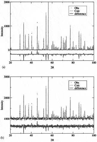
Figure 1. A demonstration of the effect of background on a Rietveld fit. Two simulated fits are shown, where the models have the same discrepancies from the simulated data and where the Bragg intensities and counting times are equivalent. However, in case (a) no background is present, R w p=23% and χ 2=2.54, while in case (b), significant background is present, R w p=3.5% and χ 2=1.31.
DISCUSSION
Now that we have all these R-factors defined, why is it that someone cannot create a rule-of-thumb for at least one of them, where having a value above some threshold is a cause for suspicion, but a value below that threshold indicates a refinement that is generally reliable? One reason is that these indices measure not just how well the structural model fits the diffraction intensities, but also how well we have fit the background and how well the diffraction positions and peak shapes have been fit. If a large percentage of the total intensity in a pattern comes from background, then fitting the background alone can give relatively small χ 2 or R w p values, even without a valid structural model (McCusker et al., Reference McCusker, Von Dreele, Cox, Louër and Scardi1999). Figure 1 shows how significantly these values can be affected by background levels. Another reason a rule-of-thumb test fails is that we can always improve the χ 2 by using other types of lower-quality data. Note that counting longer increases the statistical precision in a diffraction measurement. Indeed, as the total number of counts collected for a diffraction pattern is increased, R exp decreases. Paradoxically, counting longer will usually increase the difference between R exp and R wp and thus make χ 2 worse even though the model obtained by fitting will be improved. This is because, when patterns are measured with very large numbers of counts, even minor “imperfections” (i.e., features that cannot be modeled) in the peak shape or peak positions can make it impossible to obtain small χ 2 or R w p values. The imperfections would be no different with shorter counting times and would produce the same shifts (if any) to the fitted parameters. However, as the number of counts increases, the discrepancies between observed and computed data will become very large compared to the uncertainty in the intensities. Likewise, improved instrumental resolution is a good thing—it often provides more crystallographic observables, so this again allows for more precise (and sometimes more accurate) models. However, as peak profiles become sharper, imperfections again become even more obvious, so again improved data can result in seemingly “worse” discrepancy indices. Thus, when comparing refinements performed with differing instruments or conditions, the higher-quality dataset may provide larger χ 2 or R w p values, even though the model obtained from that data is also of higher quality.
So, if we cannot say a fit with small discrepancy values is of high quality and a fit with large values is of low quality, why bother computing these terms? One reason is these are the only statistically defined parameters that we have; these are the terms to use when comparing different models fit to the same data (deciding exactly how to compare R factors will come in another article). A second reason is that these values should be monitored to see that they drop as we proceed in the refinement, as noted before. When that is not happening, something is going wrong. Finally, when a refinement converges with χ 2 significantly larger than unity, then there are experimental factors that are not being accounted for by the model, i.e., significant systematic errors are present. The source(s) of these errors must be understood and explained to a reader so that it can be decided if the results can be believed.
What about the reflection-based R factor? One purpose for this index is to impress our single-crystal crystallographer colleagues, who may be loath to accept powder diffraction crystallography. They like to see R F in the range of a few percent in single-crystal fits; Rietveld results can frequently be this good or even better. More seriously, the Rietveld peak integration method can be quite accurate even when profiles are irregular. Good agreement between the observed and computed reflection, as demonstrated by obtaining a small value for one of the R Bragg indices, provides a valuable indication that the model is doing a good job of reproducing the crystallographic observations. Conversely, when these values are more than, say, 5% for R F or a bit higher for the other R Bragg indices, then the question must be asked, “Why is the model not fitting better?” Some materials have structures that are more complex than what can be modeled with standard crystallographic approaches; the Rietveld result may be the best that can be done, and may be of great value, but inspection is needed to understand the discrepancies, and this must be discussed as part of any publication. It should be noted that the integration used for the R Bragg indices starts to fail when peaks have very long tails or have significant unmodeled asymmetry, because parts of the peak are not included in the intensity estimate. Also, be aware that R Bragg is biased toward the model, since information from the model is used to apportion intensity between overlapped reflections. In practice, this is not a major problem, but it should be remembered that R Bragg has no statistical validity.
Many, many other R-factor and discrepancy indices have been suggested for use in Rietveld refinements. This would be a very long article indeed, if I reviewed them all. Each has some minor justification. For example, the Durban–Watson statistic measures if the errors between adjacent points are correlated or random. When errors are correlated, peaks are not being fit as well as statistics would predict. However, one knows this from the value of χ 2, as long as experimental standard uncertainties are correct. Background adjusted R factors reduce, but do not eliminate, the contribution of background fitting—except in the cases where background is poorly fit.
In my experience, the most important way to determine the quality of a Rietveld fit is by viewing the observed and calculated patterns graphically and to ensure that the model is chemically plausible. Future articles will discuss these concepts in more detail.
ACKNOWLEDGMENT
Use of the Advanced Photon Source was supported by the U.S. Department of Energy, Office of Science, Office of Basic Energy Sciences, under Contract No. W-31-109-ENG-38.

