


1. Introduction
Variance component models have played an important role in detecting quantitative trait loci (QTL) for the last couple of decades in both animal breeding (Fernando & Grossman, Reference Fernando and Grossman1989; Goddard, Reference Goddard1992; Arendonk et al., Reference Arendonk, Tier and Kinghorn1994; Wang et al., Reference Wang, Fernando, van der Beek, Grossman and van Arendonk1995; George et al., Reference George, Visscher and Haley2000) and human genetics (Goldgar, Reference Goldgar1990; Schork, Reference Schork1993; Fulker & Cardon, Reference Fulker and Cardon1994; Olson, Reference Olson1995; Xu & Atchley, Reference Xu and Atchley1995; Blangero et al., Reference Blangero, Williams and Almasy2001). To construct the variance–covariance matrix of the random QTL effect, identity-by-descent (IBD) probabilities are required. The IBD probabilities describe the correlation structure between individuals with respect to the frequency of their shared (common) alleles. The genetic variance component estimates, and the corresponding likelihoods, are usually calculated using an estimated IBD matrix.
The IBD matrix can be estimated from marker information using either deterministic (Wang et al., Reference Wang, Fernando, van der Beek, Grossman and van Arendonk1995; Pong-Wong et al., Reference Pong-Wong, George, Woolliams and Haley2001; Besnier & Carlborg, Reference Besnier and Carlborg2007) or stochastic algorithms (Thompson & Heath, Reference Thompson and Heath1999; Pérez-Enciso et al., Reference Pérez-Enciso, Varona and Rothschild2000; Mao & Xu, Reference Mao and Xu2005). All these methods actually calculate an average IBD matrix, where each entry is the average frequency of shared alleles, based on partially informative markers. Namely, all the IBD values are known in the statistical models. Instead of using the average IBD matrix, which we refer to as the expectation method (Xu, Reference Xu1996), the uncertainty of the IBD matrix itself may also be included in the likelihood. Such a method accounting for the uncertainty of the IBD matrix is referred to as the distribution method. The likelihood function that the distribution method uses is called the full likelihood function, in contrast to the expectation method that uses an approximated likelihood function.
Comparison of distribution methods with expectation methods has been a thoroughly investigated problem in human genetics, especially for regression models in QTL analysis and genome-wide association studies (GWAS). Using genotype imputation, GWAS can gain power at positions with uncertain genotypes (Marchini & Howie, Reference Marchini and Howie2010) where the expectation method gives good power and accuracy (Kutalik et al., Reference Kutalik, Johnson, Bochud, Mooser, Vollenweider, Waeber, Waterworth, Beckmann and Bergmann2011) by using SNP probabilities as covariates. For QTL analyses based on regression models, the QTL effect is treated as fixed, and several studies have applied the idea of a full likelihood function (Elston & Stewart, Reference Elston and Stewart1971; Morton & Maclean, Reference Morton and Maclean1974; Lander & Botstein, Reference Lander and Botstein1989), which is referred to as the maximum likelihood (ML) method in QTL analysis and has been implemented in, for instance, MAPMAKER-QTL (Lander & Botstein, Reference Lander and Botstein1989). The implementation is based on an Expectation–Maximization (EM) algorithm (Dempster et al., Reference Dempster, Laird and Rubin1977). However, ML estimates based on a regression model can be approximated very well by the simple Haley–Knott (HK) regression (Haley & Knott, Reference Haley and Knott1992), which is the corresponding expectation method using line-origin probabilities as covariates.
In random effect models, the QTL effect is regarded as random, and considering a full likelihood method is still important to avoid losing statistical power (Schork, Reference Schork1993). Replacing the IBD matrix using its expectation can only approximate the ML estimates, and the approximation was shown, by means of simulations, to be non-negligible in the analyses of sib-pairs (Kruglyak & Lander, Reference Kruglyak and Lander1995). To resolve these problems, a weighted likelihood approach has been implemented in the software package Mx (Eaves et al., Reference Eaves, Neale and Maes1996) for the analysis of small human pedigrees where the probability of IBD states are used as weights. However, knowing the distribution of the IBD matrix is crucial for deriving the full likelihood function. In human full-sib studies, the closed form of the joint distribution of the additive IBD matrix and the dominance IBD matrix has been derived, but this is feasible only for pedigrees including small full-sib families (Gessler & Xu, Reference Gessler and Xu1996; Xu, Reference Xu1996). These earlier studies show that the full likelihood function is statistically more powerful and often gives higher likelihood at the QTL.
Three problems were raised from previous studies. First, for animal pedigrees, deriving the distribution of the IBD matrix is infeasible due to the large size. Therefore, approximating the full likelihood function using a Monte Carlo strategy is a reasonable idea but has not been implemented (Xu, Reference Xu1996). Second, full-sib studies in humans calculate IBD probabilities for F 1 individuals. For a crossing design in animals, where e.g. F 2 individuals are studied, deriving the IBD distribution is difficult even for small pedigrees. An application of the distribution method to F 2 individuals has therefore not been investigated before, even though the theory was claimed to be able to extend to different kinds of crosses. Third, when there is inbreeding, for instance, in an F 2 intercross, diagonal elements of the IBD matrix need to be adjusted. After adjusting for inbreeding, the full likelihood theory still holds. If the marker density is low or the markers are partially informative, the difference between the distribution method and the expectation method might be substantial for experimental crosses as well.
The aim of our study is to evaluate the performance of the distribution method in animal intercross designs by assessing the magnitude and direction of bias for the expectation method. We try to account for the above problems and investigate the full likelihood function for animal pedigrees. The rest of this paper is arranged as follows. We first describe the statistical model that our study is based on and introduce the theory about the full likelihood. Two illustrative examples of F 2 pedigrees are simulated, where one is used to show the difference from full-sib studies, and the other is used to show the performance of the distribution method in adjusting the bias of heritability estimates. We compare the distribution method with the expectation method for a real experimental dataset, with simulations based on real genotypes for comparing the power of the two methods. The paper is concluded by discussing possible applications and suggesting future developments.
2. Methods and materials
(i) Models and likelihoods
We consider the variance component QTL model (Fernando & Grossman, Reference Fernando and Grossman1989; Goldgar, Reference Goldgar1990):
where y is the trait response vector for N individuals, β is the fixed effect vector, γ is the multivariate normal-distributed random QTL effect with a zero mean and variance–covariance matrix ![]() and ε is the normal-distributed error term with a zero mean and variance–covariance matrix
and ε is the normal-distributed error term with a zero mean and variance–covariance matrix ![]() . X and Z are the design matrices. σg2 is the genotypic variance and σe2 is the residual variance. Z relates individuals and their inherited allelic substitution effects. Given the IBD matrix Π, the variance–covariance matrix of the phenotype y is
. X and Z are the design matrices. σg2 is the genotypic variance and σe2 is the residual variance. Z relates individuals and their inherited allelic substitution effects. Given the IBD matrix Π, the variance–covariance matrix of the phenotype y is ![]() . The relationship between Π and Z is given by (Rönnegård & Carlborg, Reference Rönnegård and Carlborg2007):
. The relationship between Π and Z is given by (Rönnegård & Carlborg, Reference Rönnegård and Carlborg2007):
To adjust the bias of variance component estimates due to estimating the fixed effects, restricted maximum likelihood (REML) is commonly used instead of ML. If θ=(σg2, σe2)′ is the vector of variance components, the likelihood function is given by

If the alleles cannot be traced unambiguously through the pedigree, e.g. because the markers are not fully informative, the conditional expectation of Π has been used as a known matrix for the estimation of likelihood (3) (expectation method). Regarding Π as random, a joint distribution f(y,Π|θ) is considered for estimating the likelihood (distribution method), i.e. the full likelihood. In this paper, the terms ‘distribution method' and ‘full likelihood method’ are used interchangeably. ℓ is used to denote the logarithm of the corresponding likelihood ![]() .
.
Given the incomplete marker information, there is a probability space in which the IBD matrix Π is distributed. The expectation method uses an approximated likelihood
where the variation of Π is not considered since E[Π] is inserted as a known matrix. Instead of calculating the expected IBD matrix E[Π], the full likelihood function takes the variation of Π into account by considering the joint distribution of θ and Π. Inference of θ should be made from the marginal likelihood of θ integrating out Π. Hence, based on profile likelihood (3), the distribution method uses the marginal likelihood

Thus, the difference between ![]() and
and ![]() is the difference between calculating the function of an expectation and calculating an expectation of the function. Non–linearity of function
is the difference between calculating the function of an expectation and calculating an expectation of the function. Non–linearity of function ![]() with respect to Π affects the difference between
with respect to Π affects the difference between ![]() and
and ![]() .
.
(ii) Computation of the full likelihood
Since the distribution of Π is rather complicated, marginal likelihood (5), involving an expectation with respect to Π, is hardly derivable unless the number of individuals is extremely small. Therefore, we propose a Monte Carlo strategy that approximates likelihood (5) by
where m is the number of imputed IBD matrices drawn based on the marker information. Each impute Πi corresponds to an incidence matrix Zi, and eqn (2) holds, so that ![]() .
. ![]() converges to
converges to ![]() as m→∞, where
as m→∞, where ![]() is the ML estimate of
is the ML estimate of ![]() .
.
The estimate of θ is identical for all the imputes of ![]() , namely, instead of maximizing each imputed likelihood, the entire sum
, namely, instead of maximizing each imputed likelihood, the entire sum ![]() needs to be maximized. The first and second derivatives of
needs to be maximized. The first and second derivatives of ![]() with respect to θ have closed solutions (Harville, Reference Harville1977). Let
with respect to θ have closed solutions (Harville, Reference Harville1977). Let ![]() and
and ![]() . ℓ is the target log-likelihood to maximize. Using the derivatives
. ℓ is the target log-likelihood to maximize. Using the derivatives ![]() and
and ![]() , a Newton–Raphson-based EM algorithm can be used to estimate θ.
, a Newton–Raphson-based EM algorithm can be used to estimate θ.
Algorithm. Given a set of imputed IBD matrices (or corresponding incidence matrices), estimation of variance components θ using the full likelihood function can be made via the following steps:
(i) Find an initial estimate
 .
.(ii) Loop on k until convergence.
(7)where δ is a step size constant and(8)(9)In eqns (8) and (9), the weights are defined as(10)(iii) Take the converged estimate
as the final variance component estimates.
This algorithm is based on Newton–Raphson iterations but is an EM algorithm since the weights in gradient and hessian need to be updated using the current variance component estimates. There are two advantages with this implementation. First, imputing incidence matrices (Zi) is much easier than creating the IBD matrices (Πi) that is not required in the proposed algorithm. Second, for large pedigrees with a few founders, when the marker is partially informative, the rank of ![]() is much greater than the rank of Zi. A low rank of Zi increases the computational efficiency for maximizing the likelihood function (Rönnegård et al., Reference Rönnegård, Mischenko, Holmgren and Carlborg2007).
is much greater than the rank of Zi. A low rank of Zi increases the computational efficiency for maximizing the likelihood function (Rönnegård et al., Reference Rönnegård, Mischenko, Holmgren and Carlborg2007).
(iii) Simple illustrative examples
Two pedigrees were simulated for showing different properties of the method. Pedigree I was simulated for showing that the non-negligible bias from the expectation method could be adjusted by the distribution method. Pedigree II was simulated for showing that the proven relationship between the likelihood estimate from the expectation method and that from the distribution method for full-sib families is not true for F 2 intercrosses.
(a) Pedigree I
In an F 2 intercross (Fig. 1 a), a single pair of grandparents were mated to produce one male and two female F 1 progeny. They were thereafter mated to obtain five F 2 offspring. At a putative QTL, genotypes were simulated for each individual, and there are four alleles (A, B, C and D) throughout the pedigree. The phenotypic value for individual i was simulated by
where μ=50, ![]() , and γi1 and γi2 correspond to the paternal and maternal allele substitution effects. Five sets of allele substitution effects were simulated according to five different σg2 values. For instance, given the sample variance of σg2=15, the allelic effects can be assigned as γA=3, γB=6, γC=9 and γD=12, which give a consistent estimate for the genetic variance, and the simulated phenotypic values were 64·87, 56·21, 61·28, 69·20 and 62·08 for individuals 6–10, respectively, for this particular set of allelic effects. In Fig. 1 a, the kinship information is known but the genotypes are not observed. The (narrow sense) heritability (Lynch & Walsh, Reference Lynch and Walsh1997) of the studied trait is defined as the intra-class correlation by
, and γi1 and γi2 correspond to the paternal and maternal allele substitution effects. Five sets of allele substitution effects were simulated according to five different σg2 values. For instance, given the sample variance of σg2=15, the allelic effects can be assigned as γA=3, γB=6, γC=9 and γD=12, which give a consistent estimate for the genetic variance, and the simulated phenotypic values were 64·87, 56·21, 61·28, 69·20 and 62·08 for individuals 6–10, respectively, for this particular set of allelic effects. In Fig. 1 a, the kinship information is known but the genotypes are not observed. The (narrow sense) heritability (Lynch & Walsh, Reference Lynch and Walsh1997) of the studied trait is defined as the intra-class correlation by

which measures how large proportion of the trait variation is determined by inheritance. We used both the expectation and the distribution method to estimate h 2 using the five animals in the F 2 generation. Note that equivalently, this example compares the variance component estimates using the two methods given an uninformative marker (no marker information) in QTL analyses.
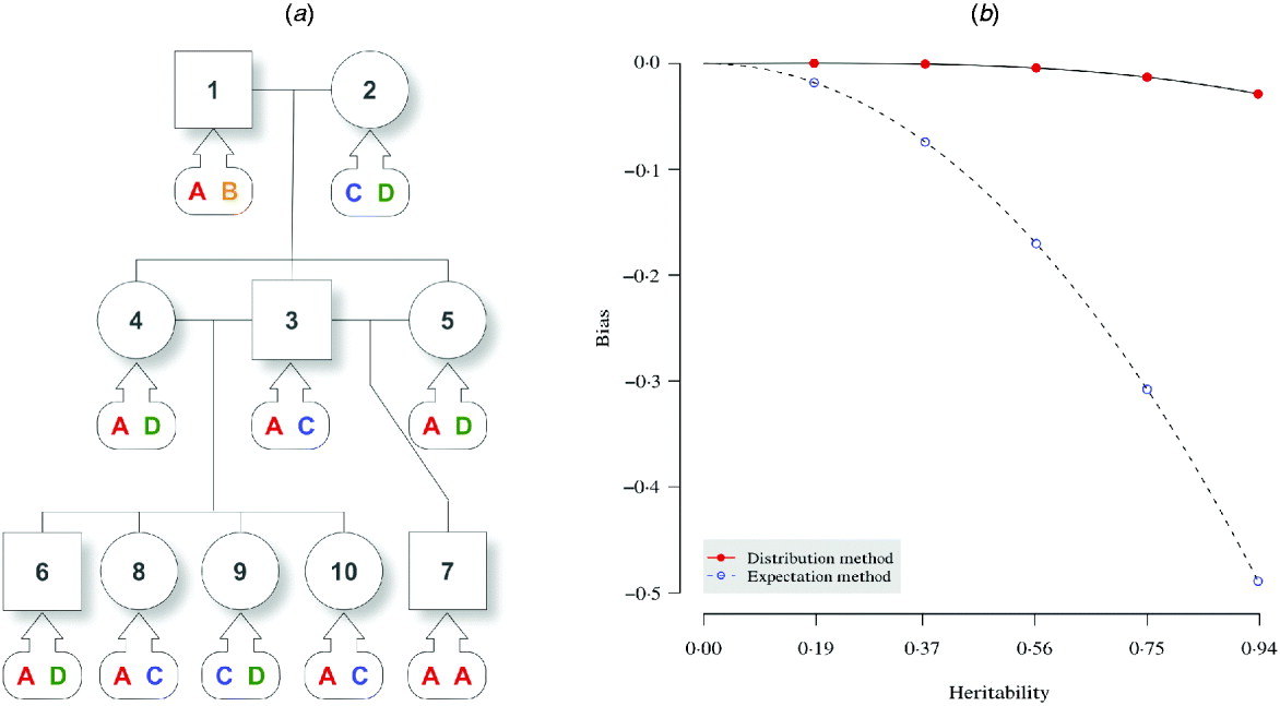
Fig. 1. Pedigree I – a simulated F 2 intercross with 10 individuals including two founders. (a) A three-generation intercross with five offspring, three parents and two grandparents. Squares and circles denote male and female animals, respectively, with indices inside. Bubbles with arrows pointing to each animal indicate the true genotypes that are not observed. (b) For the distribution method and the expectation method, asymptotic trend of bias in estimating the narrow sense heritability is displayed with respect to the heritability of the trait.
(b) Pedigree II
One male was mated to three females to produce six F 1 individuals, and the F 1s were mated to obtain 10 F 2 offspring (Fig. 2). At a putative QTL, allele substitution effects for the eight alleles of the founders were simulated from a normal distribution with a zero mean and a standard deviation of 3, and they were inherited through the pedigree (Table 1). The phenotypes were calculated by summing the allele substitution effects, an overall mean of 200 and an error term drawn from ![]() . Assuming a complete link to the QTL, two sets of marker genotypes were simulated (Markers I and II). We computed the log-likelihood function using both the expectation and the distribution method.
. Assuming a complete link to the QTL, two sets of marker genotypes were simulated (Markers I and II). We computed the log-likelihood function using both the expectation and the distribution method.
Fig. 2. Pedigree II – a simulated F 2 intercross with 18 individuals including four founders. Squares and circles denote male and female animals, respectively, with indices inside. Each dashed curve connects the same individual for the purpose of clear display.
Table 1. The tabular form of pedigree II. Two markers that have a complete link to the QTL were simulated. ℓD and ℓE are log-likelihood from the distribution method and the expectation method, respectively. Given marker I, ℓ D>ℓ E, while given marker II, ℓ D<ℓ E.
(iv) Analyses of experimental data
(a) Simulation using real genotypes
An F 2 cross was bred from two European wild boars mated to eight large white sows (Andersson et al., Reference Andersson, Haley, Ellegren, Knott, Johansson, Andersson, Edfors-Lilja, Fredholm, Hansson, Håkansson and Lundström1994). Four F 1 boars were mated to 22 F 1 sows to produce 191 recorded F 2 offspring in 26 families. The genetic information on chromosome 6 came from 22 genotyped micro-satellite markers at 0·0, 8·6, 36·6, 49·7, 50·5, 62·9, 79·2, 80·4, 83·7, 84·1, 84·8, 90·6, 95·4, 100·7, 101·9, 115·9, 116·7, 119·0, 120·2, 124·0, 127·0 and 170·9 cM. In order to investigate the power of the distribution method and the expectation method for this real dataset, we simulated a QTL at 25 cM harboured by the two flanking markers at 8·6 and 36·6 cM. This simulated QTL position has low marker information since it is in the middle of the longinterval between two markers with low information content. IBD probabilities at the QTL were calculated taking into account all the marker information across the chromosome. We simulated the phenotype under three different scenarios for the heritability, 90%, 10% and 0%. For each scenario, 1000 replicates were simulated, where for each replicate, we calculated the LRT statistics both for the expectation and the distribution methods.
(b) Analysis of a real phenotype
A meat quality trait (reflectance value, EEL) recorded in the pig cross is strongly affected by the halothane gene located on chromosome 6 at position 80·4 cM. One of the founder boars was heterozygote (Hal N/Hal n) for this gene while all the other founders were homozygotes (Hal N/Hal N) for the wild-type allele. In our analyses, we include sex, litter and slaughter weight as fixed effects (Knott et al., Reference Knott, Marklund, Haley, Andersson, Davies, Ellegren, Fredholm, Hansson, Hoyheim, Lundström, Moller and Andersson1998). The causal mutation underlying this QTL had previously been evidenced by Lundström et al. (Reference Lundström, Karlsson, Håkansson, Hansson, Johansson, Andersson and Andersson1995), and the dataset is here used to illustrate the properties of both the expectation and the distribution method. The statistic used for QTL scan was the likelihood-ratio test (LRT) statistic that which is equivalentto the maximized likelihood function value but always non-negative. A permutation test was performed to obtain a significance threshold.
To understand the informativeness of each marker, the polymorphism information content (PIC) was used and determined using the following equation:

where p i is the frequency of the ith allele and t is the number of alleles (Botstein et al., Reference Botstein, White, Skolnick and Davis1980).
3. Results and discussion
(i) Simple illustrative examples
(a) Pedigree I
The conventional expectation method estimates h 2 using likelihood (4), where the variance–covariance matrix of the genetic random effect is the relationship matrix in this example, since it is assumed that no marker information is known. Hence, for the F 2 individuals the expected IBD matrix is

The simulated true value of h 2 is given by s γ2/(s γ2+σe2), where γ=(γA, γB, γC, γD)′, i.e. the vector of allelic effects, and s represents the standard deviation.
The aim here was to estimate the heritability h 2 by estimating the variance components σg2 and σe2. For the simulation with σg2=15, the simulated true h 2 is 0·9375. The estimate by the distribution method converged to 0·9087 using 10 000 Monte Carlo imputes, and the bias was therefore, −0·0288 (Table 2). The expectation method using the expected IBD matrix (14) gave an estimate of 0·4485 and a bias of −0·4890. The comparison of all the five sets of simulated allelic effects shows an asymptotic trend of the bias by both methods, with respect to heritability (Fig. 1 b). The results show that the difference between the two methods increases with the heritability, and this is consistent with the comparison done in full-sib families (Xu, Reference Xu1996). From this example, the distribution method tends to be robust in variance component estimation and more reliable than the expectation method. For large sample or low heritability, the difference between the two methods will become small; however, the distribution method still gains power, which we show in the analyses of experimental data.
Table 2. Heritability estimates for pedigree I. Using the distribution method, variance components were estimated with different number of Monte Carlo imputes. Compared to the simulated true value, the heritability estimated by the distribution method had much less bias than that estimated by the expectation method.
* Narrow sense heritability, defined as σg2/(σg2+σe2).
(b) Pedigree II
The purpose of this simulated example was to show that the relationship ℓD>ℓE that has been proved for full-sib families (Xu, Reference Gessler and Xu1996) does not always hold, not to compare the two methods. We show here that this inequality does not hold for F 2 intercross designs. Based on the information of marker I, the maximized log-likelihood value of the distribution method was greater than that of the expectation method. However, the inequality was reversed for marker II (Table 1).
It has been claimed that the distribution method is more powerful in QTL detection due to larger likelihood estimates. It is not always true that larger likelihood estimates will lead to more powerful QTL detection, because the likelihood estimates for non-QTL positions might also be inflated. Thus, a QTL detection method gains power when the interval harbouring the QTL produces a relatively larger likelihood than those intervals not harbouring any QTL. As shown above, the inequality ℓD>ℓE does not necessarily hold in F 2 intercrosses, but this does not mean that the expectation method is potentially more powerful in QTL detection. In order to assess this question for the two methods, a larger simulation and a full genome scan need to be performed (see the next subsection).
(ii) Analyses of experimental data
(a) Simulation using real genotypes
For each of the 1000 replicates, we compared the log-likelihood values (equivalent to LRT statistics) from the two methods, namely, the power of detecting the simulated QTL harboured by two flanking partially informative markers (Fig. 3). Since the sample size in this simulation was much bigger than the previous two illustrative examples, the approximation of the expectation method was better so that the result from it is closer to the distribution method. However, for a heritable trait, the distribution method is more powerful than the expectation method (Fig. 3 a, b). When the heritability is low (10%), the distribution method still gains power (Fig. 3 b). When the heritability is 0% (no QTL effect, non-heritable), the distribution method produces significantly less (P-value =2·3×10−14 from a Wilcoxon test) false positives than the expectation method (Fig. 3 c). This suggests that the distribution method has a tendency to improve location accuracy in a variance component QTL scan, which is also found in the analysis of a real phenotype (see below).
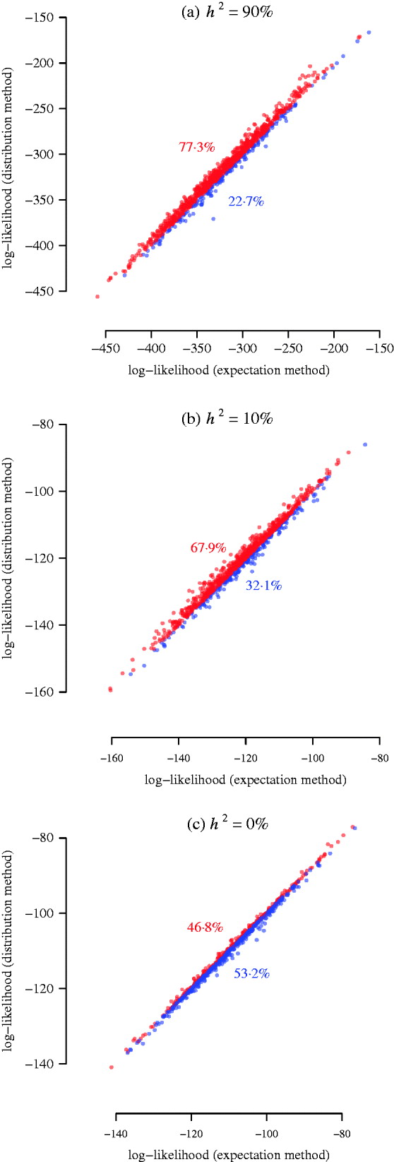
Fig. 3. Simulation results for power of interval mapping. A QTL was simulated at 25 cM of pig chromosome 6. The two markers flanking the interval harbouring the QTL are located at 8·6 cM and 36·6 cM. The real experimental genotypes for 191 F 2 individuals were used to simulate phenotypes, assuming a narrow sense heritability of 0·9, 0·1, and 0. 1000 simulations were used for comparing the log-likelihood from the expectation and the distribution methods. The points above/below the diagonal are in red/blue, indicating that the distribution method has larger power than the expectation method (a, b), or that the distribution method has lower false positive rate than the expectation method (c). The numbers in colour show the corresponding percentages of the sets of points.
(b) Analysis of a real phenotype
A variance-component–based QTL scan was performed on chromosome 6 for the European wild boar×large white intercross (Fig. 4). Both the expectation and the distribution method detected a significant signal but with different intervals harbouring the QTL. The conventional expectation method provided an interval longer than 20 cM, but the scan using the full likelihood function refined the peak and shortened the interval down to around 10 cM.
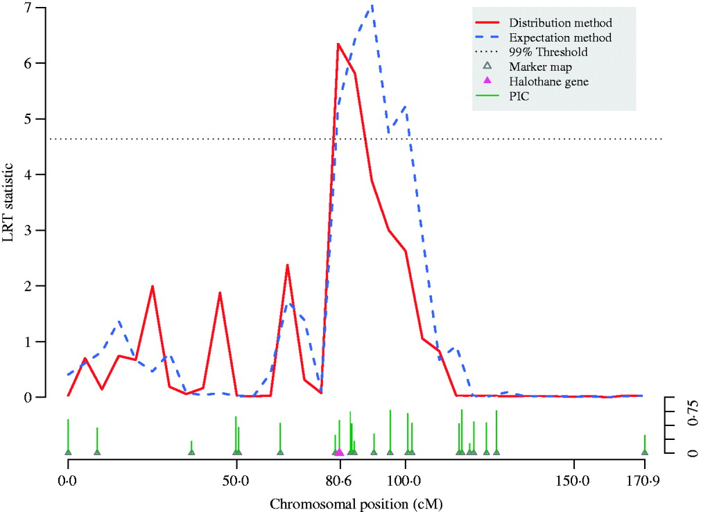
Fig. 4. QTL scan using LRT statistic along pig chromosome 6. The meat quality trait (reflectance value, EEL) is strongly affected by the halothane gene located at 80·4 cM on the chromosome. By adjusting bias of likelihood estimates, thedistribution method refined the peak of the traditional variance component QTL scan using the expectation method and thereby shortened the confidence interval for the QTL. Information for each micro-satellite marker is shown as their PIC.
As shown in our first illustrative example above, the expectation method has a tendency of underestimating the genetic variance at a QTL. Furthermore, it might also overestimate the genetic variance at tested loci with no QTL that are linked to the QTL. Based on our simulations, analyses and the results from previous studies (Gessler & Xu, Reference Gessler and Xu1996), we conclude that the expectation method is a compromising approximation, which loses power of localizing QTL compared with the full likelihood method.
(iii) Further extensions and developments
Epistasis has been emphasized to be common and important in genetic control of complex traits (Carlborg & Haley, Reference Carlborg and Haley2004). A potential extension for our implemented algorithm is to extend it for detecting epistasis, and the idea is straightforward. Consider the variance component model including epistatic effects as
where vA and vB are the main random QTL effects of loci A and B, with ![]() , and vAB is the random interaction effect, where
, and vAB is the random interaction effect, where ![]() denotes covariance. The IBD matrix ΠAB for the epistatic effects in the variance structure of model (19),
denotes covariance. The IBD matrix ΠAB for the epistatic effects in the variance structure of model (19), ![]() , can be calculated as the Hadamard product of the two IBD matrices at loci A and B (Stern et al., Reference Stern, Duggirala, Mitchell, Reinhart, Sivakumar, Shipman, Uresandi, Benavides, Blangero and O'Connell1996), i.e.
, can be calculated as the Hadamard product of the two IBD matrices at loci A and B (Stern et al., Reference Stern, Duggirala, Mitchell, Reinhart, Sivakumar, Shipman, Uresandi, Benavides, Blangero and O'Connell1996), i.e. ![]() . If the expectation method is applied, ΠAB is estimated as
. If the expectation method is applied, ΠAB is estimated as ![]() , which is not always a good approximation if the two loci are linked (Rönnegård et al., Reference Rönnegård, Pong-Wong and Carlborg2008). Using our proposed algorithm, after getting a number of Monte Carlo imputes for the IBD matrices atloci A and B, the full likelihood can be approached by
, which is not always a good approximation if the two loci are linked (Rönnegård et al., Reference Rönnegård, Pong-Wong and Carlborg2008). Using our proposed algorithm, after getting a number of Monte Carlo imputes for the IBD matrices atloci A and B, the full likelihood can be approached by
Substituting the sum into eqn (6), the same EM algorithm can be applied.
In the sample space of Π, there exists a model-based ‘best’ IBD matrix based on the maximum full likelihood. This implies, after profiling out (estimating and inserting back into likelihood) the fixed effects, as in eqn (3), that the best IBD matrix and its corresponding estimate of ![]() maximize the joint likelihood
maximize the joint likelihood ![]() (θ, Π|y). By maximizing the joint likelihood with respect to θ and Π simultaneously, it is possible to infer the best IBD matrix and thereby the best variance component estimates. Nevertheless, our algorithm is not implemented for maximizing the joint likelihood but the marginal. More advanced methods, e.g. those used in phylogenetic tree estimation, using the optimality criterion of ML, often under a Bayesian framework, might be utilized to estimate variance components and the incidence matrix jointly (Felsenstein, Reference Felsenstein2004). Identifying the optimal IBD matrix is NP-hardFootnote 1 using these methods, and so heuristic search and optimization methods most likely need to be used to identify a reasonably good incidence matrix that fits the data. In genetic applications, using Bayesian methods, Gibbs sampling can be used to estimate the incidence matrix; however, it is not guaranteed that the chain is irreducible in large complex problems, and even if the chain is irreducible, mixing can be quite slow (Sorensen & Gianola, Reference Sorensen and Gianola2002). Bayesian computation can be introduced when it is possible and reasonable to joint-estimate the model, otherwise, inference should focus on the variance components. Hence, we suggest that our suggested full likelihood method should be used rather than Bayesian joint estimation of variance components and the true IBD matrices at each putative QTL position.
(θ, Π|y). By maximizing the joint likelihood with respect to θ and Π simultaneously, it is possible to infer the best IBD matrix and thereby the best variance component estimates. Nevertheless, our algorithm is not implemented for maximizing the joint likelihood but the marginal. More advanced methods, e.g. those used in phylogenetic tree estimation, using the optimality criterion of ML, often under a Bayesian framework, might be utilized to estimate variance components and the incidence matrix jointly (Felsenstein, Reference Felsenstein2004). Identifying the optimal IBD matrix is NP-hardFootnote 1 using these methods, and so heuristic search and optimization methods most likely need to be used to identify a reasonably good incidence matrix that fits the data. In genetic applications, using Bayesian methods, Gibbs sampling can be used to estimate the incidence matrix; however, it is not guaranteed that the chain is irreducible in large complex problems, and even if the chain is irreducible, mixing can be quite slow (Sorensen & Gianola, Reference Sorensen and Gianola2002). Bayesian computation can be introduced when it is possible and reasonable to joint-estimate the model, otherwise, inference should focus on the variance components. Hence, we suggest that our suggested full likelihood method should be used rather than Bayesian joint estimation of variance components and the true IBD matrices at each putative QTL position.
In principle, the distribution method derived in this paper can be extended to any general pedigree or population, as long as the genotype probabilities can be calculated. Namely, the algorithm itself has no assumption on the design. Using the genotype probabilities calculated from half-sib designs, backcrosses, advanced intercross lines, or even imputed SNP data from population–based studies, the distribution method can be applied in all situations. The key motivation for using the distribution method is to deal with genotype uncertainty. In experimental crosses, the Monte Carlo step samples IBD matrices, whereas for imputed data in GWAS, we might sample IBS (identity-by-state) matrices. For GWAS using real–typed SNPs, there is no need to apply a full likelihood method as there is no difference between the distribution method and the expectation method when the real genotypes are observed.
4. Conclusion
We have evaluated a full likelihood approach based on variance component QTL models for intercross populations. By means of simulation, we have shown that the full likelihood method is able to correct bias of the traditional variance component method using expected IBD matrices. Also, we used simulations to show that the previously reported relationship between the likelihoods of the distribution and expectation methods does not always hold in general pedigrees. The full likelihood method was compared with the expectation method in experimental cross data, and the former was found to be able to improve the precision of QTL detection. The algorithm described in this paper has been implemented in a package written in R (R Development Core Team, 2010) and is available on request.
Xia Shen is funded by a Future Research Leaders grant from Swedish Foundation for Strategic Research (SSF) to Örjan Carlborg. Lars Rönnegård is funded by the Swedish Research Council for Environment, Agricultural Sciences and Spatial Planning (FORMAS). We thank Carl Nettelblad for providing his programme particularly for our implementation. Leif Andersson is acknowledged for sharing the experimental pig data.


