


Introduction
When it comes to mineral synthesis, there is a lot we can learn from nature. Although we can synthesize a range of materials in the laboratory, the experimental conditions are often constrained to particular ranges of temperature, pH, etc. Biological systems, on the other hand, seem to be able to produce individual minerals and complex composite mineral structures under a variety of conditions, many of which are far from those applied to create their synthetic counterparts [Reference Weiner1]. Understanding how nature does this could provide a means to produce novel biomimetic materials with potential applications in a diverse range of fields from medicine to materials engineering [Reference Bar-Cohen2].
The teeth of chitons (marine molluscs, see Figure 1a) represent an excellent example of a composite biomineralized structure, comprising variable layers of iron oxide, iron oxyhydroxide, and apatite (calcium phosphate). The Biomineralization Group at The University of Western Australia has had an interest in this system for several years [Reference Shaw, Clode, Brooker, Stockdale, Saunders and Macey3, Reference Shaw, Macey, Clode, Brooker, Webb, Stockdale and Binks4, Reference Saunders, Kong, Shaw, Macey and Clode5, Reference Shaw, Clode, Brooker, Stockdale, Saunders and Macey6]. The teeth, which are used to scrape algae growing on and within rocks, are mounted on a long ribbon-like organ termed the radula, with immature, unmineralized teeth at the posterior end and hardened iron-mineralized teeth at the anterior end (Figure 1b). At any one time, up to 80 individual tooth rows can be observed, with each row becoming progressively mineralized as it moves forward in a conveyor belt-like manner.
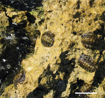
Figure 1a: Chitons (marine molluscs) on rocks at Woodman Point in Perth, Western Australia. Scale bar = 5 cm.
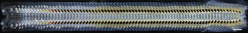
Figure 1b: Light micrograph of the radula feeding organ removed from the chiton. The teeth at the posterior end of the radula (left) start as an unmineralized organic scaffold (clear teeth), and as they move towards the anterior end become progressively mineralized with iron (black teeth). Scale bar = 1 mm.
The early stages of the biomineralization process can be well characterized by a variety of microscopy and micro-analytical techniques [Reference Shaw, Clode, Brooker, Stockdale, Saunders and Macey3]. For example, TEM samples can be prepared by conventional tissue processing techniques allowing thin sections to be readily obtained [Reference Shaw, Macey, Clode, Brooker, Webb, Stockdale and Binks4]. The hard, fully mineralized teeth are a more difficult proposition, however, as standard biological sample preparation methods for TEM can no longer be applied. Studies of mineralized teeth have therefore been limited to techniques such as x-ray diffraction, Raman spectroscopy and scanning electron microscopy (SEM), where the preparation of suitable samples is relatively routine. Although these techniques have provided glimpses of the underlying microstructure (Figure 2) [Reference Shaw, Clode, Brooker, Stockdale, Saunders and Macey3, Reference Lee, Webb, Macey, van Bronswijk, Savarese and de Witt7], they have lacked the spatial resolution to provide vital information on the fine-scale structure and chemistry, particularly at interfaces between the various mineral phases.
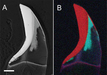
Figure 2: SEM image of a single chiton tooth in longitudinal section during the process of apatite mineral-ization of the core. (A) The back-scatter image shows mass variation in the tooth with the core region partially filled with apatite. (B) Composite element map obtained by energy-dispersive x-ray microanalysis with iron (red), phosphorous (green), and calcium (blue). Scale bar = 50 μm.
We have obtained detailed information about the micro-structure and composition of these mineralized structures by using focused ion beam (FIB) processing to produce precise cross sections from fully mineralized teeth. Several sections were prepared from different regions of a single tooth and at different orientations to the mineral phases. This has enabled us to apply a range of TEM techniques, including conventional imaging, selected area diffraction (SAD), energy-filtered TEM (EFTEM), electron energy-loss spectroscopy (EELS), and high-angle annular dark field (HAADF) STEM imaging to gain new insights into these biomaterials. Using this combination of TEM imaging and analytical techniques, our goals included: (a) to investigate if the mineral phases identified in earlier bulk analyses are the only ones present or if the ability to study these materials at higher spatial resolution would reveal additional phases, (b) to analyze the grain size/morphology of the various mineral phases, (c) to characterize the structural and compositional properties of the interfaces between the mineral phases.
FIB Processing
Although the application of FIB methods in general biological research is constrained by the rapid damage produced in soft tissue, this method is ideally suited to our biomineral studies as the hard, composite tooth structure is comparable to the typical materials science samples where FIB processing is widely utilized.
The first phase of specimen preparation is similar to that used for SEM analysis. Radulae were excised from freshly collected specimens and cleaned using a fine water jet to remove the epithelial tissue surrounding the teeth. They were then fixed and dehydrated prior to resin embedding [Reference Shaw, Clode, Brooker, Stockdale, Saunders and Macey3, Reference Shaw, Macey, Clode, Brooker, Webb, Stockdale and Binks4]. Sample blocks were trimmed such that the face of the block revealed a longitudinal section along the radula. Once orientated, samples were placed in aluminum ring molds and re-embedded in Procure-Araldite. Sections through the major lateral teeth were obtained by polishing these samples with a graded series of Struers silicon carbide papers up to 4000 grit. The final polishing step was performed with 1 μm diamond paste before coating with 50 nm of gold.
A dual-beam FIB system (FEI Nova NanoLab 200) at the University of New South Wales was used to prepare the TEM sections from fully mineralized major lateral teeth. In order to investigate the individual mineral layers and the interfaces between them, sections were acquired from the iron oxide—iron oxyhydroxide interface, the iron oxyhydroxide—calcium apatite interface and across the three mineral layers. Sections involving the calcium apatite layer were more difficult to prepare, as this material is much softer than the iron layers resulting in preferential thinning of, and increased damage to, the apatite. However, with care, high-quality sections could be prepared across the full composite structure.
The electron beam imaging mode was used to locate regions of interest (ROIs) in the polished SEM sample and to monitor the progress of the TEM section preparation during FIB processing. A strip of Pt (approximately 20μm × 2μm × 1μm) deposited in the FIB with a built-in gas injection source system was used to protect the top surface of the ROI. Each TEM section was prepared by a series of steps involving different beam energies and currents resulting in a high-quality section with minimal surface damage and redeposition of material.
First, material on both sides of the ROI was removed with an energetic Ga ion beam operating at 30 kV at a beam current of 5 nA. A wedge-shaped slab of sample, approximately 18μm × 3μm × 5μm in size, remained between the FIB troughs (Figure 3a). Next, the surface damage layers created by the ion beam on both sides of the slab by this initial high-energy milling were removed by a sequence of milling steps involving the use of smaller beam currents, for example 1 nA and 0.3 nA, during a cleaning and thinning process. The resulting section, approximately 15μm × 3μm × 0.8 m, was cut free at one end and along the bottom with a 0.3 nA ion beam at a tilt angle of 45 degrees, leaving the section attached at one end only.
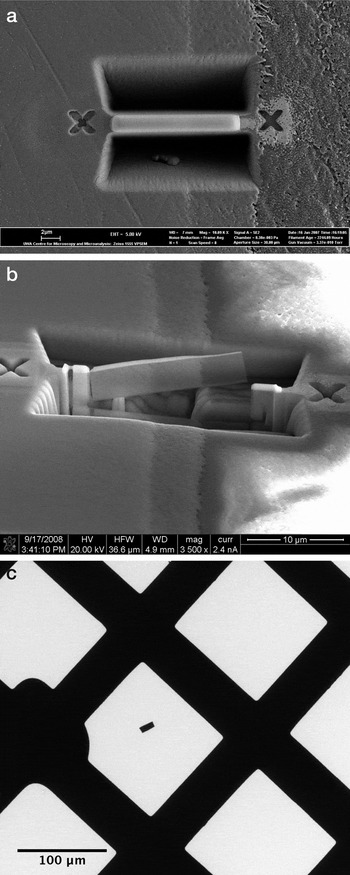
Figure 3: Images of the FIB processing steps with (a) the initial troughs cut on either side of the section, (b) the thin, final lamella having been cut from the surrounding material, and (c) the extracted FIB section sitting on the C-coated TEM grid.
In a final thinning and cleaning step, the blade-shaped section with the Pt protection layer on the top was thinned to less than 100 nm by applying the ion beam alternately to both sides of the sample, with an ion beam current of 0.1 nA. Redeposited dust generated during the earlier processing steps was then carefully cleaned from the surface of the final membrane by line scanning of the ion beam. To extract the prepared section, the remaining fixed end of the membrane was cut with the ion beam (Figure 3b), freeing the section, and an ex-situ micromanipulator system (Kleindiek) was used to remove the section under an optical microscope and mount it on a formvar filmed, C-coated Cu grid for TEM analysis (Figure 3c).
Microstructural and Compositional Characterization
The TEM sections were imaged at 200 kV using a JEOL 2100 LaB6 microscope equipped with a Gatan Orius digital camera, Gatan Tridiem energy-filter, and JEOL STEM detectors. The various layers in the composite mineral structure were clearly visible in the FIB sections (Figure 4). The organic scaffold on which the precursor minerals form was also observed. Previous studies of the mineralized teeth by SEM and Raman spectroscopy indicated that the minerals present were magnetite, lepidocrocite (γ-FeOOH) and calcium apatite [Reference Lee, Webb, Macey, van Bronswijk, Savarese and de Witt7]. Our TEM analysis, however, showed that the situation was more complicated once the fine scale detail could be resolved.
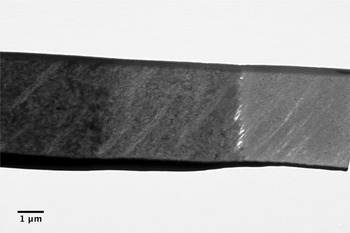
Figure 4: Bright field image of a FIB processed section of a chiton tooth showing the magnetite region (left), goethite/lepidocrocite region (right), and calcium apatite region (right). The dark layer at the bottom of the section is the Pt protective layer deposited during the FIB processing.
Selected area diffraction was used to confirm the presence and distribution of the various mineral phases (Figure 5). While the previously identified magnetite and apatite layers were again observed, the central iron oxyhydroxide layer was found to contain two different phases. Rather than the pure lepidocrocite phase reported by Lee et al. [Reference Lee, Webb, Macey, van Bronswijk, Savarese and de Witt7], the TEM analysis showed that the layer was predominantly made of goethite (α-FeOOH), with lepidocrocite being constrained to a layer a few hundred nanometers thick at the iron oxyhydroxide-apatite interface [Reference Saunders, Kong, Shaw, Macey and Clode5]. In addition, a previously unreported amorphous calcium apatite layer was discovered at the boundary between the apatite and the lepidocrocite [Reference Saunders, Kong, Shaw, Macey and Clode5].
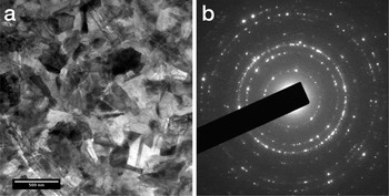
Figure 5: Bright field image and selected area diffraction pattern from the magnetite layer confirming the polycrystalline nature of this region. Diffraction patterns from the other layers confirm the presence of goethite, lepidocrocite, and apatite.
The microstructure was further investigated by HAADF STEM imaging (Figure 6). The mass contrast in the HAADF image shows the delineation between the phases. As the two iron oxyhydroxide phases are almost identical in mass, we are not able to differentiate the border between these phases from the HAADF image. It is only through the use of selected area diffraction that the arrangement of these two phases can be determined.
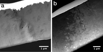
Figure 6: HAADF STEM images of (a) the iron oxyhydroxide-apatite interface with goethite (bright, left), needles of lepidocrocite (bright, middle) extending into the apatite (right, dark) and (b) the iron oxyhydroxide-magnetite interface with goethite (dark, left) and large, angular crystals of magnetite (bright, right). The protective Pt strip from the FIB processing appears bright at the top of both images.
At the elemental level (Figure 7a–d), EFTEM allows us to map compositional changes across the various interfaces and image the underlying organic matrix within the mineralized structure. The compositional data is consistent with the structural and mass-dependent data obtained using the other imaging and diffraction techniques.
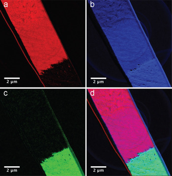
Figure 7: EFTEM element maps showing magnetite (top left), iron oxyhydroxide (middle layer), and apatite (bottom right), with protective platinum and gold layers on surface (left edge); (a) Iron EFTEM elemental map obtained with Fe-L2,3 edge; (b) Oxygen EFTEM elemental map obtained with O-K edge; (c) Calcium EFTEM elemental map obtained with Ca-L2,3 edge; (d) Montage of Fe, O, and Ca maps.
The FIB section thickness (~100 nm) is well suited to analysis by this combination of TEM imaging, diffraction, and elemental maIB processing to prepare high-quality TEM samples across specific features of interest within the teeth and at controlled orientations across the various phases has provided significant new insights into these complex, composite biomineralized structures. The information gained extends our knowledge beyond that obtained by lower-resolution methods. Further studies of this kind are now planned to investigate the evolution of the biomineral microstructure in different teeth along the radula and at other locations and orientations within individual teeth.
Acknowledgment
The authors acknowledge the facilities, scientific, and technical assistance of the Australian Microscopy & Microanalysis Research Facility at both the Centre for Microscopy, Characterisation & Analysis, UWA and the Electron Microscopy Centre, UNSW, facilities funded by the Universities, State and Commonwealth Governments. Financial support was provided by an Australian Research Council Discovery Grant (DP0559858).


