2. SPHERICAL AND SPHEROIDAL EARTH

Since the spherical earth is a convenient assumption, the question of which sphere should be chosen for navigation purposes naturally arises. A sphere having equal volume or surface area could be selected, but neither of these is as convenient as the navigation sphere defined here as one upon which, on any great circle, a span of one minute of arc is equal to one International Nautical mile (n.m) of 1852 metres. The navigation sphere therefore has a radius of: or 3437·7468 n.m.

On the WGS84 ellipsoid, a natural unit of distance is the span of one minute of longitude at the equator also called the geodetic or geographic mile. It is equal to 1855·3249 metres and the equatorial radius is: or 3437·7468 geodetic miles. The geodetic mile is equal to 1·0018 nautical miles.

3. COMPARISON OF GCD AND GED

By comparing distance along a great circle (GC) with the distance between the same two points on the great ellipse (GE), their ratio GCD/GED can be used to describe the fractional and percentage error η and η% i.e.

(1)

For comparison purposes, it is convenient to consider the great ellipse as an inclined version of a meridian ellipse. Distance L(ψ) from equator to geodetic latitude ψ on the meridian ellipse is given by:

(2)

An approximation to Equation 2 has been provided by Snyder [oReference Snyder1], which to the first two terms is:

(3)

In this expression terms higher than ε² have been omitted from Snyder’s series expansion since numerical evaluations have shown that their contributions are minor [Reference Earle2]. For the inclined ellipse shown in Figure 1, the same formulae apply, but whereas on the WGS84 ellipsoid the ellipticity is ε=0·08181919 it must be replaced with a smaller value ε′ (0⩽ε′⩽ε) given by:

(4)

Where φ_v is the geocentric latitude of the vertex, φ′, ψ′ are the geocentric and geodetic elliptical angles respectively which are related by tan φ′=α′ tan ψ′ and for which α′=1−ε′².

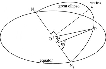
Figure 1.

4. THE GREAT ELLIPTICAL ANGLE-GEA

In Figure 1 a point P is located on the GE at geocentric latitude φ or geodetic latitude ψ and longitude θ. These co-ordinates are omitted for clarity. The point P is also elevated in the plane of the GE to φ′, which is the great elliptical angle (GEA) between a node at longitude θ_n and the point P, i.e. GEA=N₁OP [Reference Walwyn3] [Reference Williams4]. Associated with φ′ is the geodetic angle ψ′. Also at the vertex V, the highest point reached on the GE, the line OV makes a right angle with the equatorial line N₁ O N₂.

In Fig. 2, the GEA of position P₁ is the angle between and defined by:

(5)

for which is the equatorial vector at one of the two nodal points N₁: and are vectors of position for P₁ and P₂ on the GE. In general, a vector has its usual meaning in terms of radius r(φ), latitude φ and longitude θ, namely that . Expanding Equation 5 gives:

(6)

Figure 2.

In Equation 6, φ₁ and θ₁ are the geocentric latitude and the longitude co-ordinates of P₁ and θ_n is the longitude of the node. However Equation 6 is only useful when it is necessary to compute intermediate positions along the GE and is not required for the error analysis to follow.

5. DISTANCE ON THE GE AND GC

Equation 3 gives distance to good accuracy when ε and ψ are replaced with ε′ and ψ′. The GED between two points at P₁, P₂ can then be expressed as:

(7)

After applying Equation 3 and manipulating further:

(8)

where the constant 1·0018 has been included to convert from geodetic to nautical miles.

Since GC latitude angles (φ) on the navigation sphere are both geodetic and geocentric, the sphere can be considered as a degenerated spheroid for which ε=0, hence when computing GCD, angle φ′ can be replaced with ψ′ with no loss of generality i.e.

(9)

(10)

6. ERROR ANALYSIS

Inserting Equation 8 and Equation 10 in Equation 1 the fractional error becomes:

(11)

It is convenient to consider elliptical angles such that their span is centred upon a median value , then on further substituting Equation 4 into Equation 11 we arrive at:

(12)

Median elliptical angle depends upon the latitude ψ and longitude θ in such a way that as it moves along the GE from node it attains the value when the latitude has reached the vertex ψ_v. For the purpose of this analysis however, latitude and longitude of a point on the GE are not required. It is sufficient to recognize that for the range of latitude 0<φ⩽φ_v that and that and φ_v are independent variables.

Equation 12 shows that the largest errors occur for small δ′ so we can allow δ′→0 hence . Then at , the error is:

(13)

which is also identifiable in terms of vertex radius r_v as:

(14)

and has a minimum of 0·18% when φ_v→0 and a maximum of −0·49% for . Also, for and , then η=0·51%. Additional numerical evaluation shows that for other values of φ_v and within these limits and especially about the usual limiting navigation latitudes, the errors are less and we may conclude that overall, GC distances on the navigation sphere in round numbers, are within 0·5% of GE distances on the WGS84 spheroid. Solutions to Equation 12 are shown in Figure 3 which is labeled with error extremes and contours at intervals of 0·1%.

Figure 3.

7. RHUMBLINE COMPARISONS

Analysis of the length of the rhumbline on the navigation sphere between specific points is readily compared to the corresponding length on the spheroid between the same points. The rhumbline distance d₁ on the sphere between defined positions is given by d₁=DLAT sec γ where DLAT is the difference in latitude between two points in n.m, while on the spheroid, the corresponding distance is d₂=1·0018DLP sec γ where DLP is the number of latitude parts on the spheroid separating the same two points. The coefficient 1·0018 converts the DLP in geodetic miles on the spheroid to nautical miles and γ is the azimuth angle. The ratio of these two measures is d₁/d₂ and the fractional error is or:

(15)

which is independent of γ.

On the navigation sphere, DLAT is simply a(φ₂−φ₁) and DLP=L(ψ₂)−L(ψ₁). We then have:

(16)

As before, latitude φ can be replaced with ψ with no loss of generality and with ε=0·08181919 (WGS84) Equation 16 becomes:

(17)

which reduces approximately to:

(18)

From an inspection of Equation 18, the greater values of the fractional error occur for small distances i.e. when . Maximum errors occur for with values very close to ±0·005 or ±0·5% respectively. For moderate values of δ the error is less. As ψ₀ approaches middle latitudes the error diminishes approaching zero at . Elsewhere for other valid values of δ in the range , the distance for a rhumbline on the navigation sphere is within 0·5% of the distance on the rhumbline on the WGS84 spheroid.