


1. Introduction
The problem considered here is that of inferring genetic values and of predicting phenotypes for a quantitative trait under complex forms of gene action, an issue of importance in animal and plant breeding, and in evolutionary quantitative genetics (Lynch & Walsh, Reference Lynch and Walsh1998). The discussion is streamlined as follows. Current methods for dealing with epistatic variability via variance component models are discussed in section 2. Problems posed by cryptic, non-linear, forms of epistasis are identified in section 3. Section 4 proposes non-parametric definitions of additive effects (breeding values), with and without employing molecular information, and shows how these could be inferred using reproducing kernel Hilbert spaces (RKHS) regression models. Sections 5 and 6 present stylized examples to demonstrate the methods. The first example uses the infinitesimal model of quantitative genetics, and the second one tackles a non-linear genetic system. The paper ends with concluding comments.
2. Extant theory
A standard decomposition of phenotypic value in quantitative genetics (Falconer & Mackay, Reference Falconer and Mackay1996) is
where a, d and i are additive, dominance and epistatic effects, respectively, and e is a residual, reflecting environmental (residual) variability. This linear decomposition can also be used to describe variability of latent variables, especially if assumed Gaussian (e.g. Dempster & Lerner, Reference Dempster and Lerner1950; Gianola, Reference Gianola1982). The i effect can be decomposed into additive×additive, additive×dominance, dominance×dominance, etc., deviates. In what has been termed ‘statistical epistasis’ (Cheverud & Routman, Reference Cheverud and Routman1995), these deviates are assumed to be random draws from some distributions representing ‘interactions’ between loci. Under certain assumptions (Cockerham, Reference Cockerham1954; Kempthorne, Reference Kempthorne1954), the deviates are uncorrelated, leading to the standard variance decomposition σ2=σa2+σd2+σaa2+σad2+σdd2+…+σe2, where the σ2s are variance components, e.g., σad2 represents the contribution of additive by dominance effects to variance. The sum of all variance components other than σa2, σd2 and σe2 is interpreted as variance ‘due to epistasis’. For the purposes of discussing problems this representation has, it suffices to assume that the only relevant epistatic effects are those of an additive×additive, additive×dominance and dominance×dominance nature.
(i) Henderson's methods for predicting epistatic effects
Using the Cockerham–Kempthorne (hereinafter, CK) assumptions, Henderson (Reference Henderson1985) extended their model to the infinitesimal domain, and vectorially, by writing
where β is some nuisance location vector (equal to μ if it contains a single element); X is a known incidence matrix; a and d are vectors of additive and dominance effects, respectively; iaa, iad and idd are epistatic effects, and g=a+d+iaa+iad+idd is the ‘total’ genetic value. Assuming that g and e are uncorrelated, the variance–covariance decomposition is
where Vy,Vg and Ve are the phenotypic, genetic and residual variance–covariance matrices, respectively. Further,
Here, A is the numerator relationship matrix; D is a matrix due to dominance relationships which can be computed from entries in A, and the remaining matrices involve Hadamard (element by element) products of matrices A or D. Thus, under CK, all matrices can be computed from elements of A, as noted by Henderson (Reference Henderson1985), because absence of inbreeding and of linkage disequilibrium are assumed. Cockerham (Reference Cockerham1956) and Schnell (Reference Schnell, Hanson and Robinson1963) gave formulae for covariances between relatives in the presence of linkage, and difficulties posed by linkage disequilibrium are discussed by Gallais (Reference Gallais1974).
In CK–Henderson, with the extra assumption that all genetic effects (having null means) and the data (with mean vector Xβ) follow a multivariate normal distribution with known dispersion components, one has
The best predictor (Henderson, Reference Henderson1973; Bulmer, Reference Bulmer1980) of additive genetic value in the mean-squared error sense is
where E g|y (g)=VgVy−1 (y−Xβ) is the best predictor of g, and the matrix of regression coefficients VgVy−1 is the multidimensional counterpart of heritability in the broad sense. With known variance components, β is typically estimated by generalized least-squares (equivalently, by maximum likelihood under normality) as ![]() . Then, ‘the empirical best predictor’ of the vector of additive effects is taken to be
. Then, ‘the empirical best predictor’ of the vector of additive effects is taken to be
This is precisely the best linear unbiased predictor (BLUP) of additive merit when model (1) holds. Likewise, the BLUP of additive×dominance deviations is
and so on.
The BLUPs of a, d, iaa, iad and idd in (1) can be computed simultaneously using Henderson's mixed model equations, but this requires forming the inverse matrices A−1, D−1, (A#A)−1, (A#D)−1 and (D#D)−1. In a general setting, most of these inverses are impossible to obtain, contrary to that of A, which can be written directly from a genealogy.
(ii) Reformulation of Henderson's approach
Equivalently, as in de los Campos et al. (Reference de los Campos, Gianola and Rosa2008), one may rewrite (1) as
where a*=A−1a~(0, A−1σa2),…, idd*=(D#D)−1idd~(0, (D#D)−1σdd2). Then, the BLUP of any of the transformed genetic effects can be found by solving a system of mixed linear model equations that does not involve inverses of any of the genetic variance–covariance matrices. For example, the β-equation is
and the iaa-equation is
Once the BLUPs of the (∗) genetic effects are obtained, linear invariance leads, for example, to ![]() , and to
, and to ![]() . A computational difficulty here is that A is typically not sparse, so all A#A, A#D, etc., are not sparse either. Note that the equations for the genetic effects in the ‘reparameterized’ model are similar to those in Henderson (Reference Henderson1984). For example, if in an animal model the a-equation
. A computational difficulty here is that A is typically not sparse, so all A#A, A#D, etc., are not sparse either. Note that the equations for the genetic effects in the ‘reparameterized’ model are similar to those in Henderson (Reference Henderson1984). For example, if in an animal model the a-equation
is premultiplied by A, one obtains
(iii) Bayesian implementation of the reformulated model
In the standard Bayesian linear model (Wang et al., Reference Wang, Rutledge and Gianola1993, Reference Wang, Rutledge and Gianola1994; Sorensen & Gianola, Reference Sorensen and Gianola2002), ![]() , etc., are mean vectors of corresponding conditional posterior distributions, for which sampling procedures are well known. Further, with scaled inverse chi-square priors assigned to variance components, Gibbs sampling is straightforward, and does not require forming inverses either. For example, a draw from the conditional posterior distribution of the dominance×dominance variance component is obtained under the alternative parameterization as
, etc., are mean vectors of corresponding conditional posterior distributions, for which sampling procedures are well known. Further, with scaled inverse chi-square priors assigned to variance components, Gibbs sampling is straightforward, and does not require forming inverses either. For example, a draw from the conditional posterior distribution of the dominance×dominance variance component is obtained under the alternative parameterization as
where idd* is a draw from its conditional posterior distribution, given everything else (Sorensen & Gianola, Reference Sorensen and Gianola2002) and νdd and S dd2 are hyper-parameters.
While computations may still be formidable, inversion of the genetic covariance matrices is circumvented. Apart from computational issues, an important question, however, is whether or not the CK–Henderson construct can cope with complex genetic systems effectively.
3. Confronting complexity
Dealing with non-additive genetic variability may be much more difficult than what equations (1) and (3) suggest. Theoretically, at least in CK, epistatic variance can be partitioned into orthogonal additive×additive, additive×dominance, dominance×dominance, etc., variance components, only under idealized conditions. These include linkage equilibrium, absence of mutation and of selection, and no inbreeding or assortative mating (Cockerham, Reference Cockerham1954; Kempthorne, Reference Kempthorne1954). All these assumptions are violated in mature and in breeding programmes. Also, estimation of non-additive components of variance is very difficult, even under standard assumptions (Chang, Reference Chang1988), leading to imprecise inference. Linkage disequilibrium induces covariances between different types of effects; algebraically heroic attempts to deal with this problem are in Weir & Cockerham (Reference Weir and Cockerham1977) and Wang & Zeng (Reference Wang and Zeng2006). Gallais (Reference Gallais1974) derived expressions aimed to describe the impact of linkage disequilibrium on partition of genetic variance. The number of parameters is large, which makes estimation of the needed dispersion components intractable.
The question of whether or not standard random effects models for quantitative traits can account accurately for non-linear (non-additive) relationships between infinitesimal genotypes and phenotypes remains open. It is argued subsequently that parametric models cannot handle well complexity resulting from interactions between the hundreds or even thousands of genes expected to affect multifactorial traits, such as liability or resistance to disease. This was discussed by Templeton (Reference Templeton, Wolf, Brodie and Wade2000), Gianola et al. (Reference Gianola, Fernando and Stella2006) and Gianola and van Kaam (Reference Gianola and van Kaam2008).
In the standard theory for non-additive gene action, e.g. epistasis, interaction effects enter linearly into the phenotype, that is, the partial derivative of the model with respect to any effect, be it additive or of an interactive nature, is a constant that does not involve any genetic effect. This theory is unrealistic in non-linear systems, such as those used in metabolic control theory (Bost et al., Reference Bost, Dillmann and De Vienne1999). Arguing from the perspective of ‘perturbation in analysis’, Feldman & Lewontin (Reference Feldman and Lewontin1975) advanced the argument that linear (i.e. analysis of variance) models are ‘local’, presumably in the following sense. Suppose that the expected value of phenotype y, given some genetic values G (genotypes are discrete but their effects are continous), is some unknown function of effects of genotypes at L loci represented as f(G 1, G 2, …, G L). A second-order approximation to the surface of means yields
where ![]() is the mean value of the effect of locus i (typically taken to be 0); G=(G 1, G 2, …, G L)′ is a column vector and Ḡ=E(G); f′(
is the mean value of the effect of locus i (typically taken to be 0); G=(G 1, G 2, …, G L)′ is a column vector and Ḡ=E(G); f′(![]() ) is the row vector of first derivatives of f(.) with respect to G and
) is the row vector of first derivatives of f(.) with respect to G and
is the matrix of second derivatives, both evaluated at Ḡ in the approximation.
A linear-on-variance-components decomposition of variability may not be enlightening at all when a phenotype results, say, from a sum of sine and cosine waves. To illustrate, suppose that non-linearity (non-additivity) enters as E (y|G 1, G 2, G 3)=G 1 exp (G 2G 3). A log-transformation of the expected phenotypic value of individuals with genetic value (G 1, G 2, G 3) would suggest linearity (in a log-scale) with respect to locus 1, and interaction between loci 2 and 3. For this hypothetical model, the first derivatives are

and the matrix of second derivatives is

In the neighbourhood of 0 for all effects, the local approximation yields
On the other hand, near 1 the local approximation produces
A local approximation near 0 suggests that phenotypes are linear on the effect of locus 1, while an approximation in the neighbourhood of 1 points towards ‘dominance’ at loci 2 and 3, and at 2 – factor epistasis involving loci (1, 2), (1, 3) and (2, 3). This relates to work by Kojima (Reference Kojima1959), who studied conditions for equilibria when a fitness surface was affected by epistasis. He assumed free recombination, random mating and constancy of genotypic values. The arguments leading to (8) and (9) indicate that constancy of genotypic values is not tenable when local approximations are used to study the surface.
To the extent that a linear model provides a ‘local’ approximation only, it may not be surprising why attaining an understanding of epistasis within the classical paradigm has been elusive. Kempthorne (Reference Kempthorne1978) disagrees with this view, however, although his argument seems more a defence of the technique of the analysis of variance (ANOVA) per se than of the lack of ability of a linear model to describe complex, interacting, systems. However, even if a linear model holds at least locally, a standard fixed effects ANOVA of a highly dimensional, multifactorial system is not feasible, because one ‘runs out’ of degrees of freedom (df) (Gianola et al., Reference Gianola, Fernando and Stella2006). Nevertheless, methodologies for dealing with complex epistatic systems are becoming available and these include, for example, machine learning, regularized neural networks (Lee, Reference Lee2004), neural networks optimized with grammatical evolution computations (Motsinger-Reif et al., Reference Motsinger-Reif, Dudek, Hahn and Ritchie2008) and non-parametric regression (e.g. Gianola et al., Reference Gianola, Fernando and Stella2006; Gianola & van Kaam, Reference Gianola and van Kaam2008). The latter is discussed in what follows.
4. Non-parametric breeding value
There is a wide collection of procedures for non-parametric regression available. In particular, statistical models based on RKHS have been useful, inter alia, for regression (Wahba, Reference Wahba1990) and classification (Vapnik, Reference Vapnik1998). In many respects, RKHS regression is the ‘mother’ of non-parametric functional data analysis, since it includes splines, hard and soft classification and even best linear unbiased prediction (de los Campos et al., Reference de los Campos, Gianola and Rosa2008) as special cases. Contrary to many ad-hoc forms of non-parametric modelling, RKHS is a variational method based on maximizing penalized likelihoods over a rich space of functions defined on a Hilbert space. Also, it uses flexible kernels, which can be adapted to many different circumstances, and allows for varying classes of information inputs, e.g. pedigrees, continuous valued covariates and molecular markers of any type. The Bayesian view of RKHS regression has been used to motivate the methodology using Gaussian processes (Rasmussen & Williams, Reference Rasmussen and Williams2006). In quantitative genetics, Gianola et al. (Reference Gianola, Fernando and Stella2006) and Gianola & van Kaam (Reference Gianola and van Kaam2008) suggested this approach for incorporating information on dense whole-genome markers into models for prediction of genetic value of animals or plants for quantitative traits. The dense molecular data (e.g. SNPs) enter as covariates into a kernel (incidence) square matrix whose dimension is equal to the number of individuals with genotype information available. Thus, the dimensionality of the problem is reduced drastically, from that given by the number of SNPs to the number of individuals genotyped, typically much lower. González-Recio et al. (Reference González-Recio, Gianola, Long, Weigel, Rosa and Avendaño2008a, Reference Gonzalez-Recio, Gianola, Rosa, Weigel and Avendañob) present applications to mortality rate and feed conversion efficiency in broilers. In the absence of kernels based on substantive theory, genetic interactions are dealt with in RKHS in some form of ‘black box’. However, the focus of non-parametric regression is prediction rather than inference, an issue that will be emphasized in this paper. Relationships between RKHS regression and classical models of quantitative genetics are discussed by de los Campos et al. (Reference de los Campos, Gianola and Rosa2008). A question that arises naturally in plant and animal breeding is whether or not measures of breeding value can be derived from an RKHS regression model.
Briefly, a RKHS regression can be represented in terms of the linear model
where Xβ is as before; Kh={k(xi, xj, h)} is an n×n symmetric positive-definite matrix of kernel entries dependent on covariates (e.g. SNPs) xi and xj (subscripts i and j define the individual whose phenotype is considered and some other individual in the sample, respectively), and possibly on a set of bandwith parameters h which must be tuned in some manner, as noted below. González-Recio et al. (Reference González-Recio, Gianola, Long, Weigel, Rosa and Avendaño2008a) discuss kernels that do not involve any h. Further, α in (10) is a set of non-parametric regression coefficients, one for each individual in the sample of data. For instance, if SNP genotypes enter into k(xi, xj, h), then Khα can be construed as a vector of genetic effects marked by SNPs.
The choice of kernel k (xi, xj, h) is absolutely critical for attaining good predictions in RKHS regression, and it can be addressed via some suitable model comparison, e.g. by cross-validation. Each kernel is associated with a space of functions, and de los Campos et al. (Reference de los Campos, Gianola and Rosa2008) describe conditions under which a kernel may be expected to work well. For example, if a Hilbert space of functions associated with a given kernel spans functions of additive and non-additive genetic effects, the model would be expected to capture such effects. Otherwise, predictions may be very poor, even worse than those attained with a linear model (which, in some cases will also be a RKHS regression).
It can be shown that the solution to the RKHS regression problem is obtained by assuming that α~N(0, Kh−1σα2), where σα2 is a variance component entering into the smoothing parameter ![]() , and by solving
, and by solving

The method can be implemented in either a BLUP – residual maximum likelihood (REML) context, given h assessed previously by cross-validation or generalized cross-validation (Craven & Wahba, Reference Craven and Wahba1979), or in a fully Bayesian manner, with all parameters assigned prior distributions.
The predicted genetic or genomic value is then Khᾶ, as illustrated by González-Recio et al. (Reference González-Recio, Gianola, Long, Weigel, Rosa and Avendaño2008a) in an analysis of broiler mortality in which sires had been genotyped for thousands of SNPs, and by González-Recio et al. (Reference Gonzalez-Recio, Gianola, Rosa, Weigel and Avendaño2008b) in a similar study of food conversion ratio conducted in the same population. Their results suggest that RKHS regression using SNP information can produce more reliable prediction of current and future (offspring) phenotypes than the standard parametric additive model used in animal breeding. Also, albeit not unambiguously, some RKHS specifications with filtered SNPs tended to outperform parametric Bayesian regression models in which additive effects of all SNPs had been fitted.
In what follows, the RKHS machinery is used to develop non-parametric measures of breeding value.
(i) Infinitesimal non-parametric breeding value
Assume that some kernel matrix Kh has been found satisfactory, in the sense mentioned above. Given the context, vector Khα in (10) is a molecularly marked counterpart of g=a+d+iaa+iad+idd in (1). Consider now the positive-definite kernel matrix K=A+D+(A#A)+(A#D)+(D#D). This is positive-definite, because it consists of the sum of positive-definite matrices, and leads to the RKHS model
with α~N(0, K−1 σα2). Here, K does not depend on any bandwidth parameters, which simplifies matters greatly, relative to the parametric specification (7), in which 6 variance components enter into the problem. To obtain the RKHS predictor of genetic value (and with only 2 variance components intervening), note that solving (11) is equivalent to solving
and the genetic value is predicted as
Here, the ‘non-parametric’ breeding value would be Aα, and its predictor is Aᾶ. The posterior distribution of Aα can be arrived at by drawing samples from the posterior distribution of α.
(ii) SNP-based non-parametric breeding value
Let now Kh be a kernel matrix whose entries depend on a string x of SNP genotypes or haplotypes available for a set of individuals having phenotypic records. For example, Gianola & van Kaam (Reference Gianola and van Kaam2008) consider the Gaussian kernel
Alternatively, one could use as kernel
where xjk is the SNP string for chromosome k in individual j, and h 1, h 2, … , h k are chromosome-specific positive bandwidth parameters.
Irrespective of the kernel adopted, let now
where aK is defined as non-parametric breeding value, and γ is independent of aK. With A being the numerator relationship matrix between the individuals having SNP information, use of the reasoning leading to (4) produces
where σa2 is some estimate of additive genetic variance for the trait in question. Thus, the non-parametric breeding value of individual i in the sample has the form
so that, if individuals are unrelated, ![]() , with variance
, with variance ![]() , where kii is the ith diagonal element of K−1.
, where kii is the ith diagonal element of K−1.
Note that
This is equal to Aσa 2 only if K=A and σα2=σa2; in this case, no molecular information is used at all. Suppose now that A=I, so that individuals are genetically unrelated. However, non-parametric breeding values turn out to be correlated, since
This can be interpreted in the following manner, using a Gaussian kernel to illustrate. Here, the entries of the kernel matrix have the form
and ![]() is maximum when xik=xjk, that is, when individuals i and j have the same genotype at marker k. This means that the elements of the kernel matrix (taking values between 0 and 1) will be larger for pairs of individuals that are more ‘molecularly alike’, even if unrelated by line of descent. This molecular similarity is then propagated into (16) and (17).
is maximum when xik=xjk, that is, when individuals i and j have the same genotype at marker k. This means that the elements of the kernel matrix (taking values between 0 and 1) will be larger for pairs of individuals that are more ‘molecularly alike’, even if unrelated by line of descent. This molecular similarity is then propagated into (16) and (17).
Given a point estimate of α(ᾶ), e.g. the posterior mean, the non-parametric estimate of breeding value is
If computations are carried out in a fully Bayesian Monte Carlo context (with m samples drawn from the posterior distribution), the posterior mean estimate is
and the uncertainty measure (akin to prediction error variance–covariance in BLUP) is
Non-parametric breeding values of individuals that are not genotyped can be inferred as follows. Let A(−,+) be the additive relationship matrix between individuals that are not genotyped (−) and those which are genotyped (+). The non-parametric breeding value of non-genotyped individuals would be
with its point estimate being
Likewise, non-parametric breeding values of yet-to-be genotyped and phenotyped progeny would be
where A(prog,+) is the additive relationship matrix between progenies and individuals with data.
(iii) Semi-parametric breeding value
Another possibility consists of treating additive genetic effects in a parametric manner and non-additive effects in the RKHS framework, as suggested by Gianola et al. (Reference Gianola, Fernando and Stella2006). Let now the model be
where u~(0, Aσa2) and Kα as before, but with
where Kh is a positive-definite matrix of Gaussian kernels with entries as in (14), so that SNP information is used. Since K is the sum of Hadamard products of positive-definite matrices, it is positive-definite as well and, hence, it is a valid kernel for RKHS regression. The estimating equations (can be rendered symmetric by premultiplying the α-set of equations by K) take now the form
where û is the predicted breeding value, and
is the predicted (SNP-based) non-additive genetic value. For instance, (D#Kh)ᾶ is interpretable as a predicted dominance value, and so on. A natural extension of this consists of removing u from (19) and then taking as kernel matrix
so that the predicted additive breeding value would now be (A#Kh)ᾶ, much along the lines of (18). This would give a completely non-parametric treatment of prediction of additive and non-additive genetic effects using dense molecular information.
5. Illustration: infinitesimal model
The toy example in Henderson (Reference Henderson1985) is considered. The problem is to infer additive and dominance genetic effects of five individuals using data consisting of phenotypic records for only four (subject 1 lacks a record). The data and model are:

Although 1 does not have a record, all additive and dominance effects are included in the model, zeroing out the incidence of a 1 and d 1 via a column of 0s in the Z incidence matrix. Henderson (Reference Henderson1985) assumed that the additive, dominance and residual variance components were σa2=5, σd2=4 and σe2=20, so that the phenotypic variance was 29, and used the additive and dominance relationship matrices
Application of BLUP leads to the unique solutions (rounded at the third decimal)
The predicted total genetic value is ĝ=â+![]() , yielding
, yielding
Alternatively, a RKHS representation as in (12) is used now, with K=A+D as kernel matrix, which does not involve any bandwidth parameters. One has
The RKHS model (using the part of K pertaining to individual with records) is
The value adopted for the sole smoothing parameter is σα2=σa2+σd2=9, and the estimating equation (11) and the solution to the RKHS mixed model equations is
The non-parametric additive genetic effects are inferred using formula (18)

and the non-parametric estimates of dominance effects are
The total genetic value is estimated at

Suppose now that one wishes to predict future performance of these five individuals, and assume that the record of 1 will be made under the same conditions as those for the record of 2, with all conditions remaining the same. The model for future records f is then
for the parametric model, whereas that for the RKHS treatment is
Above M. and θ. denote incidence matrices and regression coefficients, respectively; P and K indicate parametric and RKHS treatments, respectively. Using a standard Bayesian argument (Sorensen & Gianola, Reference Sorensen and Gianola2002), the mean vector and covariance matrix of the predictive distributions are
where C is the corresponding coefficient matrix for each of the procedures; the 5×5 matrix Ifσe2 conveys uncertainty stemming from the fact that the future records (f) have not been realized yet. For the two procedures, means and standard deviations of the predictive distributions are
6. Illustration: non-linear system
(i) Two-locus model
A hypothetical system with two biallelic loci was simulated. It was assumed that phenotypes were generated according to the rule
where αi (βi) and αj (βj) are effects of alleles i and j at the α (β) locus. The system is nonlinear on allelic effects, as indicated by the first derivatives of the conditional expectation function with respect to the αs or βs. For instance,
The α-effects were two random draws from an exponential distribution with mean value equal to 2; the first draw was assigned to allele A and the second to allele a. The βs were drawn from a Weibull (2,1) distribution, having median, mean and mode equal to 0·347, 0·887 and 0·25; the first (second) deviate was the effect of allele B (b). The non-linearity of the system is illustrated in Fig. 1, where the derivative of the model for the expected phenotype with respect to the effect of Weibull allele b is plotted, with all other alleles evaluated at the values drawn. Variation in values of b produces drastic modifications near the origin, but phenotypes are essentially insensitive for b>1·5, even though these values are plausible in the Weibull process hypothesized.
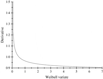
Fig. 1. Rate of change of the expected phenotypic value ![]() with respect to the Weibull variable βj.
with respect to the Weibull variable βj.
Residuals were drawn from the normal distribution N (0, 20), and added to (21) to form phenotypes. The resulting phenotypic distribution is unknown, because y is a non-linear function of exponential and Weibull variates, plus an additive normally distributed residual. There were 5 individuals with records for each of the AABB, AABb, AAbb genotypes; 20 for each of AaBB, AaBb and Aabb and 5 for each of aaBB, aaBb and aabb. Thus, there were 90 individuals with phenotypic records, in total.
Since there are nine distinct mean genotypic values, variation among their average values can be explained completely with a linear model on 9 df; in the standard treatment, these df correspond to an overall mean, additive effects (2 df), dominance (2 df) and epistasis (4 df). Due to non-linearity, it is not straightforward to assess the proportion of variance ‘due to genetic effects’ using a random effects model based on the Weibull and exponential distributions, although an approximation can be arrived at. A linear approximation of the phenotype of an individual yields
where ᾱ and ![]() are the means of the exponential and Weibull processes, respectively, and e~N(0, σ2). An approximation to heritability is
are the means of the exponential and Weibull processes, respectively, and e~N(0, σ2). An approximation to heritability is
For the situation simulated, ྱ = 2, ![]() , Var(α)=4, Var(β)=0·785, so that for σ2=1000, 100, 20, 10 one obtains h 2≈0·13, 0·60, 0·88 and 0·94, respectively. The simulation produced a high penetrance trait, that is, one with heritability near 0·88, which provides a challenge to any non-parametric treatment.
, Var(α)=4, Var(β)=0·785, so that for σ2=1000, 100, 20, 10 one obtains h 2≈0·13, 0·60, 0·88 and 0·94, respectively. The simulation produced a high penetrance trait, that is, one with heritability near 0·88, which provides a challenge to any non-parametric treatment.
(ii) RKHS modelling
Among the many possible candidate kernels available, an arbitrarily chosen Gaussian kernel was adopted for the RKHS regression implementations, using as covariate a 2×1 vector consisting of the number of alleles at each of the two loci, e.g. x AA=2, x Aa=1 and x aa=0. For example, the kernel entry for genotypes AABB and AAbb is

and the 9×9 kernel matrix for all possible genotypes (labels for genotypes are included, to facilitate understanding of entries) is

There are only five distinct entries, a result of the measure of ‘allelic disimilarity’ adopted, e.g. e −8/h stems from disimilarity in 2 alleles at each of the A and B loci (AABB versus aabb). Figures 2 and 3 depict values of the kernel as a function of the bandwidth parameter h at different levels of S, which enters into exp(−S/h). Values of h larger than 10 (Fig. 2) produce strong ‘prior correlations’ between genotypes; also, the kernel matrix becomes more poorly conditioned as h increases. After evaluating the kernel matrix at h=6, 4, 2 and 1·75, it was decided to adopt h=1·75 as the bandwidth parameter, producing 6 unique entries in the K matrix: 1·0 (diagonal elements, the two individuals have identical genotypes); 0·565 (3 alleles in common in a pair of individuals); 0·319 (2 alleles in common, 1 per locus) or 0·102 (2 alleles in common at only one locus); 0·06 (1 allele in common) and 0·01 (no alleles shared).
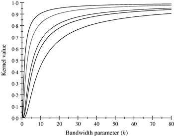
Fig. 2. Kernel value ![]() against the bandwidth parameter h. Curves, from top to bottom, correspond to S=1, 2, 4, 5, 8.
against the bandwidth parameter h. Curves, from top to bottom, correspond to S=1, 2, 4, 5, 8.
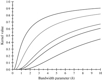
Fig. 3. Kernel value ![]() against the bandwidth parameter h. Curves, from top to bottom, correspond to S=1, 2, 4, 5, 8.
against the bandwidth parameter h. Curves, from top to bottom, correspond to S=1, 2, 4, 5, 8.
(iii) Fitting the RKHS model to the means
A ‘means’ RKHS regression was fitted, including an intercept (β). The model for the 9×1 vector of averages ![]() was
was
where the αs are the non-parametric regression coefficients; K1·75 is the 9×9 kernel matrix with h=1·75 and ![]() is the mean of the residuals pertaining to observations of individuals with genotype i. As before, the assumptions were
is the mean of the residuals pertaining to observations of individuals with genotype i. As before, the assumptions were ![]() , and, for the 9×1 vector of average residuals,
, and, for the 9×1 vector of average residuals, ![]() . Here, N=Diag {5, 5, 5, 20, 20, 20, 5, 5, 5} is a 9×9 diagonal matrix.
. Here, N=Diag {5, 5, 5, 20, 20, 20, 5, 5, 5} is a 9×9 diagonal matrix.
The solution to the RKHS regression problem was obtained as
The model was fitted for each of the following values of the shrinkage ratio ![]() : 100 (strong shrinkage towards 0), 15, 1,
: 100 (strong shrinkage towards 0), 15, 1, ![]() and
and ![]() ; with λ=0 there is no shrinkage of solutions at all. For each of these values, the residual sum of squares
; with λ=0 there is no shrinkage of solutions at all. For each of these values, the residual sum of squares
and the weighted residual sum of squares
were computed, where 1 is a 9×1 vector of ones. Also, the effective number of parameters, or model df (Ruppert et al., Reference Ruppert, Wand and Carroll2003), was assessed as
where
and ![]() is a diagonal matrix containing the square roots of the entries of N. Note that, when
is a diagonal matrix containing the square roots of the entries of N. Note that, when ![]() , the estimating equations have an infinite number of solutions, as only 9 parameters are estimable. In this case, a solution is obtained by using a generalized inverse of the coefficient matrix, yielding
, the estimating equations have an infinite number of solutions, as only 9 parameters are estimable. In this case, a solution is obtained by using a generalized inverse of the coefficient matrix, yielding
Here, the fitted values are ![]() so the model ‘copies’ the data, and the fit is perfect. Note that
so the model ‘copies’ the data, and the fit is perfect. Note that ![]() is the least-squares estimate of μij=γi+δj+(γδ)ij where γi (i=AA, Aa, aa) and δj (j=BB, Bb, bb) are main effects of genotypes at loci A and B, respectively; this model accounts for 8 df ‘due to’ additive and dominance effects at each of the two loci, and additive×additive, additive×dominance, dominance×additive and dominance×dominance interactions.
is the least-squares estimate of μij=γi+δj+(γδ)ij where γi (i=AA, Aa, aa) and δj (j=BB, Bb, bb) are main effects of genotypes at loci A and B, respectively; this model accounts for 8 df ‘due to’ additive and dominance effects at each of the two loci, and additive×additive, additive×dominance, dominance×additive and dominance×dominance interactions.
For the sake of comparison, the following fixed effects model was fitted as well
where, as before, γi (i=AA, Aa, aa) are main effects of genotypes at the A-locus, and δj (j=BB, Bb, bb) are the counterparts at the locus B. The linear model was parameterized as
This model has 5 free parameters, interpretable as an ‘overall mean’ plus additive and dominance effects at each of the 2 loci. Estimates of estimable functions of fixed effects were obtained from a weighted least-squares approach with solution vector ![]() where (X′NX)− is a generalized inverse of X′NX and X is the 9×7 incidence matrix given above. Weighted residual sums of squares were computed as
where (X′NX)− is a generalized inverse of X′NX and X is the 9×7 incidence matrix given above. Weighted residual sums of squares were computed as ![]() . Mean values of A-locus and B-locus genotypes were estimated as
. Mean values of A-locus and B-locus genotypes were estimated as
and dominance effects were inferred as

This analysis would create the illusion of non-additivity and overdominance at the A and B loci, respectively, but without bringing light with respect to the non-linearities of (21). While this model does not have mechanistic relevance, it has predictive value, an issue which is illustrated below.
Table 1 gives estimates of the intercept β and of the RKHS regression coefficients α for each of the shrinkage ratio values employed, using h=1·75 as bandwidth parameter in all cases. The residual sum of squares (weighted and unweighted) and the effective number of parameters, or model df, are presented as well. As λ decreased from 102 to 10−2, model fit improved, but the efective number of parameters increased from 1·46 to 8·95, near the maximum of 9. The implementations with λ=15−1 and λ=10−2 essentially produced a ‘saturated’ model, that is, one that fits to the means perfectly (as it is the case when λ=0). Large values of the variance ratio (15, 100) produced excessive shrinkage, as indicated by the small values of the RKHS regression coefficients α, and small values of the variance ratio tended to overfit, as noted. On the other hand, the linear 2-locus model on additive effects, with 5 parameters, had residual sum of squares, SSR=19·98, and weighted residual sum of squares, SSR=99·88. These values are more than 5 times those attained with the RKHS regression implementation with a variance ratio of 1 (SSR=3·55, WSSR=19·12), which are shown in Table 1.
Table 1. Estimates of the intercept (β) and of non-parametric regression coefficients (αi) for each of the values of the variance ratio (λ=σe2/σα2) employed. RSS and WRSS are the residual and weighted residual sums of squares, respectively; df gives the model df, or effective number of parameters fitted

A more important issue, at least from the perspective taken in this paper, is ‘out of sample’ predictive ability. To examine this, 3 new (independent) samples of phenotypes were generated, assuming the residual distribution N (0, 20), as before, and with 5 individuals per genotype, i.e. there were 45 subjects in each sample. The predictive residual sums of squares (unweighted and weighted, using 5 as weight) were calculated, using the fitted values from the training sample employed to compute statistics in Table 1, and the ‘new sample’ phenotypes. The 2-locus additive model was also involved in the comparison. Results are shown in Table 2, where entries are the average, minimum and maximum values of the predictive sum of squares over the 3 new samples. As expected, predictive residual sum of squares were much larger than those observed in the training sample, notably for implementations in which overfitting to the training data was obvious ![]() see Table 1). The specifications producing strong shrinkage towards 0 in the training sample had the worse predictive performance, whereas that with
see Table 1). The specifications producing strong shrinkage towards 0 in the training sample had the worse predictive performance, whereas that with ![]() had the best performance, on average, albeit close to the 2-locus additive model. It is not surprising that small variance ratios led to reasonable predictive performance, be-cause the simulation mimicked high penetrance, i.e. phenotypes are very informative about genotypes, this being so because the approximate heritability (22) for a residual variance of 20 is about 0·88, as already noted.
had the best performance, on average, albeit close to the 2-locus additive model. It is not surprising that small variance ratios led to reasonable predictive performance, be-cause the simulation mimicked high penetrance, i.e. phenotypes are very informative about genotypes, this being so because the approximate heritability (22) for a residual variance of 20 is about 0·88, as already noted.
Table 2. Predictive (weighted and unweighted by the number of individuals per geno-type) residual sums of squares for each of the variance ratios (λ=σe2/σα2) employed in the non-parametric regression implementation, and for the two-locus model with main effects of genotypes at each of the loci. Entries are average (boldface) from three predictive samples, with minimum and maximum values over samples in parentheses

For this example, the 2-locus additive model is untenable, at least mechanistically, yet it had a reasonable predictive performance. Apart from genetic considerations discussed later, this is because any of the models considered here can be associated with a linear smoother, with predictions having the form
for some matrix L and where li′ is its ith row. For the 2-locus model,
whereas for any of the RKHS specifications
Hence, all predictors can be viewed as consisting of different forms of averaging observations, with the RKHS-based averages having optimality properties, in some well defined sense (Kimeldorf & Wahba, Reference Kimeldorf and Wahba1971; Wahba, Reference Wahba1990; Gianola & van Kaam, Reference Gianola and van Kaam2008; de los Campos et al., Reference de los Campos, Gianola and Rosa2008). Since the data consisted of phenotypic averages, i.e. a non-parametric averaging method where a ‘bin’ is a given genotype, this represented a challenge for any of the smoothers, including the 2-locus additive model. However, some of the smoothers (e.g. RKHS with λ=1 and the 2-locus additive model) met the challenge satisfactorily.
(iv) Fitting the RKHS model to individual observations
The RKHS regression model (using the Gaussian kernel with h=1·75) was fitted again to the 90 data points in a newly simulated sample used to estimate (train) the intercept and the nine non-parametric coefficients. In addition, the following parametric specifications were fitted: additive model (3 location parameters: intercept and additive effects of the A and B loci), additive+dominance model (2 extra parameters corresponding to dominance effects at the two loci), and additive+dominance+epistasis (4 additional df pertaining to additive×additive, additive×dominance, dominance×additive and dominance×dominance interactions). The corresponding regression coefficients for the parametric models were ‘shrunken’ using a common variance ratio, corresponding to each of the 15 λ values employed in the RKHS fitting. Subsequently, 100 predictive samples of size 45 each were simulated, and the realized values were compared against the predictions obtained from the sample used to train either the RKHS regression or the three parametric models.
Figure 4 displays the average squared residual (over the 90 data points in the training sample) for each of the four models fitted. As expected, the RHKS and the additive+dominance+epistatic models fitted the data best at λ=0 (no shrinkage), because of having a larger effective number of parameters (9) than the additive (3) and additive+dominance (5) models. When effects were gradually shrunken (λ increased from 0 to 20), the parametric models maintained their relative standings, whereas RKHS voyaged through all three models, eventually giving a very poor fit, due to oversmoothing. The trajectory of the effective df is shown in Fig. 5, where the ability of RKHS to explore models of different degrees of complexity becomes clear. The out-of-sample predictive performance of the four models is shown in Fig. 6. The simplest model, that is, one with additive effects at each of the two loci fitted, had the best predictive performance, even better than the two additional parametric specifications although the simulated gene action was not additive at all! RKHS regression was competitive, but its predictive ability deteriorated markedly when λ was greater than 5 in the training sample.
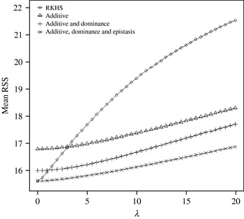
Fig. 4. Average (over 90 data points) squared residual for four models plotted to the training sample (RKHS=RKHS regression with Gaussian kernel and h=1·75) for each value of the smoothing parameter λ.
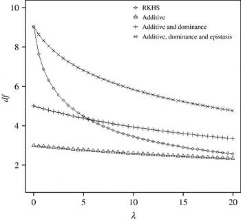
Fig. 5. Effective df for four models plotted to the training sample (RKHS=RKHS regression with Gaussian kernel and h=1·75) at each value of the smoothing parameter λ.
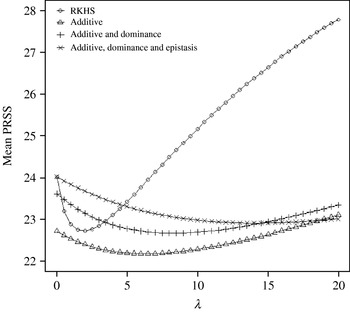
Fig. 6. Average (over 100 samples with 45 realized observations in each) squared prediction error for four models plotted to the predictive sample (RKHS=RKHS regression with Gaussian kernel and h=1·75) for each value of the smoothing parameter λ.
How does one explain the paradox that a simple additive model had better predictive performance when gene action was non-linear, as simulated here? In order to address this question, consider the ‘true’ mean value of the 9 genotypes simulated:
The ‘corrected’ sum of squares among these means is 125·23. A fixed effects ANOVA of these ‘true’ values (assuming genotypes were equally frequent) gives the following partition of sequential sum of squares, apart from rounding errors: (i) additive effect of locus A: 82·8%; (ii) additive effect of locus B after accounting for A: 7·06%; (iii) dominance effects of loci A and B: 4·2%, and (iv) epistasis: 6·2%. Thus, even though the genetic system was non-linear, most of the variation among genotypic means can be accounted for with a linear model on additive effects. The additive model had the worst fit to the data (even worse than the models that assume dominance and epistasis) and, yet, it had the best predictive ability, followed by RKHS for (roughly) 0·5<λ<3.
The simulation was also carried out at larger values of the residual variance, σe2=100 and 500. Again, the purely additive model had the best predictive performance, but the difference between models essentially disappeared for λ>50. In particular, the average squared prediction error of RKHS was larger than that for the additive model by 5, 3 and 1% for σe2=20, 100 and 500, respectively, when evaluated at the ‘optimal’ λ in each case.
It should be noted that the RKHS implementation used here was completely arbitrary. For example, the kernel chosen was not the result of any formal model comparison, so predictive performance could be enhanced by a more judicious choice of kernel. As noted earlier, the choice of a good kernel is critical in this form of non-parametric modelling.
7. Conclusion
Inference about genotypes and future phenotypes for a complex quantitative trait was discussed in this paper. In particular, it was argued that the Kempthorne–Cockerham theory for partioning variance into additive, dominance and epistatic components has doubtful usefulness, because practically all assumptions required are violated in artificial and natural populations. This theory is probably illusory when genetic systems are complex and non-linear, in agreement with views in Feldman & Lewontin (Reference Feldman and Lewontin1975) and Karlin et al. (Reference Karlin, Cameron and Chakraborty1983). Further, an ANOVA-type decomposition is inadequate for a non-linear system (because the ANOVA model is linear in the parameters), and unfeasible in a highly dimensional and interactive genetic system involving hundreds or thousands of genes. As a minimum, the ANOVA treatment would encounter a huge number of empty cells, extreme lack of orthogonality, and high-order interactions would be extremely difficult to interpret, in the usual sense. Last but not the least, the ANOVA model would require more df than the number of data points available for analysis.
For these reasons, a predictive approach was advanced in this paper, focused on the use of non-parametric methods, especifically RKHS regression. Use of this methodogy in conjunction with standard theory of quantitative genetics leads to non-parametric estimates of additive, dominance and epistatic effects. These ideas were illustrated using a stylyzed example in Henderson (Reference Henderson1985), and it was shown how additive, dominance and total genetic values can be predicted using a single smoothing parameter (in addition to the residual variance) coupled with kernels based on substantive theory, a point that is also made in de los Campos et al. (Reference de los Campos, Gianola and Rosa2008). A non-linear 2-locus system was simulated as well, to illustrate the RKHS approach, which was found to have a better out-of-sample predictive performance of means than the standard 2-locus fixed effects model (with and without epistasis).
On the other hand, a 2-locus model with estimates of additive effects shrunken to different degrees had the best performance when predicting future individual observations. This was explained by the observation that most of the variation among genotypic means could be accounted for by ‘additive effects’. This is consistent with theoretical and empirical results presented by Hill et al. (Reference Hill, Goddard and Visscher2008), who gave evidence that, even in the presence of non-additive genetic action, most variance is of an additive type. Even though molecular geneticists view the additive model as irritatingly reductive, our results give reassurance to a common practice in animal breeding, i.e. predict genetic values using additive theory only. It is unknown, however, to what extent these results (from a predictive perspective) carry to more complex systems, difficult to be described suitably with naive linear models. In such situations, RKHS regression could be valuable, because of its ability to navigate through models of different degrees of complexity and, as shown here, it can be very competitive when the smoothing parameters are tuned properly.
In conclusion, it is felt that the non-parametric methods discussed here coupled with machine learning procedures, such as in Long et al. (Reference Long, Gianola, Rosa, Weigel and Avendaño2007) and Long et al. (Reference Long, Gianola, Rosa, Weigel and Avendaño2008), could play an important role in quantitative genetics in the post-genomic era.
Useful comments made by two anonymous reviewers and by Professor William G. Hill and Dr Andres Legarra are acknowledged. Professor Daniel Sorensen is thanked for suggesting that a 2-locus additive model with shrinkage of effects could have good predictive value, which was confirmed. Part of this work was carried out while the senior author was a Visiting Professor at Georg-August-Universität, Göttingen (Alexander von Humboldt Foundation Senior Researcher Award), and Visiting Scientist at the Station d'Amélioration Génétique des Animaux, Centre de Recherche de Toulouse (Chaire D'Excellence Pierre de Fermat, Agence Innovation, Midi-Pyreneés). Support by the Wisconsin Agriculture Experiment Station and by NSF DMS-NSF grant DMS-044371 to the first author is acknowledged.


