


INTRODUCTION
The human microbiota consists of communities of microorganisms that inhabit the human body. These communities can significantly affect many aspects of human physiology. For example, in healthy individuals the microbiota provides a wide range of metabolic functions that humans lack, making their presence advantageous [Reference Gill1, Reference Sommer and Backhed2]. In addition, altered microbial communities are associated with a number of chronic inflammatory disorders including autoimmunity and allergic disorders [Reference Aas, Gessert and Bakken3] as well as, obesity and diabetes [Reference Devaraj, Hemarajata and Versalovic4]. One analytical goal of microbiota studies is to compare the bacterial communities across groups to identify bacteria that either adversely affect or promote health [5].
Altered microbial communities may play an important role in eosinophilic oesophagitis (EoE), which is an allergic inflammatory condition of the oesophagus. A study aimed at better understanding the microbial role of this condition collected samples from the oesophagus and neighbouring nasal and oral cavity sites from subjects with EoE, gastrooesophageal reflux disease (GORD) and with normal mucosa. The original analyses of this study were performed in two parts, first was the comparison of the sample sites in normal subjects [Reference Fillon6] and second was the comparison across the disease groups for a single sample type [Reference Harris7]. A generalized linear mixed model using a distribution appropriate for the characteristics of microbiota data and that includes random effects to account for the within-subject variability is needed to analyse both important questions simultaneously.
Bacteria are generally identified using culturing methods, which assume prior knowledge of the growth condition required for isolation. With the advent of DNA-based sequencing technology, identification of organisms present in the community can now be performed in parallel, which results in significant efficiency compared to culture. The process starts with the collection of human-associated samples for DNA extraction. The DNA is used to amplify 16S rRNA gene sequences that are taxonomically informative, and data are collected using next-generation sequencing technologies. These data are compared to reference databases to determine the identity of an organism (taxonomic category). The number of sequences for a single taxon is then counted for each sample for comparison across groups or conditions.
Microbiota sequence data are high-dimensional with added complexity. They consist of non-negative, highly skewed sequence counts with a large number of zeros. The number of zeros in the dataset is a result of combining samples with different bacterial composition (e.g. disease vs. controls or different locations in one subject). A zero count is inserted for organisms specific to certain groups that are not observed in the samples from the other group. The absence of a count for an organism can be due to the fact that the organism simply is not present in the sample (true zeros) or that the organism is present but undetected (false zeros). In addition, the number of total sequences varies from sample to sample. This is a result of an inability to specify exactly the number of sequences to be measured on a sample using currently available technology. Note the number of sequences obtained is primarily influenced by technical issues with normalizing the concentration of the PCR products from each sample and does not reflect specific biological features of the sample. This attribute of sequencing data requires some consideration as the sequence counts themselves do not correspond to absolute quantities but rather relative quantities with respect to the total number of sequences observed [Reference McMurdie and Holmes8].
Recently, there has been a move towards utilizing models with appropriate distributional assumptions for next-generation sequencing data [Reference McMurdie and Holmes8–Reference Hardcastle and Kelly13]. The negative binomial (NB) distribution has been utilized to model this type of data [Reference Anders and Huber11] and can be written as an extension of Poisson regression, enabling greater flexibility in modelling the relationship between the conditional variance and the conditional mean. However, there can be a lack of fit by the NB due to the excess number of zeros. Recently, a zero-inflated (ZI) gamma distribution has been proposed for the analysis of microbial sequence data in which the excess zero counts are modelled [Reference Paulson9]. Here, we extend these contributions by applying a zero-inflated negative binomial (ZINB) distribution, which is a mixture of a binary distribution that is degenerate at zero and an ordinary count distribution such as NB.
Moreover, often because of a hierarchical study design or data collection, the observations are either clustered or outcomes are collected repeatedly from individual subjects. Few microbiota studies address the within-subject variability attributed to repeated samples collected from a subject, but more recently, authors have begun to utilize methods appropriate for this study design [Reference Smith14, Reference Wu15]. Romero et al. [Reference Romero16] similarly used a ZINB mixed model with a single random effect in the count distribution to model microbiota data. The term mixed is used here to denote models with both fixed and random effects which is a separate concept from the mixture distribution used to describe ZI models. This work proposes the use of a ZINB mixed model, allowing for two random effects, one in the count distribution and one in the ZI component, to compare the relative abundance of two important organisms across disease states and sampling sites in a study of oesophageal microbiota.
METHOD
Motivating example
The dataset is from a study in which paediatric and adult individuals provided samples to capture oesophageal microbiota. The different sample types include the ‘gold standard’ mucosal biopsy [Reference Benitez17] and the minimally invasive capsule-based string collection, the Entero-Test (HDC Corp., USA), named the ‘esophageal string test’ (EST) in that study. Additionally, an oral string segment and nasal cavity swabs were collected for comparison. Of the 70 subjects enrolled in this study, 37 were diagnosed with EoE, eight had GORD and 25 had normal histological biopsy findings. There were 230 samples with adequate bacterial load for data generation from 70 string samples, 30 biopsies and 68 and 62 samples from oral and nasal sites, respectively. Additional details of the study and the data generation process have been previously published [Reference Fillon6, Reference Harris7] and a detailed description of the sequencing methods are given in the Supplementary material. The DNA sequencing data were deposited in the NCBI Short Read Archive database under the accession number SRP041586.
The previous analyses of these data had shown that Haemophilus was significantly elevated in the EoE untreated string samples compared to the normal string samples. Without the use of a model-based approach, it is unclear whether these differences are similarly observed in the other sample types or whether the relative abundance is associated with eosinophil numbers, a marker for disease activity. For the Fusobacterium taxon, differences were observed in string samples collected from subjects residing in the two study locations (Denver, CO and Chicago, IL). It was also noted that the treatment for EoE differed across the study locations, it is unclear whether the difference between the two locations was due to geographical differences or treatment differences. The aim of this analysis is to address these follow-up questions with the application of a ZINB mixed model.
Ethics statement
All human specimens were collected under approval of the Colorado Multiple Institutional Review Board (COMIRB). Written informed consent and HIPAA authorization were obtained from all participants or from parents/legal guardians of participants aged < 18 years. Assent was obtained from all participants aged <18 years.
ZINB mixed model
The ZINB [Reference Greene18, Reference Yau, Wang and Lee19] model assumes there are two distinct data generation processes, determined with the use of a Bernoulli trial. With probability π, the response of the first process is a zero count, and with probability of (1 − π) the response of the second process is governed by a NB with mean λ, which also generates zero counts. The overall probability of zero counts is the combined probability of zeros from the two processes. Thus, a ZINB model for the response Y can be written as:
 $$P\left( {Y = 0} \right) = \; \pi + \left( {1 - \pi} \right)\left( {1 + k\lambda} \right)^{ - \textstyle{1 \over k}}, $$
 $$P\left( {Y = y} \right) = \left( {1 - \pi} \right)\displaystyle{{{\rm \Gamma} \left( {y + \displaystyle{1 \over k}} \right)\left( {k\lambda} \right)^y} \over {{\rm \Gamma} \left( {y + 1} \right){\rm \Gamma} \left( {\displaystyle{1 \over k}} \right)\left( {1 + k\lambda} \right)^{y + \textstyle{1 \over k}}}},$$
where, y = 1, 2, ….
Moghimbeigi et al. [Reference Moghimbeigi20] developed multi-level ZINB regression for modelling overdispersed (where the variance is greater than that expected by the distribution) count data with extra zeros. Allowing Y
ij
(i = 1, 2, … , m; j = 1, 2, … , n
i
and $\mathop \sum \nolimits_{i = 1}^m n_i = n$
gives the total number of observations) to be the response variable for the ith individual subject with jth repeated measurement, a ZINB mixed model is defined as follows:
$\mathop \sum \nolimits_{i = 1}^m n_i = n$
gives the total number of observations) to be the response variable for the ith individual subject with jth repeated measurement, a ZINB mixed model is defined as follows:
 $${\rm log}\left({ {\lambda}_{ij} \vert u_i}\right) = {\bi X}_{\bi ij}^{\prime} {\bi \beta} + u_i,$$
 $${\rm logit}({\pi}_{ij} \vert v_i ) = {\bi Z}_{\bi ij}^{\prime}\gamma + v_i,$$
where X ij and Z ij are vectors of covariates for the NB and the logistic components, respectively, and β and γ are the corresponding vectors of regression coefficients. Note the covariates for the two components are not necessarily the same. Here, u i and v i are the random intercepts and are assumed to be independent and follow the bivariate normal distribution as
 $$\left[ {\matrix{ {u_i} \cr {v_i} \cr } } \right] \sim BVN \left( {\left[ {\matrix{ 0 \cr 0 \cr } } \right],\left[ {\matrix{ {\sigma _u^2 } & 0 \cr 0 & {\sigma _v^2 } \cr } } \right]} \right).$$
For simplicity, we assume the independence of the two random effects, although this is not a necessary assumption, it is commonly used for ZI models with random effects [Reference Hur21, Reference Yau and Lee22] and corresponds with the assumption that the process which generates the false zeros is independent of the process that generates the sequence counts. This assumption was evaluated in a sensitivity analysis with the inclusion of a non-zero correlation between the random effects.
An offset, the natural logarithm of the total sequence counts, log(total ij ), was added to the linear predictor function of the NB component to account for the variable number of sequences per sample inherent in microbiota sequence data. That is,
 $${\rm log}(E(Y_{ij} \vert u_i )) = {\bi X}_{{\bi ij}} {\bi ^{\prime}} + u_i + {\rm log}\left( {{\rm total}_{ij}} \right)$$
can be simplified to show that
 $${\rm log}\; \left( {\displaystyle{{E\left( {Y_{ij}} \right)} \over {{\rm total}_{ij}}} \vert u_i} \right) = {\bi X}_{{\bi ij}} ^{\prime} + u_i. $$
Therefore, the left side of this equation is modelling the log of the relative abundance as the outcome, assuming the total sequence count is considered a fixed value rather than a random variable. Note that the parameter π ij is not affected by the total sequence count.
A ZINB mixed model was applied separately to two organisms identified in the flagship papers (Haemophilus and Fusobacterium) to compare across-disease status and different sample types from the motivating dataset. Variables were included in the model based on a priori decisions of the question of interest and potential confounders of that question. Not all the variables included in the count part of the model were also included in the ZI part of the model for simplification, details are denoted in the results.
Point estimates and P values for the differences between disease status and sample types (EST, biopsy, nasal and oral) were calculated using linear contrasts of the regression parameters. All analyses were performed via the nlmixed procedure using SAS v. 9.3 software (SAS Institute Inc., USA). A two-sided P value <0·05 was considered statistically significant. All corresponding codes used for analysis are included in the Supplementary material.
RESULTS
We demonstrate the application of the ZINB mixed-effects regression model to two organisms identified in the flagship paper [Reference Harris7]. These organisms represent different distributions with different proportions of observed zero counts (Fig. 1).
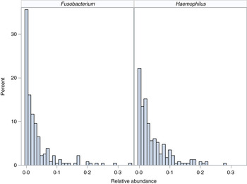
Fig. 1. Distribution of organisms. Histograms for relative abundance measures for Fusobacterium (left) and Haemophilus (right) are displayed for all collected samples.
Haemophilus
The count part of the model for Haemophilus included variables denoting sample type, treatment, diagnosis, indicator for active disease and interactions of EoE diagnosis by proton pump inhibitor (PPI) treatment and EoE diagnosis by sample type. Total sequence count and GORD diagnosis were included in the ZI part of the model, sample type and EoE diagnosis were tested but removed for non-significance. The parameter estimates from the ZINB mixed model are displayed in Table 1. This model contains the total sequence count in both components, as an offset in the count distribution and as a predictor with a parameter estimate in the ZI component. The positive parameter estimate for this variable in the ZI part of the model indicates that as more information is known (i.e. more total sequences are obtained for a sample), the probability that the zero count originates from the ZI component increases. The significance of the overdispersion (OD) parameter indicates the use of the NB distribution over the Poisson distribution is warranted. The likelihood ratio test (LRT) comparing the ZINB model to the nested NB model was significant (χ 2 = 13.0, d.f. = 4, P = 0.01), illustrating the ZI model provided better fit. Active disease as indicated by eosinophil numbers >15 was not significant. The relative abundance of Haemophilus in the string samples from untreated EoE subjects was 7·4% compared to 3·5% in normal subjects (P = 0·01). Similar results were observed in the biopsy samples (6·7% vs. 3·6%) but were only marginally different (P = 0·05), likely due to the smaller number of biopsy samples available for analysis. Oral samples had a higher relative abundance of Haemophilus and nasal samples had lower relative abundance compared to string samples (Fig. 2).

Fig. 2. Least square mean estimates (points) and corresponding 95% confidence intervals (whiskers) of Haemophilus relative abundance by eosinophilic oesophagitis (EoE) diagnosis across anatomical sites.
Table 1. ZINB model parameters for Haemophilus

ZINB, Zero-inflated negative binomial; CI, confidence interval; PPI, proton pump inhibitor; GORD, gastro-oesophageal reflux disease; EoE, eosinophilic oesophagitis.
Both of the variances for the random effects were significant, there was more subject-level variability in the ZI part of the model. The variance of the random effect for the ZI part of the model, v i , was significant, indicating that the probability of a false zero count was different in the subjects. The random-effect variance for the count distribution, u i , was also significant, meaning that some subjects had higher sequence counts compared to others. As a sensitivity analysis, a model that included correlation between random effects was estimated. This correlation was not significant (P = 0·72), thus providing no evidence that the two processes (false zeros and the count process) can be considered dependent.
Fusobacterium
To address the follow-up questions for the Fusobacterium organism, we fitted a ZINB model to all but the biopsy samples, as these were not collected from the Illinois location. The count part of the model included variables denoting EoE diagnosis, sample type, steroid treatment, study location, and a steroid treatment × study location interaction. EoE diagnosis, PPI treatment and study location were included in the ZI part of the model. The parameter estimates from the ZINB mixed model are displayed in Table 2. The significance of the OD parameter indicates the use of the NB distribution over the Poisson distribution is warranted. The LRT comparing the ZINB model to the nested NB model was significant (χ 2 = 14.1, d.f. = 4, P = 0.01), illustrating the ZI model provided better fit. There was a difference in the relative abundance between nasal and oral sites (P < 0·01) and between nasal and string sites (P < 0·01) but not between oral and string sites (P = 0·53). The steroid treatment × study location interaction was significant (P = 0·04). The least square means corresponding to this interaction for the string samples are displayed in Figure 3. The relative abundance of Fusobacterium was not different for subjects not on steroid treatment between the two study locations (P = 0·11) but was different for those on steroid treatment (P < 0·01). There was a marginally significant difference between those on steroid treatment and those who were not at the Chicago location (P = 0·06), a similar difference was not observed for the Denver location (P = 0·38). Only the variance for the random effect for the count distribution was significant indicating that some subjects had higher sequence counts compared to others. The variance for the random effect in the ZI model was estimated to be zero so this effect was removed from the final model.

Fig. 3. Least square mean estimates (points) and corresponding 95% confidence intervals (whiskers) of study location and steroid treatment for Fusobacterium in string samples.
Table 2. ZINB model parameters for Fusobacterium

ZINB, Zero-inflated negative binomial; CI, confidence interval; EoE, eosinophilic oesophagitis; PPI, proton pump inhibitor.
DISCUSSION
This work illustrates the application of a ZINB mixed model approach to a motivating example which included 16S sequence counts for two bacterial organisms with multiple measurements from different anatomical sites. Here, we demonstrate the application and usefulness of the model which is capable of addressing the unique characteristics of microbiota data.
The use of the ZINB mixed model approach allowed the analysis of the motivating dataset within a single model which is in contrast to the two separate analyses performed for the two flagship papers [Reference Fillon6, Reference Harris7]. With the ZINB mixed model, we similarly found that Haemophilus was elevated in untreated EoE compared to normal in the string samples. However, with the model-based approach we were also able to determine this difference was also present in the other sample types. Additionally, information related to the within-subject variability across the repeated sample sites was obtained, both random effects were significant and there was more variability estimated for the ZI component of the model. For the Fusobacterium organism, we similarly found the difference in the relative abundance across study geographical locations were attributable to an interaction between location and steroid treatment with the model-based approach. The difference observed previously between the nasal and string sites in healthy subjects was confirmed in this analysis. Although, in this analysis, we also determined that this difference remained significant when compared across all subjects, including EoE and subjects receiving PPI or steroids, suggesting that Fusobacterium distinguishes these sites despite disease or treatment.
The authors note that a similar approach using a ZINB distribution has been previously applied to microbial sequence data [Reference Romero16]. These authors applied three distributions to over 25 organisms, they found that the majority of the organisms had overdispersion making the Poisson distribution an unreasonable choice and that roughly 25% of the organisms had better fit by the ZINB model over the NB. For the two organisms investigated here, we similarly found that the overdispersion parameter was significant and that the ZINB model fitted better than the NB model. The models in Romero et al. [Reference Romero16] included only a single random effect for the count distribution whereas in our model for Haemophilus, we found significant random effects for both the count and the ZI component of the model. The use of a ZI gamma model has also been recently proposed [Reference Paulson9], while our approach similarly utilizes the ZI mixture to account for excess zeros, it differs in two ways. First, the count process is modelled using a NB in lieu of the gamma. The use of a NB with the variable sequencing effort as an offset has recently been advocated as an alternative to modelling a relative abundance transformation [Reference McMurdie and Holmes8]. Second, our motivating example includes multiple samples collected from a subject which necessarily requires the estimation of within-subject variability with the inclusion of random effects in the model.
ZI models have additional parameters which may require larger sample sizes to obtain adequate estimates. The need for the added complexity should be compared and tested with a simpler model. For both of the example taxa investigated here, the ZINB model provided better fit over the NB model as indicated by the LRT. Moreover, we illustrate the application of the more complex ZINB model to a dataset with a modest sample size.
Although, the use of this model-based approach is an improvement upon the usual simple two-group comparisons, it is not without its limitations. In this work, we chose to focus on the two organisms that were identified in our previous analyses. However, given that microbiota data are high-dimensional, the feasibility of a model applied to more organisms is worth some discussion. The two organisms chosen for inclusion in this analysis did represent a range of potential distributions indicating that the proposed model could also be applied to organisms with distributions within this range. However, these complex ZINB models may not converge when sparseness in the count distribution is present with too few non-zero counts. For high-dimensional applications, it may be possible to use simpler models for individual taxa when the ZI model may not outperform a simpler count distribution or to borrow information across taxa for certain parameters. In such a case, adjustments for multiple comparisons would also need to be considered. It is more likely that this ZINB mixed model will be useful for addressing more focused questions related to a small subset of organisms of clinical interest as was proposed here.
The distributions of the microbial sequence counts are complex, often containing highly skewed, non-negative values and have a large proportion of zeros. The use of methods which adequately address the characteristics of these data are needed. Many advances have been made which include the use of the NB distribution to account for variable sequencing effort [Reference Anders and Huber11], the application of ZI models to deal with excess zero counts [Reference Paulson9] and methods appropriate for application to studies with repeated measures [Reference Smith14, Reference Wu15]. In this paper, the ZINB mixed model is described and was applied to an example illustrating the additional information gained from a model-based approach.
SUPPLEMENTARY MATERIAL
For supplementary material accompanying this paper visit http://dx.doi.org/10.1017/S0950268816000662.
ACKNOWLEDGEMENTS
The authors recognize the effort of Charles E. Robertson for bioinformatics support for the microbiota data and the use of REDCap for the metadata. We also thank Gary O. Zerbe and Gary K. Grunwald for their helpful comments and suggestions.
This work was supported by the National Center for Advancing Translational Sciences, National Institutes of Health, Colorado CTSI grant no. KL2 TR001080 (S.A.F.). The funders had no role in study design, data collection and analysis, decision to publish, or preparation of the manuscript.
DECLARATION OF INTEREST
None.


