


1 INTRODUCTION
The measurement of interstellar absorption or scattering of light was first made by Trumpler (Reference Trumpler1930), who showed that the integrated luminosities of star clusters in the Milky Way fell faster than their apparent sizeFootnote 1 .
It is hard to identify when the first estimates of interstellar extinction towards the bulge were made. However, it is clear that several of the earlier estimates were towards globular clusters in the direction of the bulge. Colour excesses were estimated towards 68 globular clusters by Stebbins & Whitford (Reference Stebbins and Whitford1936), including several bulge globular clusters such as NGC 6440 and NGC 6441. Arp (Reference Arp1965) measured E(B − V) = 0.46 ± 0.03 towards NGC 6522, which is in the same direction as Baade's window (Baade Reference Baade1951).
Reddening measurements towards the field were sparser. van den Bergh (Reference van den Bergh1971, Reference van den Bergh1972) measured E(B − V) = 0.45 towards field stars in the vicinity of NGC 6522, mitigating a potential error, that NGC 6522 might be at a different distance than the stellar population of Baade's window and thus perhaps having a different integrated reddening. Another early measurement is that of E(B − V) = 0.25 ± 0.05 (van den Bergh & Herbst Reference van den Bergh and Herbst1974) towards (l, b) = (0, −8), now known as Plaut's window (Plaut Reference Plaut1973). These sightlines, chosen for study due to their relatively low extinction, have been important in the historical development of bulge studies, as they were often selected for more detailed investigations (Terndrup Reference Terndrup1988; Tiede, Frogel, & Terndrup Reference Tiede, Frogel and Terndrup1995; Schultheis et al. Reference Schultheis, Ng, Hron and Kerschbaum1998; Vieira et al. Reference Vieira2007; Johnson et al. Reference Johnson, Rich, Fulbright, Valenti and McWilliam2011).
The modern era in investigations of extinction towards the bulge, ultimately resulting from the development and implementation of CCD technology, began with the high-resolution extinction map of Baade's window by Stanek (Reference Stanek1996). Stars along the red clump—the horizontal branch of an old, metal-rich stellar population—were used as standard candles to measure the shift in colour and magnitude as a function of direction. The advantages of this method are that red clump stars are bright, numerous, occupy a relatively narrow position in the colour–magnitude diagrams, and can in principle have calibrated zero points. This method has been extended and deployed by several other groups to constrain each of the reddening and extinction towards ever-larger fractions of the bulge (Sumi Reference Sumi2004; Cabrera-Lavers et al. Reference Cabrera-Lavers, González-Fernández, Garzón, Hammersley and López-Corredoira2008; Nishiyama et al. Reference Nishiyama2009; Revnivtsev et al. Reference Revnivtsev2010; Gonzalez et al. Reference Gonzalez2012; Nataf et al. Reference Nataf2013; Wegg & Gerhard Reference Wegg and Gerhard2013; Nataf et al. Reference Nataf2016) and towards other stellar systems in the local group (Stanek & Garnavich Reference Stanek and Garnavich1998; Popowski Reference Popowski2000; Subramaniam Reference Subramaniam2005; Correnti, Bellazzini, & Ferraro Reference Correnti, Bellazzini and Ferraro2009; Correnti et al. Reference Correnti, Bellazzini, Ibata, Ferraro and Varghese2010; Monachesi et al. Reference Monachesi2011). The same Galactic bulge data sets have often been used to trace the reddening with RR Lyrae stars (Stutz, Popowski, & Gould Reference Stutz, Popowski and Gould1999; Kunder et al. Reference Kunder, Popowski, Cook and Chaboyer2008; Pietrukowicz et al. Reference Pietrukowicz2012; Dékány et al. Reference Dékány2013; Pietrukowicz et al. Reference Pietrukowicz2015), yielding mostly complementary results.
There have also been investigations of the reddening and extinction towards the inner Milky Way with planetary nebulae. The assumption informing that research is that the intrinsic ratio of fluxes from separate lines and even the radio continuum can be robustly predicted from theory (Brocklehurst Reference Brocklehurst1971). The ‘reddening’, in this case an excess in the ratio of flux of one line with respect to another, can then be converted to extinction, necessary to solving for the intrinsic luminosity for the planetary nebulae as well as a location within the Galaxy (via the distance), both critical to using the planetary nebulae to discuss Galactic evolution. This research program has had similar findings to that of tracing the reddening from red clump and RR Lyrae stars, typically finding that the extinction is high and non-standard in its wavelength-dependence (Stasińska et al. Reference Stasińska, Tylenda, Acker and Stenholm1992; Tylenda et al. Reference Tylenda, Acker, Stenholm and Koeppen1992; Walton et al. Reference Walton, Barlow and Clegg1993; Ruffle et al. Reference Ruffle2004; Hajduk & Zijlstra Reference Hajduk and Zijlstra2012) with some objections (Pottasch & Bernard-Salas Reference Pottasch and Bernard-Salas2013).
Many readers would see the development of these two literatures and assume that this has been used for confirmation or negation, but this was not the case. The literature of investigating the reddening towards the bulge with red clump and RR Lyrae stars has developed completely independently and in parallel to that of planetary nebulae. I find no references to the research findings from planetary nebulae in the recent, reddening and extinction maps from Gonzalez et al. (Reference Gonzalez2012) and Nataf et al. (Reference Nataf2013). Similarly and conversely, Pottasch & Bernard-Salas (Reference Pottasch and Bernard-Salas2013) does not reference any of the literature on reddening towards the bulge involving red clump and RR Lyrae stars. That is a failing of these two branches of the astronomy literature, which I hope will be partially rectified by this review where both areas are discussed. In principal, the systematics and wavelength-dependence of these two methods are distinct, so there is great potential for synergy between the two areas. At the same time, they both benefit from the relatively high reddening towards the bulge, which reduces the relative weight and concern of zero-point uncertainties.
The structure of this review is as follows. In Section 2, I review the literature of Galactic bulge reddening estimates from planetary nebulae. In Section 3, I briefly discuss measurements of the extinction curve from H1 emissions by means other than planetary nebulae. In Section 4, I review the findings by means of RR Lyrae and red clump stars. In Section 5, I briefly review the measurements from globular clusters.The discussion and conclusion are presented in Section 6.
2 MEASURING EXTINCTION WITH PLANETARY NEBULAE
There are two widely-used methods to measure extinction from measurements of planetary nebulae. I introduce these prior to presenting and discussing literature results.
2.1. The Balmer decrement
The first method is that of the Balmer decrement. Here, the observed ratio of intensities of the 3 → 2 (H
α, 6 563Å) and 4 → 2 (H
β, 4 861 Å) transitions of the hydrogen atom are compared to their intrinsic intensity ratio, so as to yield a relative extinction. The intrinsic intensity ratio, H
α, 0: H
β, 0 ≈ 2.85, has negligible dependence on temperature and density (Brocklehurst Reference Brocklehurst1971). Given that interstellar extinction is a decreasing function of wavelength for $\lambda \gtrsim 2\,500\, \text{\AA}$
, the measured intensity ratio for a reddened planetary nebulae will always be H
α: H
β > 2.85, where we interchangeably use H
α and H
β to refer to each of the name of the atomic transition, the photon emission feature, and the measured flux of the line, as is customary in the literature. One can thus derive an extinction of the H
β by measuring the intensity ratio H
α: H
β, and assuming an interstellar extinction curve, as follows:
$\lambda \gtrsim 2\,500\, \text{\AA}$
, the measured intensity ratio for a reddened planetary nebulae will always be H
α: H
β > 2.85, where we interchangeably use H
α and H
β to refer to each of the name of the atomic transition, the photon emission feature, and the measured flux of the line, as is customary in the literature. One can thus derive an extinction of the H
β by measuring the intensity ratio H
α: H
β, and assuming an interstellar extinction curve, as follows:
 $$\begin{equation}
A_{4861} = -2.5 \log _{10} \lbrace H_{\beta }/H_{\beta ,0} \rbrace,
\end{equation}$$
$$\begin{equation}
A_{4861} = -2.5 \log _{10} \lbrace H_{\beta }/H_{\beta ,0} \rbrace,
\end{equation}$$
 $$\begin{equation}
A_{6563} = -2.5 \log _{10} \lbrace H_{\alpha }/H_{\alpha ,0} \rbrace,
\end{equation}$$
$$\begin{equation}
A_{6563} = -2.5 \log _{10} \lbrace H_{\alpha }/H_{\alpha ,0} \rbrace,
\end{equation}$$
and thus
 $$\begin{equation}
C_{\rm {opt}} \equiv A_{4861} = 2.5 \frac{A_{4861}}{A_{4861} - A_{6563}} \log _{10} \left\lbrace \frac{H_{\alpha }/H_{\beta }}{2.85} \right\rbrace ,
\end{equation}$$
$$\begin{equation}
C_{\rm {opt}} \equiv A_{4861} = 2.5 \frac{A_{4861}}{A_{4861} - A_{6563}} \log _{10} \left\lbrace \frac{H_{\alpha }/H_{\beta }}{2.85} \right\rbrace ,
\end{equation}$$
where C
opt is an arbitrary notation for A
4861 that is widely used in the literature, with $C_{\text{bd}}$
also sometimes used. The value of A
4861/(A
4861 − A
6563) is a function of the interstellar extinction curve, we list some specific cases in Table 1. It is clear that the value of A
4861/(A
4861 − A
6563) is a somewhat sensitive function of the both the extinction curve parameter
$C_{\text{bd}}$
also sometimes used. The value of A
4861/(A
4861 − A
6563) is a function of the interstellar extinction curve, we list some specific cases in Table 1. It is clear that the value of A
4861/(A
4861 − A
6563) is a somewhat sensitive function of the both the extinction curve parameter $R_{\text{V}}$
and which reference is used to provide the parameterisation.
$R_{\text{V}}$
and which reference is used to provide the parameterisation.
Table 1. The value of the Balmer decrement coefficient A
4861/(A
4861 − A
6563) as a function of the interstellar extinction curve parameter $R_{\text{V}}$
and the chosen bibliographic reference, for several representative values. Even if one fixes
$R_{\text{V}}$
and the chosen bibliographic reference, for several representative values. Even if one fixes $R_{\text{V}}$
to the ‘standard’ value, there remains a margin of manoeuvre of ~ 17%.
$R_{\text{V}}$
to the ‘standard’ value, there remains a margin of manoeuvre of ~ 17%.
In principle, the method outlined here could be extended to include the other Balmer lines (e.g. Groves, Brinchmann, & Walcher Reference Groves, Brinchmann and Walcher2012), in practice the signal-to-noise for lines such as H γ is often too low to be of use, and thus it has not been widely used in the literature of Galactic bulge planetary nebulae.
2.2. Radio continuum
From Pottasch (Reference Pottasch1984), see also Ruffle et al. (Reference Ruffle2004), the intrinsic radio to H β flux ratio is given by
 $$\begin{equation}
S_{\nu }/F_{H_{\beta ,0}} = 2.51 \times 10^{7} T_{\text{e}}^{0.53} \nu ^{-0.1} Y \rm {(Jy\,mW^{-1}\,m^2)},
\end{equation}$$
$$\begin{equation}
S_{\nu }/F_{H_{\beta ,0}} = 2.51 \times 10^{7} T_{\text{e}}^{0.53} \nu ^{-0.1} Y \rm {(Jy\,mW^{-1}\,m^2)},
\end{equation}$$
where S
ν denotes the flux in the radio, $T_{\text{e}}$
is the electron temperature in Kelvin, ν is the radio frequency in Ghz, and Y is a factor incorporating the ionised helium-to-hydrogen ratio. The latter is not to be confused with the initial mass fraction of stars composed of helium, which is also conventionally denoted Y. It is conventionally assumed that there is no opacity in the radio, and thus S
ν, 0 = S
ν, and thus we simply write S
ν. For standard values of these parameters,
$T_{\text{e}}$
is the electron temperature in Kelvin, ν is the radio frequency in Ghz, and Y is a factor incorporating the ionised helium-to-hydrogen ratio. The latter is not to be confused with the initial mass fraction of stars composed of helium, which is also conventionally denoted Y. It is conventionally assumed that there is no opacity in the radio, and thus S
ν, 0 = S
ν, and thus we simply write S
ν. For standard values of these parameters, $T_{\text{e}} = 10^4$
K, ν = 5Ghz, and Y = 1.1, and converting to mJy, one gets
$T_{\text{e}} = 10^4$
K, ν = 5Ghz, and Y = 1.1, and converting to mJy, one gets
 $$\begin{equation}
F_{H_{\beta ,0}} = 3.23 \times 10^{-13} S_{\nu } \rm {(mJy^{-1}\,mW\,m^{-2})}.
\end{equation}$$
$$\begin{equation}
F_{H_{\beta ,0}} = 3.23 \times 10^{-13} S_{\nu } \rm {(mJy^{-1}\,mW\,m^{-2})}.
\end{equation}$$
This estimated intrinsic flux in the H β line can be compared to the observed flux, yielding an estimate of the extinction:
 $$\begin{equation}
C_{\rm {rad}} \equiv -2.5 \log _{10} \lbrace H_{\beta }/ 3.23 \times 10^{-13} S_{\nu } \rbrace .
\end{equation}$$
$$\begin{equation}
C_{\rm {rad}} \equiv -2.5 \log _{10} \lbrace H_{\beta }/ 3.23 \times 10^{-13} S_{\nu } \rbrace .
\end{equation}$$
Within the literature, the resulting extinction estimates from Equations (3) and (6) are compared, with discrepancies frequently associated with variations in the optical extinction curve, as per Table 1. Pottasch & Bernard-Salas (Reference Pottasch and Bernard-Salas2013) have suggested that there may be systematic errors in C rad due to radio opacity within the planetary nebulae themselves.
2.3. Literature results: steeper-than-standard extinction suggested but not confirmed
Stasińska et al. (Reference Stasińska, Tylenda, Acker and Stenholm1992) compared measurements of C
opt and C
rad for ~ 130 Galactic planetary nebulae. They found a mean offset of 20% in their sample between the two estimates, which they argued was due to a steeper extinction curve with $R_{\text{V}}$
significantly lower than 3. From Table 1 of this review, a 20% reduction in C
opt could be achieved by a shift in the extinction curve of ΔRV
≈ 0.8, though the exact value depends on the preferred formalism. Stasińska et al. (Reference Stasińska, Tylenda, Acker and Stenholm1992) don’t conclude that the extinction is steeper towards the bulge, as latter works did. Rather, they say that ‘standard’ extinction curves as defined by the literature merely describe the properties of the interstellar medium within ~ 2 kpc of the Sun. The interstellar medium in other areas of the Galaxy, for example, the regions between spiral arms, are characterised by smaller values of
$R_{\text{V}}$
significantly lower than 3. From Table 1 of this review, a 20% reduction in C
opt could be achieved by a shift in the extinction curve of ΔRV
≈ 0.8, though the exact value depends on the preferred formalism. Stasińska et al. (Reference Stasińska, Tylenda, Acker and Stenholm1992) don’t conclude that the extinction is steeper towards the bulge, as latter works did. Rather, they say that ‘standard’ extinction curves as defined by the literature merely describe the properties of the interstellar medium within ~ 2 kpc of the Sun. The interstellar medium in other areas of the Galaxy, for example, the regions between spiral arms, are characterised by smaller values of $R_{\text{V}}$
.
$R_{\text{V}}$
.
Concurrently, Tylenda et al. (Reference Tylenda, Acker, Stenholm and Koeppen1992) studied a sample of 900 Galactic planetary nebulae. They found that estimates of extinction from the Balmer decrement and the radio continuum were consistent for planetary nebulae with low extinction, but that at high extinction, the Balmer decrement overestimated the extinction. Their suggested explanation was that the faintest planetary nebulae also had underestimated radio fluxes, due to measurement errors.
A third study from that period, that of Cahn, Kaler, & Stanghellini (Reference Cahn, Kaler and Stanghellini1992), compiled a list of Hβ, HeII λ4686 fluxes, 5 Ghz radio flux densities, and the Balmer decrement for 778 Galactic planetary nebulae. They also observed that extinction determinations from the Balmer decrement and the radio continuum were consistent for low-extinction planetary nebulae, but not for high-extinction planetary nebulae. No attempt was made to attribute the offset to Galactic environment. Rather, Cahn et al. (Reference Cahn, Kaler and Stanghellini1992) speculate that regions of high extinction might have a different total-to-selective extinction ratio.
Pottasch & Zijlstra (Reference Pottasch and Zijlstra1994) followed up the controversy by obtaining more reliable measurements of the radio fluxes of 20 planetary nebulae. The measurements of the flux were made at 6 cm wavelengths and 3.6 cm wavelengths. Roughly half their sample were of bulge planetary nebulae. Pottasch & Zijlstra (Reference Pottasch and Zijlstra1994) confirmed that there were measurement errors in the radio flux for the faintest planetary nebulae. However, even with their improved measurement, an offset remained between the extinction estimates from the Balmer decrement and the radio continuum. They discuss two possible resolutions: either the extinction towards the faintest planetary nebulae is in fact steeper-than-standard, or the faintest planetary nebulae also have internal opacity in the radio.
Ruffle et al. (Reference Ruffle2004) studied 70 planetary nebulae, for which they obtained values of the angular diameter, flux, as well as extinction from narrow-band filter photometry centred on H
α and [OIII], where the latter line is located at 5 007 Å. By means of this more robust dataset, they suggest a mean extinction curve towards the bulge of $\langle R_{\text{V}}\rangle =2.0$
, assuming the parameterisation of Cardelli et al. (Reference Cardelli, Clayton and Mathis1989). Hajduk & Zijlstra (Reference Hajduk and Zijlstra2012) followed up the issue by obtaining more precise, more accurate radio measurements, obtained with the Australian Telescope Compact Array. They found a distribution in extinction curve parameter, spanning the range
$\langle R_{\text{V}}\rangle =2.0$
, assuming the parameterisation of Cardelli et al. (Reference Cardelli, Clayton and Mathis1989). Hajduk & Zijlstra (Reference Hajduk and Zijlstra2012) followed up the issue by obtaining more precise, more accurate radio measurements, obtained with the Australian Telescope Compact Array. They found a distribution in extinction curve parameter, spanning the range $0.84 \le R_{\text{V}} \le 2.85$
, with the same mean value
$0.84 \le R_{\text{V}} \le 2.85$
, with the same mean value $\langle R_{\text{V}}\rangle =2.0$
as Ruffle et al. (Reference Ruffle2004).
$\langle R_{\text{V}}\rangle =2.0$
as Ruffle et al. (Reference Ruffle2004).
Pottasch & Bernard-Salas (Reference Pottasch and Bernard-Salas2013) have rejected this hypothesis of low $R_{\text{V}}$
by means of a novel, alternative method. Concerned by the possibility of the planetary nebulae's internal opacity in the radio continuum, they obtained measurements of hydrogen lines in the mid-infrared region with data from the Spitzer Space Telescope for 16 planetary nebulae. Specifically, they measured the flux of a line at 7.46 μm that is a blend of lines from the 6 → 5 (Pfund α) atomic transitions with the 8 → 6 and 17 → 8 atomic transitions; as well as a line at 12.37 μm that is a blend of 7 → 6 (Humphreys α) atomic transition with the 11 → 8 transition. These blends are corrected for. Together, these two line strengths can be used to predict the unextincted Hβ flux, and the difference with the measured Hβ flux is denoted
$R_{\text{V}}$
by means of a novel, alternative method. Concerned by the possibility of the planetary nebulae's internal opacity in the radio continuum, they obtained measurements of hydrogen lines in the mid-infrared region with data from the Spitzer Space Telescope for 16 planetary nebulae. Specifically, they measured the flux of a line at 7.46 μm that is a blend of lines from the 6 → 5 (Pfund α) atomic transitions with the 8 → 6 and 17 → 8 atomic transitions; as well as a line at 12.37 μm that is a blend of 7 → 6 (Humphreys α) atomic transition with the 11 → 8 transition. These blends are corrected for. Together, these two line strengths can be used to predict the unextincted Hβ flux, and the difference with the measured Hβ flux is denoted $C_{\text{ir}}$
. The advantage of
$C_{\text{ir}}$
. The advantage of $C_{\text{ir}}$
is that it is independent of assumptions as to the internal radio opacity of planetary nebulae.
$C_{\text{ir}}$
is that it is independent of assumptions as to the internal radio opacity of planetary nebulae.
This allows a different, arguably more robust comparison to C
opt. Pottasch & Bernard-Salas (Reference Pottasch and Bernard-Salas2013) use the theoretical results from Table 6 of Hummer & Storey (Reference Hummer and Storey1987), that Pfund α: Hβ, 0 ≈ 2.45 × 10⁻³ and Humphreys α: Hβ, 0 ≈ 9.27 × 10⁻³, to derive a value of H
β that is independent of extinction, given the assumption that extinction uncertainties in the mid-infrared are negligible. Indeed, recent results from both Zasowski et al. (Reference Zasowski2009) and Nishiyama et al. (Reference Nishiyama2009) measure A
[8.0μ] ≈ 0.40, so $A_{[8.0\mu ]}\lesssim 0.03A_{\text{V}}$
(Nishiyama et al. Reference Nishiyama2008). Pottasch & Bernard-Salas (Reference Pottasch and Bernard-Salas2013) use the extinction corrections from Chiar & Tielens (Reference Chiar and Tielens2006).
$A_{[8.0\mu ]}\lesssim 0.03A_{\text{V}}$
(Nishiyama et al. Reference Nishiyama2008). Pottasch & Bernard-Salas (Reference Pottasch and Bernard-Salas2013) use the extinction corrections from Chiar & Tielens (Reference Chiar and Tielens2006).
In their Figure 1 (which is shown here as Figure 1), Pottasch & Bernard-Salas (Reference Pottasch and Bernard-Salas2013) plot the scatter of $C_{\text{IR}}$
vs C
opt and state that they appear similar to the prediction for
$C_{\text{IR}}$
vs C
opt and state that they appear similar to the prediction for $R_{\text{V}}=3.1$
. The conclusion of Pottasch & Bernard-Salas (Reference Pottasch and Bernard-Salas2013) is that the extinction towards the bulge is well-described by the
$R_{\text{V}}=3.1$
. The conclusion of Pottasch & Bernard-Salas (Reference Pottasch and Bernard-Salas2013) is that the extinction towards the bulge is well-described by the $R_{\text{V}}=3.1$
extinction curve from Savage & Mathis (Reference Savage and Mathis1979). That may be—however, it does appear problematic that the unity line in Figure 1 is clearly not the best-fit line, which would have a shallower slope and a non-zero intercept. It is also of interest that the results of Pottasch & Bernard-Salas (Reference Pottasch and Bernard-Salas2013) suggest that the conversion of radio flux to Hβ flux (Equations (4) and (5)) fails in the specific case of Galactic bulge planetary nebulae, even as it does not lead to discrepancies for planetary nebulae within 2 kpc of the Sun.
$R_{\text{V}}=3.1$
extinction curve from Savage & Mathis (Reference Savage and Mathis1979). That may be—however, it does appear problematic that the unity line in Figure 1 is clearly not the best-fit line, which would have a shallower slope and a non-zero intercept. It is also of interest that the results of Pottasch & Bernard-Salas (Reference Pottasch and Bernard-Salas2013) suggest that the conversion of radio flux to Hβ flux (Equations (4) and (5)) fails in the specific case of Galactic bulge planetary nebulae, even as it does not lead to discrepancies for planetary nebulae within 2 kpc of the Sun.

Figure 1. This is Figure 1 from Pottasch & Bernard-Salas (Reference Pottasch and Bernard-Salas2013). Shown is the comparison between the extinction of the Hβ line predicted by two different methods. The dashed line denotes where the points would lie if the measurements and predictions were both perfect.
2.4. Ultraviolet extinction towards the bulge with planetary nebulae
There is no vast literature on the ultraviolet extinction towards the Galactic bulge, due to the obvious issue that by being so large it becomes harder to measure. The one result discussed in this review is that of Walton et al. (Reference Walton, Barlow and Clegg1993). Unfortunately, it is a conference proceeding that does not appear to have been followed up by a detailed publication. The sample and methodology are not discussed in detail. Walton et al. (Reference Walton, Barlow and Clegg1993) studied 42 Galactic bulge planetary nebulae, for which they measured H
α, H
β, H
γ, as well as He II λ1640 in four of their 42 planetary nebulae. They reported measuring a mean optical reddening law of $R_{\text{V}}=2.29$
. In the ultraviolet, two of their planetary nebulae have extinctions ~ 25% higher than expected, and the other two have extinctions that are ~ 80% higher than expected.
$R_{\text{V}}=2.29$
. In the ultraviolet, two of their planetary nebulae have extinctions ~ 25% higher than expected, and the other two have extinctions that are ~ 80% higher than expected.
3 EXTINCTION TOWARDS THE GALACTIC CENTRE WITH HYDROGEN LINE EMISSION
Fritz et al. (Reference Fritz2011) measure the emission of 21 hydrogen lines (wavelength range $1 \le \lambda /{\mu }\text{m} \le 19$
) from a minispiral gas cloud near the Galactic centre. Among these lines are 5 → 3 (Paschen β, 1.282 μm), 10 → 4 (Brackett ζ, 1.736 μm), and 7 → 4 (Brackett γ, 2.166 μm). These are the three lowest wavelength lines, they also nearly correspond to the standard near-infrared photometric filters J, H, and K. The data from these 21 lines was combined with a map of 2 cm emission from the Very Large Array to map the extinction.
$1 \le \lambda /{\mu }\text{m} \le 19$
) from a minispiral gas cloud near the Galactic centre. Among these lines are 5 → 3 (Paschen β, 1.282 μm), 10 → 4 (Brackett ζ, 1.736 μm), and 7 → 4 (Brackett γ, 2.166 μm). These are the three lowest wavelength lines, they also nearly correspond to the standard near-infrared photometric filters J, H, and K. The data from these 21 lines was combined with a map of 2 cm emission from the Very Large Array to map the extinction.
For five lines with wavelength of 2.728 μm or less, Fritz et al. (Reference Fritz2011) derive a form for the extinction of Aλ ≈ λ−2.11 ± 0.06, which is steeper than standard, but consistent with other determinations for Galactic centre. For wavelengths between 3.7 and 8.0 μm, they derive Aλ ≈ λ−0.47 ± 0.29, which is significantly grayer than the extinction in the near-infrared, which they showed to be a substantial theoretical difficulty.
With their maps, Fritz et al. (Reference Fritz2011) derive extinctions towards Sgr A* of $A_{\text{H}}=4.21 \pm 0.10$
,
$A_{\text{H}}=4.21 \pm 0.10$
, $A_{\text{K}_{\text{s}}}=2.42 \pm 0.10$
, and
$A_{\text{K}_{\text{s}}}=2.42 \pm 0.10$
, and $A_{\text{L'}}=1.09 \pm 0.13$
, in the NIRC filter system of the Keck TelescopeFootnote
2
, which is relevant to Galactic centre studies.
$A_{\text{L'}}=1.09 \pm 0.13$
, in the NIRC filter system of the Keck TelescopeFootnote
2
, which is relevant to Galactic centre studies.
4 EXTINCTION STUDIES OF THE GALACTIC BULGE WITH RR LYRAE AND RED CLUMP STARS
RR Lyrae and red clump stars are almost certainly the two most frequently used tracers of the extinction towards the bulge. Both are sensible tracers given their standardisable colours, magnitudes, relatively high number counts, and relatively high luminosity ( $M_{\text{V}} \approx +0.50$
) making them observable even to comparatively large distances and extinctions.
$M_{\text{V}} \approx +0.50$
) making them observable even to comparatively large distances and extinctions.
4.1. The 1990s-era RR Lyrae and red clump colour controversy
The developments of expanding hard drives, CCDs, and dedicated telescopes enabled larger and more uniform photometric surveys such as the Optical Gravitational Lensing Experiment (OGLE) (Udalski Reference Udalski1998), thus allowing more detailed questions to be probed than previously possible.
One such effort was the analysis of Stutz et al. (Reference Stutz, Popowski and Gould1999), which combined photometry from various surveys to obtain the (V − I)0 and (V − K)0 of RR Lyrae towards Baade's window. They found that the dereddened colours were standard in (V − K)0, while being ~ 0.17 mag too red in (V − I)0. There was no offset in a comparison sample they had of more nearby RR Lyrae. With the information then available, they argued that the anomalous colours were due to an offset in α-element abundance. We now know that bulge stars with [Fe/H] ≈ −1.0, corresponding to RR Lyrae, have identical or nearly identical [α/Fe] abundance ratios of local thick disk and halo stars (Bensby et al. Reference Bensby2013; Ness et al. Reference Ness2013), corresponding to local RR Lyrae. The suggestion of Stutz et al. (Reference Stutz, Popowski and Gould1999) is thus no longer a viable solution to the phenomenon they identified.
A similar offset was measured by Paczyński & Stanek (Reference Paczyński and Stanek1998) and Paczynski (Reference Paczynski1998). They found that the (V − I)0 colour of bulge red clump stars was ~ 0.20 mag redder than that expected from a calibration to the Hipparcos sample of red clump stars. The same offset as Stutz et al. (Reference Stutz, Popowski and Gould1999) is measured, towards the same sightline, assuming the same extinction curve coefficient of $A_{\text{V}}/E(V-I) \approx 2.5$
, but using different stellar tracers. Paczyński & Stanek (Reference Paczyński and Stanek1998) attribute the colour offset in red clump stars as being due to higher metallicity for Baade's window bulge stars than solar neighbourhood stars. Subsequent studies of the properties of the red clump have since shown that a 0.20 mag offset in (V − I)0 colour would require a metallicity shift of Δ[Fe/H] ≈ 0.75 dex (Girardi & Salaris Reference Girardi and Salaris2001; Nataf, Cassisi, & Athanassoula Reference Nataf, Cassisi and Athanassoula2014), which is completely ruled out by bulge spectroscopic data (e.g. Zoccali et al. Reference Zoccali2008; Johnson et al. Reference Johnson, Rich, Fulbright, Valenti and McWilliam2011; Ness et al. Reference Ness2013).
$A_{\text{V}}/E(V-I) \approx 2.5$
, but using different stellar tracers. Paczyński & Stanek (Reference Paczyński and Stanek1998) attribute the colour offset in red clump stars as being due to higher metallicity for Baade's window bulge stars than solar neighbourhood stars. Subsequent studies of the properties of the red clump have since shown that a 0.20 mag offset in (V − I)0 colour would require a metallicity shift of Δ[Fe/H] ≈ 0.75 dex (Girardi & Salaris Reference Girardi and Salaris2001; Nataf, Cassisi, & Athanassoula Reference Nataf, Cassisi and Athanassoula2014), which is completely ruled out by bulge spectroscopic data (e.g. Zoccali et al. Reference Zoccali2008; Johnson et al. Reference Johnson, Rich, Fulbright, Valenti and McWilliam2011; Ness et al. Reference Ness2013).
The actual solution to the discrepancy, now understood and demonstrated further in this review, is that Stutz et al. (Reference Stutz, Popowski and Gould1999) and Paczyński & Stanek (Reference Paczyński and Stanek1998) both underestimated reddening E(V − I) due to their assumption of $A_{\text{V}}/E(V-I) \approx 2.5$
. This extinction coefficient has since been measured to be AV
/E(V − I) ≈ 2.2 (Nataf et al. Reference Nataf2013) in the mean, reaching values as low as
$A_{\text{V}}/E(V-I) \approx 2.5$
. This extinction coefficient has since been measured to be AV
/E(V − I) ≈ 2.2 (Nataf et al. Reference Nataf2013) in the mean, reaching values as low as $A_{\text{V}}/E(V-I) \approx 2.0$
(Sumi Reference Sumi2004). Thus, for fixed
$A_{\text{V}}/E(V-I) \approx 2.0$
(Sumi Reference Sumi2004). Thus, for fixed $A_{\text{V}}$
, an overestimated
$A_{\text{V}}$
, an overestimated $A_{\text{V}}/E(V-I)$
leads to an underestimated E(V − I) and thus an overestimated (V − I)0. Though one could have technically deduced this discrepancy as being due to non-standard extinction, at the time of these studies there were still some unresolved sources of systematic errors, such as the orientation of the Galactic bar and the detailed chemistry of bulge stars. These are ruled out as explanations today, but they were viable scientific hypotheses at the time.
$A_{\text{V}}/E(V-I)$
leads to an underestimated E(V − I) and thus an overestimated (V − I)0. Though one could have technically deduced this discrepancy as being due to non-standard extinction, at the time of these studies there were still some unresolved sources of systematic errors, such as the orientation of the Galactic bar and the detailed chemistry of bulge stars. These are ruled out as explanations today, but they were viable scientific hypotheses at the time.
4.2. First-generation wide-field optical extinction maps of the galactic bulge
The OGLE and MAssive Compact Halo Object (MACHO) surveys (Alcock et al. Reference Alcock1999) were the first wide-field photometric surveys of the Galactic bulge, and among the results were the first large extinction maps and investigations of the extinction curve towards the bulge.
The first investigations were those of VI photometry in OGLE by Stanek (Reference Stanek1996) and Wozniak & Stanek (Reference Wozniak and Stanek1996). The colours and magnitudes of the red clump were compared to their dereddened colours and magnitudes to infer the extinction and extinction curve. The red clump method can be visualised in Figure 2, which is Figure 5 from Sumi (Reference Sumi2004). Evidence was found that the extinction coefficient $A_{\text{V}}/E(V-I)$
could differ by as much as 0.37 mag mag−1 between different bulge sightlines, but the extent of the variation was degenerate with the spatial properties of the Galactic bar, which were not precisely and convincingly measured at the time. The issue was partially resolved by Udalski (Reference Udalski2003), who used greater spatial coverage to demonstrate that the extinction curve varies even on small scales, over which the Galactic bar will contribute negligible viewing effects. Sumi (Reference Sumi2004) confirmed the findings by measuring the reddening and estimating the total-to-selective extinction ratio over the entirity of the OGLE-II Galactic bulge survey (Udalski et al. Reference Udalski2002), and measured a mean value of
$A_{\text{V}}/E(V-I)$
could differ by as much as 0.37 mag mag−1 between different bulge sightlines, but the extent of the variation was degenerate with the spatial properties of the Galactic bar, which were not precisely and convincingly measured at the time. The issue was partially resolved by Udalski (Reference Udalski2003), who used greater spatial coverage to demonstrate that the extinction curve varies even on small scales, over which the Galactic bar will contribute negligible viewing effects. Sumi (Reference Sumi2004) confirmed the findings by measuring the reddening and estimating the total-to-selective extinction ratio over the entirity of the OGLE-II Galactic bulge survey (Udalski et al. Reference Udalski2002), and measured a mean value of $A_{\text{I}}/E(V-I)=0.964$
, substantially lower than the canonical value of
$A_{\text{I}}/E(V-I)=0.964$
, substantially lower than the canonical value of $A_{\text{I}}/E(V-I) = 1.48$
(Cardelli et al. Reference Cardelli, Clayton and Mathis1989) or
$A_{\text{I}}/E(V-I) = 1.48$
(Cardelli et al. Reference Cardelli, Clayton and Mathis1989) or $A_{\text{I}}/E(V-I) = 1.33$
(Fitzpatrick Reference Fitzpatrick1999).
$A_{\text{I}}/E(V-I) = 1.33$
(Fitzpatrick Reference Fitzpatrick1999).
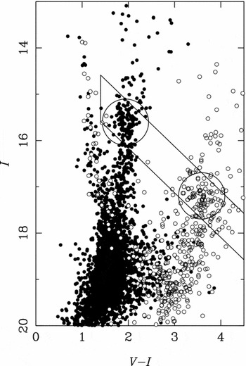
Figure 2. This is Figure 5 from Sumi (Reference Sumi2004). Shown is the colour-magnitude diagram towards two sightlines near (l, b) = ( − 0.380, −3.155), making clear the effect of interstellar extinction and reddening. The red clump shifted to a redder and fainter position.
A contending finding is that of Kunder et al. (Reference Kunder, Popowski, Cook and Chaboyer2008), who used MACHO VR measurements of RR Lyrae stars to study the reddening towards the bulge. The mean total-to-selective extinction ratio measured was $A_{\text{R}}/E(V-R) = 3.3 \pm 0.2$
, where the fit is obtained using the OLS bisector method of Feigelson & Babu (Reference Feigelson and Babu1992). In comparison, the prediction from a standard extinction curve is
$A_{\text{R}}/E(V-R) = 3.3 \pm 0.2$
, where the fit is obtained using the OLS bisector method of Feigelson & Babu (Reference Feigelson and Babu1992). In comparison, the prediction from a standard extinction curve is $A_{\text{R}}/E(V-R) = 3.34$
(Fitzpatrick Reference Fitzpatrick1999). The disagreement between the results of Kunder et al. (Reference Kunder, Popowski, Cook and Chaboyer2008), versus the results of Udalski (Reference Udalski2003), Sumi (Reference Sumi2004), and subsequent OGLE results among others is not explained at this time. It may be that the extinction curve differences are more pronounced in the range
$A_{\text{R}}/E(V-R) = 3.34$
(Fitzpatrick Reference Fitzpatrick1999). The disagreement between the results of Kunder et al. (Reference Kunder, Popowski, Cook and Chaboyer2008), versus the results of Udalski (Reference Udalski2003), Sumi (Reference Sumi2004), and subsequent OGLE results among others is not explained at this time. It may be that the extinction curve differences are more pronounced in the range $ 6\,500 \lesssim \lambda /\text{\AA} \lesssim 8\,000$
than in the range
$ 6\,500 \lesssim \lambda /\text{\AA} \lesssim 8\,000$
than in the range $ 5\,500 \lesssim \lambda /\text{\AA} \lesssim 6\,500$
. It could also be a selection effect due to the different spatial coverage. The cause of these different results has not been identified at this time.
$ 5\,500 \lesssim \lambda /\text{\AA} \lesssim 6\,500$
. It could also be a selection effect due to the different spatial coverage. The cause of these different results has not been identified at this time.
4.3. Extinction curve anomalies in the infrared
The investigations of Nishiyama et al. (Reference Nishiyama2006), Nishiyama et al. (Reference Nishiyama2008), and Nishiyama et al. (Reference Nishiyama2009) used photometry of red clump stars to conclusively demonstrate that the near-infrared extinction curve towards the inner Milky Way is non-standard. This is a more surprising result than that of extinction curve variations in the optical, as the works of Cardelli et al. (Reference Cardelli, Clayton and Mathis1989) and Fitzpatrick (Reference Fitzpatrick1999) predict a universal extinction curve in the infrared independent of variations in $R_{\text{V}}$
.
$R_{\text{V}}$
.
Nishiyama et al. (Reference Nishiyama2006) reduced photometry from the IRSF telescope towards |l| ≲ 2.0 and |b| ≲ 1.0. Nishiyama et al. (Reference Nishiyama2008) added V-band photometry from OGLE to the analysis, reporting a mean value of $A_{\text{V}}/A_{\text{Ks}} \approx 16$
, substantially higher than the standard value of ~ 9. Finally, Nishiyama et al. (Reference Nishiyama2009) added near-IR calibration from 2MASS (Skrutskie et al. Reference Skrutskie2006) and mid-infrared photometry from Spitzer/IRAC GLIMPSE survey (Benjamin et al. Reference Benjamin2003). Nishiyama et al. (Reference Nishiyama2009) measured the mean extinction coefficients
$A_{\text{V}}/A_{\text{Ks}} \approx 16$
, substantially higher than the standard value of ~ 9. Finally, Nishiyama et al. (Reference Nishiyama2009) added near-IR calibration from 2MASS (Skrutskie et al. Reference Skrutskie2006) and mid-infrared photometry from Spitzer/IRAC GLIMPSE survey (Benjamin et al. Reference Benjamin2003). Nishiyama et al. (Reference Nishiyama2009) measured the mean extinction coefficients $A_{\text{J}}:A_{\text{H}}:A_{\text{Ks}} :A_{[3.6]}:A_{[4.5]}:A_{[5.8]}:A_{[8.0]} = 3.02:1.73:1:0.50:0.39:0.36:0.43$
. The near-infrared extinction towards the Galactic bulge is well-fit by a power-law A
λ∝λ−2.0. For wavelengths longer than 2.2 μm (
$A_{\text{J}}:A_{\text{H}}:A_{\text{Ks}} :A_{[3.6]}:A_{[4.5]}:A_{[5.8]}:A_{[8.0]} = 3.02:1.73:1:0.50:0.39:0.36:0.43$
. The near-infrared extinction towards the Galactic bulge is well-fit by a power-law A
λ∝λ−2.0. For wavelengths longer than 2.2 μm ( $K_{\text{s}}$
-band), the extinction is greyer than expected from a simple extrapolation, a feature also measured by others (Indebetouw et al. Reference Indebetouw2005; Zasowski et al. Reference Zasowski2009; Gao, Jiang, & Li Reference Gao, Jiang and Li2009) and predicted by several dust models (Weingartner & Draine Reference Weingartner and Draine2001; Dwek Reference Dwek2004; Voshchinnikov et al. Reference Voshchinnikov, Il’in, Henning and Dubkova2006).
$K_{\text{s}}$
-band), the extinction is greyer than expected from a simple extrapolation, a feature also measured by others (Indebetouw et al. Reference Indebetouw2005; Zasowski et al. Reference Zasowski2009; Gao, Jiang, & Li Reference Gao, Jiang and Li2009) and predicted by several dust models (Weingartner & Draine Reference Weingartner and Draine2001; Dwek Reference Dwek2004; Voshchinnikov et al. Reference Voshchinnikov, Il’in, Henning and Dubkova2006).
Nishiyama et al. (Reference Nishiyama2009) find evidence for variations in the infrared extinction curve, but it is not significant. However, though the extinction curve is not confirmed to vary within their observational window, their results differ from other literature results towards other regions of the sky. For example, Nishiyama et al. (Reference Nishiyama2009) measure a mean value of $A_{\text{K}}/E(H-K_{\text{s}}) = 1.44 \pm 0.01$
, significantly different from the value of
$A_{\text{K}}/E(H-K_{\text{s}}) = 1.44 \pm 0.01$
, significantly different from the value of $A_{\text{K}}/E(H-K_{\text{s}}) = 1.82$
reported by Indebetouw et al. (Reference Indebetouw2005), by means of a similar methodology and data.
$A_{\text{K}}/E(H-K_{\text{s}}) = 1.82$
reported by Indebetouw et al. (Reference Indebetouw2005), by means of a similar methodology and data.
4.4. Extinction curve anomalies measured with hubble space telescope photometry
Revnivtsev et al. (Reference Revnivtsev2010) investigated the extinction curve towards a bulge window using photometry from the Hubble Space Telescope (HST) in the bandpasses F435W and F625W, which roughly correspond to Johnson-Cousins B and R, respectively. As their photometry is measured with HST, they have completely independent systematics, for example, for issues relating to photometric zero points.
They report high extinction, with an average measurement of $|A_{\text{F}625\text{W}}|=4$
, with significant variations over their total field of
$|A_{\text{F}625\text{W}}|=4$
, with significant variations over their total field of $6.6 \text{ arcmin} \times 6.6\text{ arcmin}$
. Their mean extinction coefficient is
$6.6 \text{ arcmin} \times 6.6\text{ arcmin}$
. Their mean extinction coefficient is $A_{\text{F}625\text{W}}/(A_{\text{F}435\text{W}} - A_{\text{F}625\text{W}}) = 1.25$
, corresponding to an
$A_{\text{F}625\text{W}}/(A_{\text{F}435\text{W}} - A_{\text{F}625\text{W}}) = 1.25$
, corresponding to an $R_{\text{V}} = 1.97, 2.46$
depending on whether or not one uses the parameterisations of Cardelli et al. (Reference Cardelli, Clayton and Mathis1989) or Fitzpatrick (Reference Fitzpatrick1999).
$R_{\text{V}} = 1.97, 2.46$
depending on whether or not one uses the parameterisations of Cardelli et al. (Reference Cardelli, Clayton and Mathis1989) or Fitzpatrick (Reference Fitzpatrick1999).
This can be regarded as among the most definitive demonstrations of anomalous extinction towards the bulge. On the other hand, it is a small window, and as pointed out by Nataf et al. (Reference Nataf2016), it happens to be towards a field where all indicators agree that the extinction curve is exceptionally steep.
4.5. Near-infrared reddening maps of the galactic bulge from the VVV survey
The VISTA Variables in the Via Lactea (VVV) survey (Saito et al. Reference Saito2012) yielded high-resolution, deep, near-infrared imaging over 526 deg2 of the Galactic bulge. For the first time, the photometrically discernible properties of the bulge could be discerned on a ‘global’ scale, rather than via spot duty from a few specifically targeted fields. Among the most successful data products is the global reddening map, which is to be expected given that it is a prerequisite to most other bulge science one can do with VVV.
The methodology was developed by Gonzalez et al. (Reference Gonzalez, Rejkuba, Zoccali, Valenti and Minniti2011), who measured the $(J-K_{\text{s}})$
colours of the red clump over the region 0.2 < l < 1.7, − 8 < b < −0.4. Among the first results identified by Gonzalez et al. (Reference Gonzalez, Rejkuba, Zoccali, Valenti and Minniti2011) were consistency between resulting photometric metallicity estimates and published spectroscopic results (Zoccali et al. Reference Zoccali2008; Johnson et al. Reference Johnson, Rich, Fulbright, Valenti and McWilliam2011), as well as the discernibility of the double-peaked luminosity towards high-latitude fields that is due to the peanut/X-shape of the Milky Way bulge (Nataf et al. Reference Nataf, Udalski, Gould, Fouqué and Stanek2010; McWilliam & Zoccali Reference McWilliam and Zoccali2010).
$(J-K_{\text{s}})$
colours of the red clump over the region 0.2 < l < 1.7, − 8 < b < −0.4. Among the first results identified by Gonzalez et al. (Reference Gonzalez, Rejkuba, Zoccali, Valenti and Minniti2011) were consistency between resulting photometric metallicity estimates and published spectroscopic results (Zoccali et al. Reference Zoccali2008; Johnson et al. Reference Johnson, Rich, Fulbright, Valenti and McWilliam2011), as well as the discernibility of the double-peaked luminosity towards high-latitude fields that is due to the peanut/X-shape of the Milky Way bulge (Nataf et al. Reference Nataf, Udalski, Gould, Fouqué and Stanek2010; McWilliam & Zoccali Reference McWilliam and Zoccali2010).
Gonzalez et al. (Reference Gonzalez2012) followed up with a reddening map over the coordinate range − 10.0 < l < 10.4, − 10.3 < b < 5.1, so ~ 315 deg2, broader coverage than any other bulge reddening map released either before or since. We display Figure 3 and 6 from Gonzalez et al. (Reference Gonzalez2012), as Figure 3 and 4 here. Figure 3 is a surface map of the extinction towards the bulge in $A_{\text{Ks}}$
. Values as high as
$A_{\text{Ks}}$
. Values as high as $A_{\text{Ks}} = 3.5$
are measured, corresponding to
$A_{\text{Ks}} = 3.5$
are measured, corresponding to $A_{\text{V}} \approx 50$
(Nishiyama et al. Reference Nishiyama2009; Nataf et al. Reference Nataf2016). Figure 4 is the same, but zoomed into regions of higher extinction closer to the plane to better emphasise the contrast. That kind of extinction is far too high to be measured in the optical, demonstrating the need for both infrared photometry of the inner bulge and the corresponding infrared extinction maps.
$A_{\text{V}} \approx 50$
(Nishiyama et al. Reference Nishiyama2009; Nataf et al. Reference Nataf2016). Figure 4 is the same, but zoomed into regions of higher extinction closer to the plane to better emphasise the contrast. That kind of extinction is far too high to be measured in the optical, demonstrating the need for both infrared photometry of the inner bulge and the corresponding infrared extinction maps.
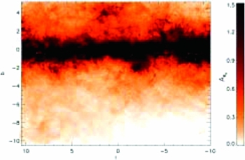
Figure 3. This is Figure 3 of Gonzalez et al. (Reference Gonzalez2012), It is the distribution of AKs
towards the Galactic bulge, as measured in VVV infrared photometry. The scale saturates for $A_{\text{Ks}} \gtrsim 1.5$
, covering the inner regions, for which the reader is referred to Figure 4 below.
$A_{\text{Ks}} \gtrsim 1.5$
, covering the inner regions, for which the reader is referred to Figure 4 below.
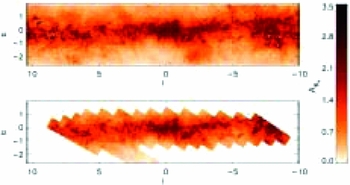
Figure 4. This is Figure 6 of Gonzalez et al. (Reference Gonzalez2012), It is the distribution of $A_{\text{Ks}}$
as in Figure 4, but zoomed in towards the inner regions to show the variation in extinction there.
$A_{\text{Ks}}$
as in Figure 4, but zoomed in towards the inner regions to show the variation in extinction there.
The analysis of Gonzalez et al. (Reference Gonzalez2012) has since been validated by Wegg & Gerhard (Reference Wegg and Gerhard2013), who report agreement at the level of ${\Delta }E(J-K_{\text{s}}) \approx 0.01$
mag. Rojas-Arriagada et al. (Reference Rojas-Arriagada2014) also validated the zero-points of the reddening map of Gonzalez et al. (Reference Gonzalez2012) by comparing photometric and spectroscopic temperatures, measuring an offset of
${\Delta }E(J-K_{\text{s}}) \approx 0.01$
mag. Rojas-Arriagada et al. (Reference Rojas-Arriagada2014) also validated the zero-points of the reddening map of Gonzalez et al. (Reference Gonzalez2012) by comparing photometric and spectroscopic temperatures, measuring an offset of ${\Delta }E(J-K_{\text{s}})=0.006 \pm 0.026$
—consistent with zero. The extinction maps of Gonzalez et al. (Reference Gonzalez2012), along with metallicity maps from Gonzalez et al. (Reference Gonzalez, Rejkuba, Zoccali, Valenti and Minniti2011), are available for download online at the BEAM calculator's webpageFootnote
3
.
${\Delta }E(J-K_{\text{s}})=0.006 \pm 0.026$
—consistent with zero. The extinction maps of Gonzalez et al. (Reference Gonzalez2012), along with metallicity maps from Gonzalez et al. (Reference Gonzalez, Rejkuba, Zoccali, Valenti and Minniti2011), are available for download online at the BEAM calculator's webpageFootnote
3
.
4.6. Optical reddening and extinction maps of the galactic bulge
The most recent, up-to-date, and broadest-in-coverage optical extinction maps of the Galactic bulge are those of Nataf et al. (Reference Nataf2013), taken with OGLE-III photometry (Udalski et al. Reference Udalski, Szymanski, Soszynski and Poleski2008). The measurements of extinction in V and I cover ≳ 90 deg2 of the bulge, nearly the entire OGLE-III survey area. As the spatial coverage was vast in both longitude and latitude, and covered a dynamical range of reddening from 0.6 ≲ E(V − I) ≲ 2.3, there was enough information to disentangle the effects of extinction curve variations and the then-unknown geometrical configuration of the Galactic bar. Further, advances in filter technology allowed a calibration of the OGLE-III filters onto the system of Landolt (Reference Landolt1992) that was very accurate, eliminating what was previously a worrisome source of uncertainty. These maps are available on the OGLE webpageFootnote 4 .
The extinction curve was confirmed to be unambiguously variable. Regression of the magnitude of the red clump versus its colour over scales as small as 30 arcmin yielded values spanning a range no smaller than $\text{d}A_{\text{I}}/\text{d}E(V-I) = 0.99 \pm 0.01$
up to
$\text{d}A_{\text{I}}/\text{d}E(V-I) = 0.99 \pm 0.01$
up to $\text{d}A_{\text{I}}/\text{d}E(V-I) = 1.46 \pm 0.03$
(see Figure 7 of Nataf et al. Reference Nataf2013). These variations can be found even at the same level of reddening, so they are not due to the convolution of the photometric bandpass with the extinction curve, or other non-linear effects.
$\text{d}A_{\text{I}}/\text{d}E(V-I) = 1.46 \pm 0.03$
(see Figure 7 of Nataf et al. Reference Nataf2013). These variations can be found even at the same level of reddening, so they are not due to the convolution of the photometric bandpass with the extinction curve, or other non-linear effects.
Demonstrating that the extinction curve is variable is not the same as solving for its variations. It was shown that the extinction curve could vary on scales smaller than 30 $\text{arcmin}$
, and thus the method of measuring regressions of extinction versus reddening towards relatively small regions was now demonstrated to be insufficient. Nataf et al. (Reference Nataf2013) discuss several failed attempts to constrain the total-to-selective extinction ratio as a function of sightline and why they did not work.
$\text{arcmin}$
, and thus the method of measuring regressions of extinction versus reddening towards relatively small regions was now demonstrated to be insufficient. Nataf et al. (Reference Nataf2013) discuss several failed attempts to constrain the total-to-selective extinction ratio as a function of sightline and why they did not work.
What ultimately solved the issue was the combination of the E(V − I) reddening maps from Nataf et al. (Reference Nataf2013) with the $E(J-K_{\text{s}})$
reddening maps from Gonzalez et al. (Reference Gonzalez2012), where the ratio is shown in Figure 5, which is Figure 12 of Nataf et al. (Reference Nataf2013). The ratio of the two could be measured over scales as small as 3
$E(J-K_{\text{s}})$
reddening maps from Gonzalez et al. (Reference Gonzalez2012), where the ratio is shown in Figure 5, which is Figure 12 of Nataf et al. (Reference Nataf2013). The ratio of the two could be measured over scales as small as 3 $\text{arcmin}$
, a correlation between
$\text{arcmin}$
, a correlation between $E(J-K_{\text{s}})/E(V-I)$
and
$E(J-K_{\text{s}})/E(V-I)$
and $A_{\text{I}}/E(V-I)$
was measured and used to report the extinction everywhere. The best fit was found to be
$A_{\text{I}}/E(V-I)$
was measured and used to report the extinction everywhere. The best fit was found to be
 $$\begin{eqnarray}
A_{\text{I}} &=& 0.7465 \times E(V - I) + 1.3700 \times E(J - K_{\text{s}}) \nonumber\\
& = &1.217\times E(V - I ) \\
&&\times\, (1 + 1.126 \times (E(J - K_{\text{s}} )/E(V - I ) - 0.3433)).\nonumber
\end{eqnarray}$$
$$\begin{eqnarray}
A_{\text{I}} &=& 0.7465 \times E(V - I) + 1.3700 \times E(J - K_{\text{s}}) \nonumber\\
& = &1.217\times E(V - I ) \\
&&\times\, (1 + 1.126 \times (E(J - K_{\text{s}} )/E(V - I ) - 0.3433)).\nonumber
\end{eqnarray}$$
Assuming that $A_{\text{I}}/E(V-I)$
correlates with
$A_{\text{I}}/E(V-I)$
correlates with $E(J-K_{\text{s}})/\break E(V-I)$
is equivalent to assuming a single, dominant parameter to extinction curve variations (e.g.
$E(J-K_{\text{s}})/\break E(V-I)$
is equivalent to assuming a single, dominant parameter to extinction curve variations (e.g. $R_{\text{V}}$
). The precision in
$R_{\text{V}}$
). The precision in $A_{\text{I}}$
is estimated as ~ 0.04 mag, and thus better than 4%. This two-colour extinction correction was confirmed as being more reliable than any dereddening method based on (V − I) colour alone in the analysis of bulge RR Lyrae stars by (Pietrukowicz et al. Reference Pietrukowicz2015). It was shown that Equation (7) gives a more reasonable and a substantially tighter distance distribution function to bulge RR Lyrae stars, and has thus been adopted by other RR Lyrae bulge studies (Kunder et al. Reference Kunder2015).
$A_{\text{I}}$
is estimated as ~ 0.04 mag, and thus better than 4%. This two-colour extinction correction was confirmed as being more reliable than any dereddening method based on (V − I) colour alone in the analysis of bulge RR Lyrae stars by (Pietrukowicz et al. Reference Pietrukowicz2015). It was shown that Equation (7) gives a more reasonable and a substantially tighter distance distribution function to bulge RR Lyrae stars, and has thus been adopted by other RR Lyrae bulge studies (Kunder et al. Reference Kunder2015).
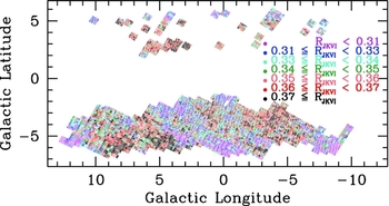
Figure 5. This is Figure 12 of Nataf et al. (Reference Nataf2013). Shown is the ratio of $E(J-K_{\text{s}}$
measured by Gonzalez et al. (Reference Gonzalez2012) to E(V − I) measured from OGLE photometry. The data is shown in equal area septiles. The extinction curve is clearly variable, spanning the range
$E(J-K_{\text{s}}$
measured by Gonzalez et al. (Reference Gonzalez2012) to E(V − I) measured from OGLE photometry. The data is shown in equal area septiles. The extinction curve is clearly variable, spanning the range $0.31 \rightarrow E(J-K_{\text{s}})/E(V-I) \rightarrow 0.17$
between the 14th and 86th percentiles.
$0.31 \rightarrow E(J-K_{\text{s}})/E(V-I) \rightarrow 0.17$
between the 14th and 86th percentiles.
The issue of extinction curve variations towards the bulge was followed up by Nataf et al. (Reference Nataf2016), who added measurements of E(I − J) to increase the diagnostic power—three colours were measured rather than two. A comparison of two independent extinction curve ratios is shown in Figure 6. What Nataf et al. (Reference Nataf2016) demonstrated, above and beyond the previous findings of variable extinction, is that the extinction curve towards many bulge sightlines cannot be matched by the predictions of Cardelli et al. (Reference Cardelli, Clayton and Mathis1989) and Fitzpatrick (Reference Fitzpatrick1999) regardless of how $R_{\text{V}}$
is varied, demonstrating a total failure of those empirical frameworks towards the inner Milky Way. That is shown in Figure 6, where not only does the prediction of Fitzpatrick (Reference Fitzpatrick1999) for
$R_{\text{V}}$
is varied, demonstrating a total failure of those empirical frameworks towards the inner Milky Way. That is shown in Figure 6, where not only does the prediction of Fitzpatrick (Reference Fitzpatrick1999) for $R_{\text{V}}=3.1$
(the green circle) fail to intersect the measurements, but rather the green line (variations in
$R_{\text{V}}=3.1$
(the green circle) fail to intersect the measurements, but rather the green line (variations in $R_{\text{V}}$
) never intersects the measurements. Further, as can also be seen in Figure 6, the variations in the extinction curve are not necessarily correlated between different extinction curve ratios. Both
$R_{\text{V}}$
) never intersects the measurements. Further, as can also be seen in Figure 6, the variations in the extinction curve are not necessarily correlated between different extinction curve ratios. Both $A_{\text{I}}/E(V-I)$
and
$A_{\text{I}}/E(V-I)$
and $E(J-K_{\text{s}})/E(I-J)$
vary significantly, but they do so independently. This necessitates additional degrees of freedom beyond
$E(J-K_{\text{s}})/E(I-J)$
vary significantly, but they do so independently. This necessitates additional degrees of freedom beyond $R_{\text{V}}$
.
$R_{\text{V}}$
.
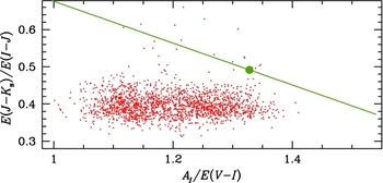
Figure 6. This is Figure 8 of Nataf et al. (Reference Nataf2016). The distribution of two extinction curve ratios, $E(J-K_{\text{s}})/E(I-J)$
and
$E(J-K_{\text{s}})/E(I-J)$
and $A_{\text{I}}/E(V-I)$
is shown as the red points, with the prediction of Fitzpatrick (Reference Fitzpatrick1999) shown in green with the green circle denoting the
$A_{\text{I}}/E(V-I)$
is shown as the red points, with the prediction of Fitzpatrick (Reference Fitzpatrick1999) shown in green with the green circle denoting the $R_{\text{V}}=3.1$
case. The predictions are poor match to the data regardless of the value of
$R_{\text{V}}=3.1$
case. The predictions are poor match to the data regardless of the value of $R_{\text{V}}$
.
$R_{\text{V}}$
.
Nataf et al. (Reference Nataf2016) then took the issue a step further and argued that interstellar extinction curve variations towards the bulge, which are at very high signal-to-noise and offer a large sample size due to the high reddening and high surface density of standard crayons, might be used as an essential laboratory for cosmology. The first motivation mentioned was the challenge of inferring dust properties towards Type Ia SNe. The mean extinction curve towards Type Ia SNe is $R_{\text{V}} \approx 2.05$
(Rubin et al. Reference Rubin2015). The uncertainties in the treatment of extinction have been evaluated as the second largest source of systematic error in the determination of the dark energy equation-of-state parameter ‘w’ (Scolnic et al. Reference Scolnic2014). This estimate assumes that the uncertainty is an uncertainty in
$R_{\text{V}} \approx 2.05$
(Rubin et al. Reference Rubin2015). The uncertainties in the treatment of extinction have been evaluated as the second largest source of systematic error in the determination of the dark energy equation-of-state parameter ‘w’ (Scolnic et al. Reference Scolnic2014). This estimate assumes that the uncertainty is an uncertainty in $R_{\text{V}}$
, and does not include the fact that for some sightlines the extinction curve is not fit by any value of
$R_{\text{V}}$
, and does not include the fact that for some sightlines the extinction curve is not fit by any value of $R_{\text{V}}$
, which is now demonstrated as a fact of nature.
$R_{\text{V}}$
, which is now demonstrated as a fact of nature.
5 EXTINCTION TOWARDS GALACTIC BULGE GLOBULAR CLUSTERS
The list of E(B − V) values towards bulge globular clusters to be found in the catalogue of Harris (Reference Harris1996, 2010 edition) would be difficult to make suitable in the context of this review. The literature sources are heterogeneous in methodology, accuracy, and precision. Further, the number reported in the catalogue, E(B − V) is rarely or never the number actually measured by any of these methods for the heavily reddened bulge globular clusters. Rather, some other reddening index is measured, and then converted to E(B − V) using reddening coefficients that are now demonstrated to be of dubious merit.
One exception is the compilation of Recio-Blanco et al. (Reference Recio-Blanco2005), which was derived from the HST treasury program of Piotto et al. (Reference Piotto2002). Reddening determinations are made in the system of the observations, E(F439W − F555W), by measuring the colour excess of the horizontal branch. In Table 2, we list the measurements of Recio-Blanco et al. (Reference Recio-Blanco2005), along with those of Gonzalez et al. (Reference Gonzalez2012) towards the same sightlines, using a 6 arcmin window input into the BEAM calculator. From Table 11 and 12 of Holtzman et al. (Reference Holtzman1995), we know that E(F439W − F555W) ≈ E(B − V), not surprising as these are nearly identical filter pairs.
Table 2. Compilation of reddening measurements towards bulge globulars from Recio-Blanco et al. (Reference Recio-Blanco2005) and towards the same sightlines by Gonzalez et al. (Reference Gonzalez2012).
The globular cluster NGC 6544 is an outlier, with $E(F439W-F555W)/E(J-K_{\text{s}})=1.07$
. This is likely due to the globular cluster being relatively closeby, ~ 3 kpc from the Sun (Harris Reference Harris1996, 2010 edition), and thus only ~ 120 pc below the Galactic plane and likely in front of a lot of the dust. For the remaining globular clusters, I measure
$E(F439W-F555W)/E(J-K_{\text{s}})=1.07$
. This is likely due to the globular cluster being relatively closeby, ~ 3 kpc from the Sun (Harris Reference Harris1996, 2010 edition), and thus only ~ 120 pc below the Galactic plane and likely in front of a lot of the dust. For the remaining globular clusters, I measure $E(J-K_{\text{s}})/E(F439W-F555W)=0.41$
. The prediction from Cardelli et al. (Reference Cardelli, Clayton and Mathis1989) is
$E(J-K_{\text{s}})/E(F439W-F555W)=0.41$
. The prediction from Cardelli et al. (Reference Cardelli, Clayton and Mathis1989) is $E(J-K_{\text{s}})/E(F439W-F555W) \approx 0.53$
.
$E(J-K_{\text{s}})/E(F439W-F555W) \approx 0.53$
.
The high reddening towards bulge globular clusters has meant that they tend to be less studied than most other globular clusters, due to the greater difficulty of obtaining deep photometry. However, this is beginning to change, as these clusters are interesting in their own right. It is plausible that in the near future globular clusters may reprise their historical role as leading diagnostics of the extinction towards the bulge, given their potential for high-resolution, multi-wavelength extinction maps. For example, Massari et al. (Reference Massari2012) measure differential reddening exceeding ${\delta}E(J-K_{\text{s}}) = 0.30$
over scales as small as 2 arcsec towards Terzan 5 (Massari et al. Reference Massari2012). Interested readers are referred to the review of bulge globular clusters found elsewhere in this special issue, Bica, Ortolani, & Barbuy (Reference Bica, Ortolani and Barbuy2015), for further information on systems.
${\delta}E(J-K_{\text{s}}) = 0.30$
over scales as small as 2 arcsec towards Terzan 5 (Massari et al. Reference Massari2012). Interested readers are referred to the review of bulge globular clusters found elsewhere in this special issue, Bica, Ortolani, & Barbuy (Reference Bica, Ortolani and Barbuy2015), for further information on systems.
6 DISCUSSION AND CONCLUSION
The magnitude of progress in recent decades in the study of extinction towards the Galactic bulge is clearly high. The community has gone from its first extinction map covering an area of 40 $\text{arcmin}\times$
40
$\text{arcmin}\times$
40 $\text{arcmin}$
near Baade's window (Stanek Reference Stanek1996), to reddening maps spanning nearly the entirety of the bulge (Gonzalez et al. Reference Gonzalez2012). It has shifted from assuming literature values of the interstellar extinction coefficients, to actively measuring them and in fact finding a ~ 20–25% offset (Nishiyama et al. Reference Nishiyama2009; Nataf et al. Reference Nataf2016).
$\text{arcmin}$
near Baade's window (Stanek Reference Stanek1996), to reddening maps spanning nearly the entirety of the bulge (Gonzalez et al. Reference Gonzalez2012). It has shifted from assuming literature values of the interstellar extinction coefficients, to actively measuring them and in fact finding a ~ 20–25% offset (Nishiyama et al. Reference Nishiyama2009; Nataf et al. Reference Nataf2016).
In spite of this progress, there remains a need for further progress, as the advances in this field are mirrored by advances in other areas of astronomy which necessitates superior accuracy and precision. Three areas in need of improvement are those of differential reddening estimates, understanding of the ‘anomalous’ extinction coefficients, and an integrated study of the planetary nebulae.
Though the extinction maps of Gonzalez et al. (Reference Gonzalez2012) yield precise and accurate estimates of $E(J-K_{\text{s}})$
nearly everywhere towards the bulge, it's the case that differential reddening can exceed ~ 10% of the mean reddening towards bulge observing windows as small as 3
$E(J-K_{\text{s}})$
nearly everywhere towards the bulge, it's the case that differential reddening can exceed ~ 10% of the mean reddening towards bulge observing windows as small as 3 $\text{arcmin}$
(Nataf et al. Reference Nataf2013). This was estimated by measuring that the width of the red giant branch in colour space correlates with the mean reddening, which cannot be due to intrinsic factors as the gradient in metallicity dispersion of the bulge is null or shallow (Zoccali et al. Reference Zoccali2008). Massari et al. (Reference Massari2012) measured differential extinction towards the globular cluster Terzan 5 exceeding ~ 25%, over a small field of
$\text{arcmin}$
(Nataf et al. Reference Nataf2013). This was estimated by measuring that the width of the red giant branch in colour space correlates with the mean reddening, which cannot be due to intrinsic factors as the gradient in metallicity dispersion of the bulge is null or shallow (Zoccali et al. Reference Zoccali2008). Massari et al. (Reference Massari2012) measured differential extinction towards the globular cluster Terzan 5 exceeding ~ 25%, over a small field of $ 200 \text{arcsec} \times 200 \text{arcsec}$
. Some progress will be needed on this effect as Galactic astronomy transitions to being a precision science, there may be hope by combining additional photometry from new surveys like the Blanco DECam Bulge Survey (Clarkson et al. Reference Clarkson2014).
$ 200 \text{arcsec} \times 200 \text{arcsec}$
. Some progress will be needed on this effect as Galactic astronomy transitions to being a precision science, there may be hope by combining additional photometry from new surveys like the Blanco DECam Bulge Survey (Clarkson et al. Reference Clarkson2014).
The issue of different extinction coefficients towards the bulge is also a strange one. I am aware of no theoretical prediction within the literature that would explain why this is so. Minniti et al. (Reference Minniti2014) conjectures a ‘Great Dark Lane’ between the Sun and the bulge, this could be the explanation, but at this time there have been no follow-up publications, and thus no estimates of the extinction curve specific to the Great Dark Lane. It was conceivable that the anomalous extinction could just be an artifact of incorrect assumptions as to what the ‘standard’ extinction curve is, but this conjecture has become less and less plausible. Udalski (Reference Udalski2003) showed that the reddening towards the bulge is systematically different to that towards the Large Magellanic Cloud in a manner independent of systematics, by means of a purely differential analysis. Nataf et al. (Reference Nataf2016) combined four measures of extinction in the bandpasses $VIJK_{\text{s}}$
to show no compatibility between bulge extinction coefficients and literature extinction coefficients even after allowing for the range of ‘standard’ extinction curves to be found in the literature. Schlafly et al. (Reference Schlafly, Meisner and Stutz2016) have recently confirmed that literature values of the ‘standard’ extinction curve are in fact not correct descriptions of nature even in the solar neighbourhood. The discrepancy remains regardless, their Table 5 shows that their measured mean extinction coefficients for the local interstellar medium remain distinct from the measured values towards the bulge, with an offset of ~ 16% for
$VIJK_{\text{s}}$
to show no compatibility between bulge extinction coefficients and literature extinction coefficients even after allowing for the range of ‘standard’ extinction curves to be found in the literature. Schlafly et al. (Reference Schlafly, Meisner and Stutz2016) have recently confirmed that literature values of the ‘standard’ extinction curve are in fact not correct descriptions of nature even in the solar neighbourhood. The discrepancy remains regardless, their Table 5 shows that their measured mean extinction coefficients for the local interstellar medium remain distinct from the measured values towards the bulge, with an offset of ~ 16% for $E(V-I)/E(J-K_{\text{s}})$
.
$E(V-I)/E(J-K_{\text{s}})$
.
The planetary nebulae measurements are their own diagnostic, with completely independent systematics. Are the offsets in the Balmer decrement measured by Stasińska et al. (Reference Stasińska, Tylenda, Acker and Stenholm1992) and Ruffle et al. (Reference Ruffle2004) towards bulge planetary nebulae really due to additional opacity in the radio continuum, as argued by Pottasch & Bernard-Salas (Reference Pottasch and Bernard-Salas2013)? If the extinction coefficients are non-standard, are we measuring the same phenomenon as measured with red clump and RR Lyrae stars? If they are in fact standard, how can that be reconciled with the measurement of extinction anomalies towards red clump and RR Lyrae stars? There is manifest potential for elucidation here, should there be an integrated study in the future.
ACKNOWLEDGEMENTS
DMN was supported by the Australian Research Council grant FL110100012. I thank Albert Zijlstra for helpful discussions. I thank the anonymous referee for a constructive and detailed report.


