


1 INTRODUCTION
The central parts of our Galaxy were prospected by Baade (Reference Baade1946), in order to detect its nucleus, and to have an indication of the morphological type of our Galaxy. The so-called Baade's Window was revealed, and from variable stars identified in the field, the bulge stellar population was identified to be similar to that defined in Baade (Reference Baade1944) as population II. In the early 60s, the notion of a Galactic bulge was already established (e.g. Courtes & Cruvellier Reference Courtes and Cruvellier1960). McClure (Reference McClure1969) found that the bulge stars were super metal-rich compared to the stars nearby the Sun. Whitford and Rich (Reference Whitford and Rich1983) confirmed the high metal content of bulge stars from individual star spectroscopy.
Catalogues prepared along the decades show a steady growth of overall samples of globular clusters (hereafter referred to as GCs), together with photometric and spectroscopic information. Cannon (Reference Cannon1929) used the Harvard plate spectra to give integrated spectral types of 45 GCs. Mayall (Reference Mayall1946) measured radial velocities of 50 GCs, and the integrated spectral types of 40 of them. Kinman (Reference Kinman1959) listed 32 GCs with indication of metallicity from their integrated spectra; Morgan (Reference Morgan1959) directed efforts on a relatively bright sample of 13 bulge GCs, now known to be metal-rich.
Surveys with Schmidt plates since the 60s provided the Palomar and ESO star clusters, among others. Terzan (Reference Terzan1968 and references therein) significantly increased the number of central GCs by reporting new faint ones in the bulge direction. These discoveries provided an important sample of GCs in the bulge.
Other studies of GC overall samples were presented by van den Bergh (Reference van den Bergh1967), Zinn (Reference Zinn1985 and references therein), Bica & Pastoriza (Reference Bica and Pastoriza1983). Webbink (Reference Webbink1985) provided a catalogue of 154 GCs and candidates, with an important impact on subsequent observational efforts. More recently, Harris (Reference Harris1996, updated in 2010, hereafter Harris10)Footnote 1 reports properties for 157 GCs.
It is interesting to see how the notion of GCs pertaining to the bulge and their spatial distribution evolved in the last decades. Frenk & White (Reference Frenk and White1982) found evidence that metal-rich GCs formed a bar-like structure. Based on metallicity, scale height, and rotational velocities available at that time, Armandroff (Reference Armandroff1989 and references therein) interpreted a sample of low Galactic latitude metal-rich GCs as belonging to a disk system. Minniti (Reference Minniti1995) instead, from metallicity and kinematics of GCs in the central 3 kpc (about 20°) from the Galactic centre, found evidence for these GCs to belong to the bulge. Côté (Reference Côté1999) derived metallicities and radial velocities from high-resolution spectroscopy for a significant sample of GCs within 4 kpc from the Galactic centre. He concluded that metal-rich GCs are associated with the bulge/bar rather than the thick disk.
An important step in the understanding of the nature of the bulge GCs was presented by Ortolani et al. (Reference Ortolani1995), where the metal-rich GCs NGC 6528 and NGC 6553 were found to have an old age, identical to the bulk of the bulge field stars and comparable to that of the halo clusters. Barbuy et al. (Reference Barbuy, Bica and Ortolani1998) derived new results and summarised the properties of 17 GCs in the bulge projected within 5° of the Galactic centre. They concluded that these clusters shared comparable properties with the bulge field stars, including not only metal-rich GCs but also intermediate metallicity ones. They also found that there are no clusters in a strip 2.8° wide centred at about 0.5° south of the Galactic plane.
Several comprehensive recent reviews have addressed the stellar populations, both field and GCs, in the Galactic bulge (e.g. Harris Reference Harris, Labhardt and Binggeli2001; Rich Reference Rich, Oswal and Gilmore2013; Gonzalez & Gadotti Reference Gonzalez, Gadotti, Laurikainen, Peletier and Gadotti2016). These reviews address also comparisons of the Galactic bulge with external galaxies.
In the following, we describe recent advances on detailed chemical abundances, distances, kinematical properties, and hints on possible association with subsystems in the central region of the Galaxy. We also prepare for the future by defining a bulge GC sample, which includes suggestions for future studies, in terms of unstudied objects. In particular, it is clear that proper motion derivation is still needed for most GCs.
2 THE SAMPLE OF BULGE GLOBULAR CLUSTERS
In the past, angular distances from the Galactic centre were the basis for selecting bulge GCs in the central parts of the Galaxy (e.g. Zinn Reference Zinn1985; Barbuy et al. Reference Barbuy, Bica and Ortolani1998).
As a first approach, we selected clusters with angular distances below 20°. Our next step was to use the Galactocentric distances of the clusters, given that now they are more reliable—see Harris10. We adopted a distance to the Galactic centre of 8 kpc (Bobylev et al. Reference Bobylev, Mosenkov, Bajkova and Gontcharov2014; Reid et al. Reference Reid2014). For selecting the clusters, we have experimented different distances from the Galactic centre of 6, 5, 4, and 3 kpc. In each case, we checked for bulge clusters and halo intruders. We concluded that a cut-off of 3 kpc is best in terms of isolating a bona-fide bulge cluster sample, with little contamination. We finally applied a metallicity filter: Zoccali et al. (2008), Hill et al. (Reference Hill2011), Ness et al. (Reference Ness, Freeman and Athanassoula2013a), and Rojas-Arriagada et al. (Reference Rojas-Arriagada2014) have shown that the lower metallicity end of the bulge is around [Fe/H] = − 1.3. This is confirmed with the findings by Walker and Terndrup (1991), Lee (Reference Lee1992), Dékány et al. (Reference Dékány2013), Pietrukowicz et al. (Reference Pietrukowicz2012, Reference Pietrukowicz2015), and Gran et al. (Reference Gran2016), Dékány et al. (Reference Dékány2013) and Lee (Reference Lee1992), all of them having demonstrated that there is a peak of RR Lyrae with [Fe/H] ≈ − 1.0, centrally concentrated and spheroidal (except for Pietrukowicz et al. Reference Pietrukowicz2015 that found it to be elongated), corresponding to an old bulge. We verified that GCs with [Fe/H] < − 1.5 corresponded to well-known halo clusters in most cases, and we excluded GCs with [Fe/H]< –1.5.
Criteria using the space velocity V, as proposed by Dinescu, Girard, & van Altena (Reference Dinescu, Girard and van Altena1997), Dinescu, van Altena, & Girard (Reference Dinescu, van Altena and Girard1999a), Dinescu, Girard, & van Altena (Reference Dinescu, Girard and van Altena1999b), Dinescu et al. (Reference Dinescu, Girard, van Altena and López2003), and Casetti-Dinescu et al. (Reference Casetti-Dinescu2007, Reference Casetti-Dinescu2010, Reference Casetti-Dinescu2013), are only feasible if proper motions are available, besides radial velocities. In particular, Dinescu et al. (Reference Dinescu, Girard, van Altena and López2003) verified the classification of clusters as members of different galaxy components in terms of kinematics. The use of this criterion is possible for about a third of the GCs, at the present stage. Gaia results in a few years will bring higher precision, and new data for a number of GCs. A few groups are applying proper motion cleaning to bulge clusters (e.g. Dinescu et al. Reference Dinescu, Girard, van Altena and López2003; Rossi et al. Reference Rossi2015). Therefore, Carretta et al. (Reference Carretta2010) criterion of space velocity V values to select stellar populations, is not possible presently for having only the radial velocity in many cases, but may be applicable in a few years.
In Table 1, we present the selected bulge clusters, following the criteria explained above. Djorgovski 1 is added to the list, because it was in the Barbuy et al. (Reference Barbuy, Bica and Ortolani1998)'s list, and the distance available in Harris10, based on infrared data, is probably overestimated. The clusters are ordered by right ascension, to be compatible with Harris10.
Table 1. Bulge globular clusters. Reddening values in columns 4, 5, and 6 correspond to Harris10, Valenti et al. (Reference Valenti, Ferraro and Origlia2007), and our studies along the years. Galactocentric distances and metallicities are from Harris10, except for UKS 1 (see Section 3). References: 1: Casetti-Dinescu et al. Reference Casetti-Dinescu2010; 2: Ortolani et al. Reference Ortolani2011; 3: Rossi et al. Reference Rossi2015; 4: Casetti-Dinescu et al. Reference Casetti-Dinescu2013; 5: Dinescu et al. Reference Dinescu, Girard, van Altena and López2003; 6: Zoccali et al. Reference Zoccali2001; 7: Cudworth & Hanson Reference Cudworth and Hanson1993. Notes: *sample from Barbuy et al. Reference Barbuy, Bica and Ortolani1998.

The distances from the Sun are from Harris10 mainly based on the visual magnitude of the HB, while Valenti, Ferraro, & Origlia (Reference Valenti, Ferraro and Origlia2007) give distances based on isochrone fitting in JHK. We also report distances derived from the Galactic centre, as given by Harris10. For Kronberger 49, not listed in Harris10, data are from Ortolani et al. (Reference Ortolani2012). The distance derivation is crucial in order to get the position of the clusters relative to the Galactic centre and the bar. In most cases, for a cluster located inside the bar, its orbit is trapped, given the high mass of the bar. In fact, more than half the bulge mass is in the bar, and for this reason, the bulge clusters that show low kinematics are probably trapped (Rossi et al. Reference Rossi2015). Given the old age of the clusters, it is likely that they were formed before the bar, and later trapped. The dynamical behaviour of such clusters was illustrated for HP 1 (Ortolani et al. Reference Ortolani2011), and for nine GCs by Rossi, Ortolani, Casotto, Barbuy, and Bica (in preparation), all of them showing a low maximum height.
2.1. Intruders and missed bulge clusters?
In Table 2, we list possible intruders to our main selection, as well as limiting cases, and we collected a few more GCs with other distance and metallicity criteria. Subsamples are classified as follows:
-
(a) Probable halo intruders with [Fe/H] < −1.5: we found 6 GCs with distances to the Galactic centre smaller than 3 kpc (our selected bulge volume), but with metallicity lower than [Fe/H] < −1.5, and besides with very high spatial velocities (Dinescu et al. Reference Dinescu, van Altena and Girard1999a; Casetti-Dinescu et al. Reference Casetti-Dinescu2010), all pointing to perigalactic locations of halo GCs.
-
(b) Outer bulge shell with distances 3 < R < 4.5 kpc: this surrounding bulge shell does probably contain true bulge GCs, that should be near apogalacticon. Interestingly, the few space velocities available (Dinescu et al. Reference Dinescu, van Altena and Girard1999a, Cudworth & Hanson Reference Cudworth and Hanson1993) for this sample are rather low.
-
(c) Outer bulge shell intruders: five GCs are located in this shell (b), but showing low metallicities, as for example M22, having also a high velocity typical of halo, like in group (a).
-
(d) Metal-rich GCs ([Fe/H] > −1.0) beyond R > 4.5 kpc: this sample corresponds to the ones that conveyed the idea of ‘disk GCs’ (e.g. Armandroff Reference Armandroff1989). Many of these key and well-known GCs do not have space velocities derived so far. This would be of great interest to constrain the possibility to link them to the thick disk.
-
(e) Intruders to (d). Data for FSR 1767 are from Bonatto et al. (Reference Bonatto, Bica, Ortolani and Barbuy2007, Reference Bonatto, Bica, Ortolani and Barbuy2009).
-
(f) Little studied GCs without enough parameters: probably key objects for future analysis (Section 6). In Figure 1 are plotted distances (kpc) vs. metallicity [Fe/H], space velocity VS (km s−1) vs. [Fe/H] and vs. distance (kpc), for the bulge sample (Table 1) and intruders (Table 2), for which such data are available.
Table 2. Intruders and missed bulge clusters? (a) Possible halo intruders with [Fe/H] < −1.5; (b) Shell: Distances 3 < R < 4.5 kpc; (c) Intruders to shell; (d) [Fe/H] > −1.0 and R > 4.5 kpc; (e) Intruders to disc; (f) no parameters enough; *looks halo intruder in the shell, despite distance; **see Section 3. References: 1: Casetti-Dinescu et al. Reference Casetti-Dinescu2010; 4: Casetti-Dinescu et al. Reference Casetti-Dinescu2013; 7: Cudworth and Hanson Reference Cudworth and Hanson1993; 8: Dinescu et al. Reference Dinescu, Girard and van Altena1997; 9: Casetti-Dinescu et al. Reference Casetti-Dinescu2007; 10: Casetti-Dinescu et al. Reference Casetti-Dinescu2013.


2.2. Multiple population clusters in the bulge
Terzan 5 was identified to have at least two stellar populations and given its high mass, it was proposed to be a stripped dwarf galaxy (Ferraro et al. Reference Ferraro2009; Origlia et al. Reference Origlia2013; Massari et al. Reference Massari2014). Saracino et al. (Reference Saracino2015) concluded that Liller 1 is as massive as Terzan 5 or ω Centauri. These massive clusters have absolute magnitudes around M V ≈ −10.
On the other hand, the faintest bulge GCs are as faint as M V ≈ −4, such as Terzan 9 and AL 3. These magnitudes are comparable to those of the ultra-faint galaxies (e.g. McConnachie Reference McConnachie2012; Bechtol et al. Reference Bechtol2015).
By multiple stellar populations, we refer to different metallicities [Fe/H] and/or age in a same cluster. For most clusters, there are hints of two populations, but no difference in metallicity. A comprehensive discussion on Na-O anticorrelation was given by Gratton et al. (Reference Gratton2015), where differences between red and blue horizontal branch (HB) stars allow to derive some important conclusions. See further discussions on multiple populations revealed by Na-O anticorrelations in Section 4. Since this effect appears to be present for most clusters, this is incorporated in the definition of GCs, and it is not a concern in the present work.
3 DISTANCES
Distances of bulge GCs are mainly based on the HB luminosity level. The calculation of distances depends on three basic inputs: (1) the HB absolute magnitude, (2) the reddening, and (3) the reddening law. These three datasets slightly depend on the metallicity. The HB absolute magnitude may also depend on the He abundance. The current statistics is based mostly on the distances reported in Harris10, where the HB level is given by the relation: M(HB) = 0.16[Fe/H] + 0.84. In Harris10, if the HB level is not available, specific references are used. This relation is somewhat different from that used by Barbuy et al. (Reference Barbuy, Bica and Ortolani1998) in their catalogue of 17 inner bulge clusters, adopted from Jones et al. (Reference Jones, Carney, Storm and Latham1992): M(HB) = 0.16[Fe/H] + 0.98. This latter relation gives an HB level of about 0.14 mag fainter, producing as well smaller distance moduli, but this difference is negligible when compared to other uncertainties. It is also important to point out that the main difference between Harris10 and Barbuy et al. (Reference Barbuy, Bica and Ortolani1998) values, is that the latter was based on optical colour–magnitude diagrams (CMDs) only. The list of distances also makes use of the JHK CMDs when it is considered more reliable. Finally, the catalogue by Bica et al. (Reference Bica, Bonatto, Barbuy and Ortolani2006) uses basically the same assumptions as Harris10.
Reddening and reddening law: The reddening is a key parameter in the derivation of the distances based on the photometric technique. For most of the low latitude bulge GCs, an error of 5% in reddening produces a typical error of ~ 15% in the absorption, which propagates with the same fraction to the distance modulus. In Harris10, the reddening has been derived from Webbink (Reference Webbink1985), Zinn (Reference Zinn1985), and Reid et al. (1988). The standard reddening law (R V = 3.1) has been used to derive the visual absorption. Bica et al. (Reference Bica, Bonatto, Barbuy and Ortolani2006) used basically the same input values, but they converted E(B − V) into A V using R V = 3.1 for clusters with [Fe/H] < − 1.0 and R V = 3.6 for [Fe/H] > −1.0 following Grebel and Roberts (Reference Grebel and Roberts1995), and R V values have been interpolated in the intermediate metallicity interval. In principle, this choice should produce shorter distances than Harris10 for high metallicity clusters. A different computation was performed for most of the inner bulge clusters presented in Barbuy et al. (Reference Barbuy, Bica and Ortolani1998). Equation (A1) of Dean, Warpen, & Cousins (Reference Dean, Warren and Cousins1978) was used to convert E(V − I) to E(B − V) and then the reddening dependence of R V on E(B − V) as given in Olson (Reference Olson1975) has been used to convert E(B − V) into A V: R V = 3.1 + 0.05([Fe/H]).
Independent distances and reddening values have been obtained by Valenti et al. (Reference Valenti, Ferraro and Origlia2007) for 37 bulge clusters, using infrared JHK photometry. The main advantage of the JHK derived distances is that the reddening versus absorption ratio is almost constant even if R V varies (Fitzpatrick Reference Fitzpatrick1999; Cardelli, Clayton, & Mathis Reference Cardelli, Clayton and Mathis1989). The comparison of the optical versus IR distances give a chance to probe the reddening law, in the optical regime, in the direction of the Galactic bulge.
Figure 2 shows the distance differences between different R V values versus reddening. The absolute magnitude of the horizontal branch M(HB) is assumed to be of M(HB) = 0.68 for [Fe/H] = − 1.0, at E(B − V)=0. Therefore, at the distance of the Galactic centre, assumed here to be of 8 kpc, the distance modulus is m − M = 14.5, and m(HB) = 14.5 + 0.68 = 15.18. So for the zero point, we assume: E(B − V) = 0, m(HB) = 15.18. We use 12 clusters in common with Valenti et al. (Reference Valenti, Ferraro and Origlia2007), and adding Terzan 9 (Ortolani, Bica, & Barbuy Reference Ortolani, Bica and Barbuy1999). From this sample, an average distance difference of d(IR)–d(optical) = 0.65 kpc has been derived. In the infrared sample, we have also three clusters (Terzan 4, Terzan 5, and NGC 6528) with data from Hubble Space Telescope (HST)/NICMOS (Ortolani et al. Reference Ortolani, Barbuy, Bica, Zoccali and Renzini2007). In these cases, we adopted an average value between NICMOS and Valenti et al. (Reference Valenti, Ferraro and Origlia2007). At an average distance of 8 kpc, the 0.65 kpc difference is equivalent to about 0.3 mag in distance modulus. These differences between IR and optical distances as a function of reddening E(B–V) are plotted in Figure 3. Conclusions from Figures 2 and 3 are: (a) it is clear that the optical data produce shorter distances, in particular at high reddening; (b) in order to get comparable infrared and optical distances, we have to adopt an average total-to-selective absorption R V = 3.2. This average value is slightly lower than that adopted in Barbuy et al. (Reference Barbuy, Bica and Ortolani1998) of R V = 3.39 (see their Table 4), but it is still higher than the standard R V = 3.1 value, and it is in agreement with recent studies of the reddening law in different conditions of reddening, metallicity, and intrinsic colours of the stars (Hendricks et al. Reference Hendricks, Stetson, VandenBerg and Dall’Ora2012; McCall Reference McCall2004). A further test can be performed following Racine & Harris (Reference Racine and Harris1989) and Barbuy et al. (Reference Barbuy, Bica and Ortolani1998), plotting V(HB) as a function of reddening. Assuming that, on the average, the inner bulge clusters (within 3 kpc from the Galactic centre) are concentrated around this distance, the HB level should be related to the reddening by means of a slope R V. This is plotted in Figure 2, which is the updated version of Figure 5 in Barbuy et al. (Reference Barbuy, Bica and Ortolani1998). This analysis includes 12 clusters plus an arbitrary point at E(B − V) = 0 and V(HB) = 15.18, which should correspond to the V(HB) at 8.0 kpc from the Sun, with [Fe/H] = − 1.0, M V = 0.8, as explained above. Therefore, the best fit is 3.3 < R V < 3.1. The higher slope of R V = 3.6 seems too steep. This confirms that a choice of an average reddening value of R V = 3.2 is adequate and that the barycentric distance from the Sun of the considered clusters should be around 8.0 kpc.

Figure 2. Horizontal branch magnitude V(HB) versus reddening E(B − V) for the bulge clusters. Total-to-selective absorption R V values are indicated. A distance to the Galactic centre of 8 kpc is assumed.

Figure 3. Difference of IR versus optical distances as a function of reddening for a sample of bulge clusters in common between Barbuy et al. (Reference Barbuy, Bica and Ortolani1998) and Valenti et al. (Reference Valenti, Ferraro and Origlia2007).

Figure 4. Metallicity histogram of sample bulge clusters (Table 1).

Figure 5. Location of central projected bulge clusters in Galactic coordinates. Symbols: red-filled triangles: bulge globular clusters (Table 1); green open circles: VVV clusters and candidates (Table 4). VVV clusters are identified by their numbers; blue-filled circle: Galactic centre; dotted lines encompass the so-called forbidden zone for optical globular clusters.
Finally, we address a few comments on the distance of UKS 1, since there is disagreement between different authors. We employed four sets of data: (a) NICMOS data (Ortolani et al. Reference Ortolani2001, Reference Ortolani, Barbuy, Bica, Zoccali and Renzini2007), measured relative to NGC 6528, assumed to be at a distance of d⊙ = 7.7 kpc, results in (m − M)○= 14.43. Assuming that both clusters have a similar metallicity, and the HST/NICMOS reddening law, we get d⊙ = 15.8 kpc for UKS 1; (b) NICMOS data measured relative to Liller 1, assuming for Liller 1 a distance of d⊙ = 8.1 kpc (from (m − M)○ = 14.55, Saracino et al. Reference Saracino2015); given a Δ(m − M)○ = 1.02, we get (m − M)○ = 15.57 and a distance of d⊙ = 13.0 for UKS 1; (c) Assuming Minniti et al. (Reference Minniti2011) absolute reference for the HB colour and magnitude M K = − 1.65, J − K = 0.71 (from a study of red clump calibrated stars with Hipparcos data), and using NICMOS calibrated data, we obtain J HB = 17.96. From M(HB)J = − 0.94 and A J = 2.78, obtained from the comparison with Liller 1 (Saracino et al. Reference Saracino2015), we get (m − M)○= 18.63 − 2.78 = 15.85, and d⊙ = 14.8 kpc; (d) from Liller 1 (Saracino et al. Reference Saracino2015), but with a recalculated absolute distance from Minniti et al. (Reference Minniti2011) values of M(HB)K and J − K(HB), we have: (m − M)○(Liller 1) = 14.85(d⊙ = 9.33 kpc), and (m − M)○ = 14.85 ± 1.02 = 15.87 and d⊙ = 14.9 kpc for UKS 1. All these methods give an average of d⊙ = 14.6 kpc for UKS 1, as reported in Table 2.
4 CHEMICAL ABUNDANCES
The metallicity distribution of bulge clusters as given in Table 1 is shown in Figure 4. It shows a peak around [Fe/H] ≈ −1.0, suggesting that this population is intrinsically significant. That such an old bulge stellar population is important, is confirmed by studies of RR Lyrae with the same metallicity, and corresponds to the lower end of the bulk of bulge stellar population metallicity distribution (see Sect. 2).
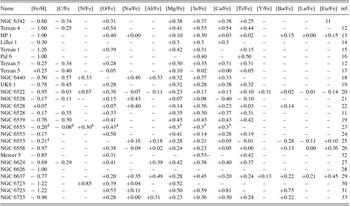
Table 3 shows the chemical abundances for a subset of GCs from Table 1, that have available high spectral resolution abundance analyses.
Table 3. Metallicities and abundances from high-resolution spectroscopy. References: 11: Origlia, Valenti, & Rich Reference Origlia, Valenti and Rich2005a; 12: Origlia & Rich Reference Origlia and Rich2004; 13: Barbuy et al. Reference Barbuy2006, Reference Barbuy2015, Reference Barbuy2014; 14: Origlia, Rich, & Castro Reference Origlia, Rich and Castro2002; 15: Valenti et al. Reference Valenti, Origlia, Mucciarelli and Rich2015; 16: Lee, Carney, & Balachandran Reference Lee, Carney and Balachandran2004; 17: Origlia et al. Reference Origlia2011; 18: Origlia, Valenti, & Rich Reference Origlia, Valenti and Rich2008; 19: Origlia et al. Reference Origlia, Valenti, Rich and Ferraro2005b; 20: Barbuy et al. Reference Barbuy2014; 21: Zoccali et al. Reference Zoccali2004; 22: Carretta et al. Reference Carretta, Cohen, Gratton and Behr2001; 23: Meléndez et al. Reference Meléndez2003 plus Origlia et al. Reference Origlia, Rich and Castro2002; 24: Cohen et al. Reference Cohen, Gratton, Behr and Carretta1999; 25: Alves-Brito et al. Reference Alves-Brito2006; 26: Barbuy et al. Reference Barbuy2007; 27: Valenti, Origlia, & Rich Reference Valenti, Origlia and Rich2011; 28: Smith & Wehlau Reference Smith and Wehlau1985; 29: Lee Reference Lee2007; 30: Gratton et al. Reference Gratton2015 for BHB; 31: Gratton et al. Reference Gratton2015 for RHB; 32: Peñaloza et al. Reference Peñaloza2015; 33 Rojas-Arriagada et al. Reference Rojas-Arriagada2016.
Carbon and Nitrogen: C and N show the expected anticorrelation due to CNO processing along the red giant branch. Two clusters with low N abundances should be further studied since this is not expected.
Odd-Z elements Na, Al A crucial issue concerns possible Na-O anticorrelation, which would indicate the presence of a second stellar generation. As a matter of fact, most GCs are presently being found to have at least two stellar generations, except possibly the least massive clusters. A threshold in mass for a second generation not to occur is presently estimated to be at 3–4 × 10⁴ M○ (R.G. Gratton, private communication), or in other words, essentially all GCs should show the Na-O anticorrelation. The second generation is detected via Na-O, Mg-Al anticorrelations, and also by the presence of both CN-strong and CN-weak stars (Carretta et al. Reference Carretta2009). The origin of these chemical anomalies is probably hot bottom burning (HBB) (Ventura et al. Reference Ventura, Di Criscienzo, Carini and D’Antona2013) in massive Asymptotic Giant Branch (AGB) first generation stars, with yields ejected in the internal cluster medium, and incorporated by the second generation stars, the latter showing these anomalies. A thorough discussion on the origin of multiple stellar populations in GCs is given in Renzini et al. (Reference Renzini2015). From Table 3, we see that very few of the bulge clusters were investigated in terms of Na and Al. In fact, four stars analysed by Barbuy et al. (Reference Barbuy2014) show no Na-O anticorrelation (see their Figure 6), however, more stars have to be analysed for a firm conclusion. An important investigation on this matter was carried out by Gratton et al. (Reference Gratton2015), where 17 BHB and 30 RHB stars of NGC 6723 were analysed. It was found that RHB and intermediate-BHB stars appear to belong to a first generation, showing O-rich and Na-poor abundances, whereas the bluest of the BHB stars show lower oxygen and higher Na (four BHB stars show [O/Fe] = +0.23 and [Na/Fe] = +0.11), in contrast with the mean values given in Table 3. Gratton et al. (Reference Gratton2015) consider that extended blue HB stars might correspond to a second generation of lower mass stars.

Figure 6. Bulge sample (Table 1). Upper panel: in the X,Y plane; Lower panel: X,Z plane.
Alpha-elements O, Mg, Si, Ca, Ti : In Figure 7 are plotted the abundances of these alpha elements versus [Fe/H], including the abundances for the bulge sample, as given in Table 3, compared with abundances for 57 field bulge giant stars from Lecureur et al. (Reference Lecureur2007), Gonzalez et al. (Reference Gonzalez2011), and Barbuy et al. (Reference Barbuy2015), and 58 bulge dwarf stars from Bensby et al. (Reference Bensby2013). The oxygen abundances are as given in Barbuy et al. (Reference Barbuy2015), where they were revised with respect to Lecureur et al. (Reference Lecureur2007). Some discrepancy between the oxygen abundances from Barbuy et al. (Reference Barbuy2015) and Bensby et al. (Reference Bensby2013) can be explained by the facts that: Barbuy et al. analysed red giants, using the forbidden [OI]6300.31 Å line and Bensby et al. (Reference Bensby2013) analysed dwarfs, using the permitted triplet OI lines at 7771.94, 7774.16, 7775.39 Å lines. Solar oxygen abundances adopted were respectively ε(O) = 8.87 and 8.85 for Barbuy et al. and Bensby et al., which would tend to invert the small shift between the two sets results. All in all, given that the permitted OI lines are well-known to be subject to strong non-LTE effects, and tend to overestimate the oxygen abundances, we can consider that there is a good agreement between the two sets of oxygen abundances.

Figure 7. [O, Mg, Si, Ca, Ti/Fe] versus [Fe/H] for sample globular clusters, compared with field stars. Symbols: red triangles: sample globular clusters from Table 3; green circles: 56 bulge giants analysed by Lecureur et al. (Reference Lecureur2007), Barbuy et al. (Reference Barbuy2015) and Gonzalez et al. (Reference Gonzalez2011); magenta circles: microlensed bulge dwarfs analysed by Bensby et al. (Reference Bensby2013). For Terzan 5, NGC 6528, NGC 6553, and NGC 6723, 2, 3, 3, and 2 sets of values are included, respectively.
The panels in Figure 7 indicate therefore that the alpha-elements O, Mg, Si, and Ca are overabundant by about [O, Mg, Si, Ca, Ti/Fe] ≈ 0.3 to 0.4 dex for the more metal-poor stars. The same is found for the field (see also Alves-Brito et al. Reference Alves-Brito, Meléndez, Asplund, Ramírez and Yong2010; Bensby et al. Reference Bensby2013). This implies early fast enrichment by core collapse supernovae SNII, which in turn give a short timescale for bulge formation, where even the metal-rich clusters are old (Ortolani et al. Reference Ortolani1995).
Heavy elements: Very few heavy element abundance derivation is available for individual stars of bulge GCs. The heavy elements of first peak Y, Sr, Zr, together with a few elements of the second peak Ba, La, and the r-element Eu, can reveal the nature of the first stars, or else to reveal if AGBs were acting as important chemical contributors. A threshold of about [Ba/Eu] = 0.6 would be indicative if Ba was produced by r- or s-process. If [Ba/Eu] > 0.6, this could be a hint of early enrichment by massive spinstars, and the same applies to the ratios Y/Ba, Sr/Ba, and Zr/Ba (Frischknecht et al. Reference Frischknecht2016). These ratios were studied for the GC NGC 6522, by Barbuy et al. (Reference Barbuy2009), Chiappini et al. (Reference Chiappini2011), and Ness, Asplund, & Casey (Reference Ness, Asplund and Casey2014) using GIRAFFE spectra from the survey by Zoccali et al. (Reference Zoccali2008). Barbuy et al. (Reference Barbuy2014) used new UVES spectra observed in 2012 for four of the same stars, and these new results are reported in Table 3. Sr lines are unreliable as shown by Barbuy et al. (Reference Barbuy2014), and Ness et al. (Reference Ness, Asplund and Casey2014), superseding abundance values given in Chiappini et al. (Reference Chiappini2011). Zr is difficult to derive: in Table 3, it is not reported given that it is only available for NGC 6522, but it is worth mentioning that Cantelli, Barbuy, Chiappini, Depagne, Pignatari, Hirschi, Ortolani, and Bica (in preparation) seems to detect a clear variation in Zr abundances among 12 member stars of NGC 6522 observed with GIRAFFE in 2012. The ratios from first to second peak of heavy elements can also be explained by production of s-process heavy elements in massive AGB stars, and predicted relative ratios between different heavy elements was presented in Bisterzo et al. (Reference Bisterzo2010, Reference Bisterzo2014). Finally, it is possible that all heavy elements in old stars were produced by the r-process only, as first suggested by Truran (Reference Truran1981).
5 KINEMATICS AND ORBITS
According to Minniti & Zoccali (Reference Minniti and Zoccali2008), the bulge kinematics as viewed from the field stars lies between a purely rotational system and a velocity dispersion supported one. Another important feature of stellar kinematics is the presence of a massive bar in the bulge (Blitz & Spergel Reference Blitz and Spergel1991). An X-shape of the bulge related to the box/peanut configuration has been suggested by McWilliam & Zoccali (Reference McWilliam and Zoccali2010) and Nataf et al. (Reference Nataf, Udalski, Gould, Fouqué and Stanek2010), from the double red clump detected in the near-IR CMDs of the bulge fields. This is interpreted as secular evolution of bars (e.g. Athanassoula Reference Athanassoula2005) and leads to the idea that the galactic bulge is not a classical bulge. This issue is developed in other reviews in this volume. Observations of the X-shape profile are detailed thoroughly in Wegg, Gerhard, & Portail (Reference Wegg, Gerhard and Portail2015 and references therein). It is a generic feature of boxy bulges and is seen in many other galaxies (e.g. Bureau et al. Reference Bureau2006).
Even if the X-shape is a confirmed feature, it is interesting to point out a recent study by Lee, Joo, & Chung (Reference Lee, Joo and Chung2015), that suggests an alternative explanation based on the presence of two different populations with a second generation of stars helium-enhanced and more metal rich, having a brighter clump than the first, more metal-poor component. In this model, there is no need for a deviation from a classical bulge shape. This is basically the same framework currently accepted for the multi-population features in the massive galactic GCs. Some issues are still open in this new interpretation, such as the source and the efficiency of the enrichment mechanism and the needed yields for the second generation component, in a wide environment such as the Galactic bulge. Accurate kinematics of the two clumps (for example, from GAIA) could disentangle between the two scenarios.
5.1. Bulge field properties
Kinematics. Babusiaux et al. (Reference Babusiaux2010, Reference Babusiaux2014) carried out a kinematical study of 650 bulge field stars, and concluded that the more metal-poor stars, where a lower end at around [Fe/H] ≈ −1.0 was found, correspond to a spheroidal distribution. The metal-rich stars showed instead a kinematics typical of the bar (see also review by Gonzalez & Gadotti Reference Gonzalez, Gadotti, Laurikainen, Peletier and Gadotti2016). Vásquez et al. (Reference Vásquez2013) studied the kinematics of 454 field bulge stars located in the bright and the faint red clumps of the X-shaped bulge. They conclude that stars with elongated orbits tend to be metal-poor, whereas the metal-rich ones are preferentially in axisymmetric orbits, at odds with conclusions by Babusiaux et al. (Reference Babusiaux2010).
Ages. Clarkson et al. (Reference Clarkson2008, Reference Clarkson2011) used proper motion cleaned data, deriving a cleaned bulge CMD, demonstrated to consist of an old population of at least 10 Gyr. The same conclusion had been reached previously by Zoccali et al. (Reference Zoccali2003).
5.2. Kinematics and orbits of bulge GCs
Space velocities for the GCs, that require radial velocities and proper motions to be derived, are only available for part of the sample. Tables 1 and 2 gather space velocities with respect to the Sun, and corresponding references. These space velocities, which result from a combination of radial velocities and proper motions, are reported in column 12 of Table 1 and column 8 of Table 2. Earlier work was carried out by Dinescu et al. (Reference Dinescu, Girard and van Altena1997, Reference Dinescu, van Altena and Girard1999a,Reference Dinescu, Girard and van Altena1999b, Reference Dinescu, Girard, van Altena and López2003) and Casetti-Dinescu et al. (Reference Casetti-Dinescu2007, Reference Casetti-Dinescu2010, Reference Casetti-Dinescu2013). Using HST data, Zoccali et al. (Reference Zoccali2003) and Feltzing & Johnson (Reference Feltzing and Johnson2002) derived space velocities for the metal-rich clusters NGC 6553 and NGC 6528, respectively. Rossi et al. (Reference Rossi2015) measured proper motion cleaned CMDs from long time base data, and derived space velocities for 10 central GCs.
An important piece of information was revealed by the orbits of the inner GCs derived by Rossi et al. (in preparation): all GCs located in the inner bulge appear to be trapped in the bar (Rossi et al. Reference Rossi2015; Rossi et al., in preparation). We point out that the clusters, in particular, the moderately metal-poor ones, probably formed very early in the very central parts of the Galaxy (e.g. NGC 6522, NGC 6558), before the bar instability occurred. This is confirmed by their rotational velocity counter-rotating with respect to the bar and the Galaxy in some cases. Since these clusters have low heights z, their retrograde orbits can be considered as robust with respect to variations of the bar shape (Pfenniger Reference Pfenniger1984). Therefore, it seems that whenever the bar formed, given their low kinematics, essentially all GCs would be trapped. Martinez-Valpuesta, Shlosman, & Heller (Reference Martinez-Valpuesta, Shlosman and Heller2006) suggested that a first vertical buckling of the growing bar occurred at 1.8–2.8 Gyr, and a second at 6–7.5 Gyr. The bar then assumes a boxy or peanut X-shape. The trapping of GCs in the boxy bulge includes bulge clusters of all metallicities, from moderately metal-poor as mentioned above, to metal-rich ones like Terzan 2.
A main conclusion is that the inner clusters are confined and possibly trapped in the bar, due to the high mass of the bar, achievable due to the low velocity components of the clusters.
6 FUTURE STEPS
Figure 5 shows the GCs projected in the central ‖l‖ < 8° and ‖b‖ < 5°. These include the sample by Barbuy et al. (Reference Barbuy, Bica and Ortolani1998), which was given in a radius of R < 5°, and a few more, in particular, Terzan 9, Al 3, and results from the VVV survey. The VVV survey provided new GCs and candidates in that region (Borissova et al. Reference Borissova2011, Reference Borissova2014). The clusters VVV CL001, CL 002, CL 003, and CL 004 were studied by means of the VVV photometric catalogue (Minniti et al. Reference Minniti2011, Moni Bidin et al. Reference Moni Bidin2011). VVV CL 002 appears to be the most central GC. VVV CL 001 is projected very close to UKS 1 and they may be a binary system (Minniti et al. Reference Minniti2011). In this case, UKS 1 might be interpreted as a dwarf galaxy remains, similarly to Terzan 5. VVV CL 003 seems to be a far side GC or old open cluster, while VVV CL 004 might be rather an old open cluster. Table 4 shows available information on the VVV sample, including ages and GC candidates (Borissova et al. Reference Borissova2014). Table 4 reveals a number of candidates in zones where 2MASS and GLIMPSE could not detect clusters. These previous surveys showed GCs outside the central bulge only.
Table 4. VVV GCs and candidates. References: 1: Minniti et al. (Reference Minniti2011); 2: Moni Bidin et al. (Reference Moni Bidin2011); 3: Borissova et al. (Reference Borissova2014).

Figure 5 shows the angular distribution of known GCs projected in the central parts of the Galaxy, and candidate ones found in the VVV survey. This figure, together with Table 1, clearly show the depletion of GCs on the far side. Besides, VVV CL 002 is very close to the Galactic centre, and VVV CL 003 is in the far size. The VVV candidates (Table 4) may mitigate that asymmetric distribution, but will not completely solve the problem of missing GCs in the far side. We recall, however, that when IR distances are taken into account, the clusters are well distributed around 8 kpc (Section 3).
Ivanov, Kurtev, & Borissova (Reference Ivanov, Kurtev and Borissova2005) estimated that in the central parts of the Galaxy at least 10 ± 3 GCs were missing. Several new GCs have been discovered or identified as such in the last decade, especially with observations in the near IR, in the area outside Figure 5, and recently, in the inner bulge region VVV CL 002 has been added. The VVV candidates are a promising sample to further populate the inner bulge.
Figure 5 portrays the current status of the inner bulge sample, together with VVV GCs and candidates (Table 1). As pointed out by Barbuy et al. (Reference Barbuy, Bica and Ortolani1998), a zone of avoidance in the GC distribution occurs for 0.9 < b < − 1.9. It is related to dust heavily absorbing in the disk and/or dynamical effects on the GC population by the disk (bar) and bulge. The zone of avoidance is asymmetric in Galactic latitude because of the Sun's offset of about 18 pc above the Galactic plane. The zone of avoidance now includes 5 VVV candidates (Figure 5), while the other ones are distributed as in the sample available previously in Barbuy et al. (Reference Barbuy, Bica and Ortolani1998).
Finally, as concerns a possible binarity between VVV CL 001 and UKS 1, it is interesting to note that, likewise, the halo dwarf spheroidal Ursa Minor has a GC companion (Muñoz et al. Reference Muñoz2012). Growing evidence suggests that a fraction of the inner bulge sample are galaxy remains. In the coming years, Gaia may show streamers related to them, to further constrain the dynamical issues involved.
7 CONCLUSIONS
In this review, we provide a state-of-the-art list of bulge GCs and their properties. We tried to constrain their properties including their kinematics when available. Kinematics is becoming a key tool to identify their nature, and the link with the field stellar populations, within the complex substructures of the bulge.
In recent years, good progress in the knowledge of the GCs in the central parts of the Galaxy has been achieved. For spectroscopy, the multi-object spectrographs in 8 m-class telescopes have made it possible to derive chemical abundances for considerable numbers of stars. Progress in instrumentation thanks to imaging with MCAO in the infrared (MAD/VLT, GEMS/Gemini) and HST/NICMOS, has made possible long time baseline of CCD data with excellent quality, allowing proper motion cleaning of CMDs. Finally, surveys with larger apertures such as the 4 m VISTA Telescope provided the discovery of new objects. The VVV survey in particular has provided several new bulge globular clusters and candidates, to be explored in coming years.
Much work is still needed as concerns bulge globular clusters, such as the monitoring of variable stars, in particular RR Lyrae, to obtain deep CMDs allowing age derivation, and the derivation of metallicities and chemical abundances from high-resolution spectroscopy. The derivation of Na and O abundances will be crucial to define if these very old clusters have a unique or multiple stellar generations. These results should allow to better compare the bulge globular clusters with outer bulge, inner halo, and outer halo ones.
ACKNOWLEDGEMENTS
EB and BB acknowledge partial financial support from CNPq, CAPES, and Fapesp. SO acknowledges the Italian Ministero dell’Università e della Ricerca Scientifica e Tecnologica (MURST), Italy.


 Open access