


1 Introduction
Light-by-light scattering is a purely quantum effect (Halpern Reference Halpern1933; Euler & Kockel Reference Euler and Kockel1935; Heisenberg & Euler Reference Heisenberg and Euler1936) which contributes to e.g. the electron magnetic moment, the Lamb shift and Delbrück scattering. In these cases virtual, or both virtual and real, photons are involved, while light-by-light scattering of only real photons has not yet been observed.
While the word ‘scattering’ suggests momentum change, one manifestation of light-by-light effects is the near-forward scattering of photons with changes to internal degrees-of-freedom, i.e. helicity (or polarisation). Consider the collision of two linearly polarised laser pulses, the first a high-intensity optical pulse, the ‘target’, the second a low-intensity X-ray pulse, the ‘probe’ (Heinzl et al. Reference Heinzl, Liesfeld, Amthor, Schwoerer, Sauerbrey and Wipf2006). Due to the separation in energy scales the probe beam essentially scatters forward, but quantum effects can still cause probe photons to change helicity state. This manifests macroscopically as a slight ellipticity in the probe beam and is hence known as ‘vacuum birefringence’ in analogy to the ellipticity induced in a beam of light passing through a birefringent crystal (Toll Reference Toll1952). Indeed, many phenomena in nonlinear optics have purely photonic analogues, see Di Piazza, Hatsagortsyan & Keitel (Reference Di Piazza, Hatsagortsyan and Keitel2006), Heinzl et al. (Reference Heinzl, Liesfeld, Amthor, Schwoerer, Sauerbrey and Wipf2006), Marklund & Shukla (Reference Marklund and Shukla2006), King, Di Piazza & Keitel (Reference King, Di Piazza and Keitel2010), Kim & Lee (Reference Kim and Lee2011), Gies, Karbstein & Seegert (Reference Gies, Karbstein and Seegert2013) and Gies, Karbstein & Seegert (Reference Gies, Karbstein and Seegert2015).
The measurement of vacuum birefringence has been selected as a flagship experiment by the HiBEF consortium at DESY (HIBEF 2015; Schlenvoigt et al. Reference Schlenvoigt, Heinzl, Schramm, Cowan and Sauerbrey2016), following the proposal in Heinzl et al. (Reference Heinzl, Liesfeld, Amthor, Schwoerer, Sauerbrey and Wipf2006). For a recent review of the theory behind this topic, see King & Heinzl (Reference King and Heinzl2015) and for a detailed review of the current experimental status, see Schlenvoigt et al. (Reference Schlenvoigt, Heinzl, Schramm, Cowan and Sauerbrey2016).
In this paper we will investigate two alternative, but related, set-ups which have been suggested for measuring light-by-light effects with real photons. Our goal is simply to obtain a very rough idea of how promising these two alternative schemes are: if they seem promising, the calculations presented here can be refined. The first set-up replaces the intense optical laser above with an alternative target, namely an optimally focused ‘dipole pulse’ (Gonoskov et al. Reference Gonoskov, Aiello, Heugel and Leuchs2012). The second set-up retains the intense optical pulse as target, but replaces the above X-ray probe with high-energy photons (gamma rays) emitted as synchrotron radiation from a laser–particle collision. This is the proposed set-up for measuring helicity-changing processes at the ELI-NP facility in Romania (ELI 2014; Nakamiya et al. Reference Nakamiya, Homma, Moritaka and Seto2015).
This paper is organised as follows. In § 2 we describe our approach. In § 3 we consider the alternative target set-up. In § 4 we consider the alternative probe and describe the proposed experimental implementation of such a set-up at ELI-NP. We conclude in § 5.
2 Helicity flip in background fields
Recall the standard optics result for the polarisation ellipticity
 ${\it\delta}$
induced in a beam of light, frequency
${\it\delta}$
induced in a beam of light, frequency
 ${\it\omega}^{\prime }$
, passing through a birefringent medium of length
${\it\omega}^{\prime }$
, passing through a birefringent medium of length
 $d$
, refractive indices
$d$
, refractive indices
 $\{n_{+},n_{-}\}$
:
$\{n_{+},n_{-}\}$
:
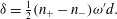 $$\begin{eqnarray}{\it\delta}={\textstyle \frac{1}{2}}(n_{+}-n_{-}){\it\omega}^{\prime }d.\end{eqnarray}$$
The quantum vacuum exposed to a strong field effectively develops ‘vacuum refractive indices’ which arise through the nonlinearity of the Euler–Heisenberg action (Euler & Kockel Reference Euler and Kockel1935; Heisenberg & Euler Reference Heisenberg and Euler1936), and can be calculated using the photon polarisation tensor. In the limit that the strong field is a constant, homogeneous crossed field of strength
 $E$
, a counter-propagating probe sees the indices (Toll Reference Toll1952; Narozhny Reference Narozhny1969)
$E$
, a counter-propagating probe sees the indices (Toll Reference Toll1952; Narozhny Reference Narozhny1969)
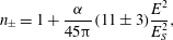 $$\begin{eqnarray}n_{\pm }=1+\frac{{\it\alpha}}{45{\rm\pi}}(11\pm 3)\frac{E^{2}}{E_{S}^{2}},\end{eqnarray}$$
where
 $E_{S}=m^{2}/e\simeq 10^{18}~\text{V}~\text{m}^{-1}$
is the Sauter–Schwinger field. Inserting (2.2) into (2.1) we obtain the ellipticity induced in the probe as
$E_{S}=m^{2}/e\simeq 10^{18}~\text{V}~\text{m}^{-1}$
is the Sauter–Schwinger field. Inserting (2.2) into (2.1) we obtain the ellipticity induced in the probe as
 $$\begin{eqnarray}{\it\delta}\rightarrow \frac{{\it\alpha}}{15{\rm\pi}}\frac{E^{2}}{E_{S}^{2}}{\it\omega}^{\prime }d.\end{eqnarray}$$
This macroscopic beam ellipticity induced by quantum effects is ‘vacuum birefringence’; the microscopic physics underlying it is as follows.
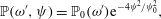
Consider a probe photon, momentum
 $l_{{\it\mu}}\equiv {\it\omega}^{\prime }\hat{l}_{{\it\mu}}$
, frequency
$l_{{\it\mu}}\equiv {\it\omega}^{\prime }\hat{l}_{{\it\mu}}$
, frequency
 ${\it\omega}^{\prime }$
and helicity state described by
${\it\omega}^{\prime }$
and helicity state described by
 ${\it\epsilon}_{{\it\mu}}$
. The photon passes through a strong background field
${\it\epsilon}_{{\it\mu}}$
. The photon passes through a strong background field
 $\unicode[STIX]{x1D60D}_{{\it\mu}{\it\nu}}$
with typical frequency scale much smaller than
$\unicode[STIX]{x1D60D}_{{\it\mu}{\it\nu}}$
with typical frequency scale much smaller than
 ${\it\omega}^{\prime }$
(as would be the case for an X-ray probe of an optical laser). In this case scattering becomes essentially forward. The probability
${\it\omega}^{\prime }$
(as would be the case for an X-ray probe of an optical laser). In this case scattering becomes essentially forward. The probability
 $\mathbb{P}$
that the probe photon flips to its opposite helicity state
$\mathbb{P}$
that the probe photon flips to its opposite helicity state
 ${\it\epsilon}_{{\it\mu}}^{\prime }$
may be written
${\it\epsilon}_{{\it\mu}}^{\prime }$
may be written
 $\mathbb{P}_{flip}=|\mathbb{T}|^{2}$
, where the amplitude
$\mathbb{P}_{flip}=|\mathbb{T}|^{2}$
, where the amplitude
 $\mathbb{T}$
can be approximated by a line integral over the classical (i.e. straight line) trajectory of the photon (Dinu et al.
Reference Dinu, Heinzl, Ilderton, Marklund and Torgrimsson2014a
), here parameterised with time
$\mathbb{T}$
can be approximated by a line integral over the classical (i.e. straight line) trajectory of the photon (Dinu et al.
Reference Dinu, Heinzl, Ilderton, Marklund and Torgrimsson2014a
), here parameterised with time
 $t$
:
$t$
:
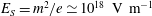
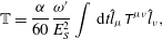
 $$\begin{eqnarray}\mathbb{T}=\frac{{\it\alpha}}{30}\frac{{\it\omega}^{\prime }}{E_{S}^{2}}\int \,\text{d}t(\bar{{\it\epsilon}}_{{\it\mu}}^{\prime }\unicode[STIX]{x1D60D}^{{\it\mu}{\it\nu}}\hat{l}_{{\it\nu}})({\it\epsilon}_{{\it\sigma}}\unicode[STIX]{x1D60D}^{{\it\sigma}{\it\rho}}\hat{l}_{{\it\rho}}).\end{eqnarray}$$
 $\unicode[STIX]{x1D60D}_{{\it\mu}{\it\nu}}$
is evaluated on the photon trajectory. The probability is maximised when the field and probe polarisations can be chosen to lie at a relative angle of
$\unicode[STIX]{x1D60D}_{{\it\mu}{\it\nu}}$
is evaluated on the photon trajectory. The probability is maximised when the field and probe polarisations can be chosen to lie at a relative angle of
 $45^{\circ }$
.
$45^{\circ }$
.
 $\mathbb{T}$
then reduces to
$\mathbb{T}$
then reduces to
 $$\begin{eqnarray}\mathbb{T}=\frac{{\it\alpha}}{60}\frac{{\it\omega}^{\prime }}{E_{S}^{2}}\int \,\text{d}t\hat{l}_{{\it\mu}}\unicode[STIX]{x1D61B}^{{\it\mu}{\it\nu}}\hat{l}_{{\it\nu}},\end{eqnarray}$$
where
 $\unicode[STIX]{x1D61B}_{{\it\mu}{\it\nu}}$
is the background field energy–momentum tensor; thus we can interpret (2.5) as simply being proportional to an integrated energy density (an intensity) seen by the probe as it passes through the target (Dinu et al.
Reference Dinu, Heinzl, Ilderton, Marklund and Torgrimsson2014a
). That this is an integrated, rather than peak, variable will be important below.
$\unicode[STIX]{x1D61B}_{{\it\mu}{\it\nu}}$
is the background field energy–momentum tensor; thus we can interpret (2.5) as simply being proportional to an integrated energy density (an intensity) seen by the probe as it passes through the target (Dinu et al.
Reference Dinu, Heinzl, Ilderton, Marklund and Torgrimsson2014a
). That this is an integrated, rather than peak, variable will be important below.
As detailed in Dinu et al. (Reference Dinu, Heinzl, Ilderton, Marklund and Torgrimsson2014b
), the flip probability
 $\mathbb{P}$
is directly related to the ellipticity
$\mathbb{P}$
is directly related to the ellipticity
 ${\it\delta}^{2}$
: hence (2.4) is most easily interpreted as a quantum field theory generalisation of the classical result (2.1), which goes beyond (2.3) as it allows us to consider arbitrary field strengths and shapes (on the usual provisos that the field strength is not of Schwinger scale and the invariant, centre of mass (c.o.m.), frequency scales do not exceed the electron mass).
${\it\delta}^{2}$
: hence (2.4) is most easily interpreted as a quantum field theory generalisation of the classical result (2.1), which goes beyond (2.3) as it allows us to consider arbitrary field strengths and shapes (on the usual provisos that the field strength is not of Schwinger scale and the invariant, centre of mass (c.o.m.), frequency scales do not exceed the electron mass).
There are several effects which we do not include in this first investigation. No depletion of the background field is accounted for, nor do we account for probe scattering (Lundstrom et al. Reference Lundstrom, Brodin, Lundin, Marklund, Bingham, Collier, Mendonca and Norreys2006; King & Keitel Reference King and Keitel2012; Karbstein et al. Reference Karbstein, Gies, Reuter and Zepf2015), for an investigation of which in vacuum birefringence, see Karbstein et al. (Reference Karbstein, Gies, Reuter and Zepf2015). We also restrict our attention to single photon probes; beam-like probes can be accounted for using a straightforward extension of the formalism used here (Dinu et al. Reference Dinu, Heinzl, Ilderton, Marklund and Torgrimsson2014a ; Torgrimsson Reference Torgrimsson2015). In summary, our current approximation gives a good estimate for the on-axis birefringence signal. (Note though that in experiments with either laser or magnetic fields scattered photon signals may be easier to detect than on-axis signals, due to lower backgrounds (Gies et al. Reference Gies, Karbstein and Seegert2013; Karbstein Reference Karbstein2015; Karbstein et al. Reference Karbstein, Gies, Reuter and Zepf2015).)
2.1 Conventions and notation
The helicity-state vectors for a photon of momentum
 $l_{{\it\mu}}$
are
$l_{{\it\mu}}$
are
 $$\begin{eqnarray}{\it\epsilon}_{\pm }^{{\it\mu}}=\frac{1}{\sqrt{2}}({\it\epsilon}_{1}^{{\it\mu}}\pm \text{i}{\it\epsilon}_{2}^{{\it\mu}}),\end{eqnarray}$$
where, using Coulomb gauge,
 $$\begin{eqnarray}\displaystyle & l^{{\it\mu}}={\it\omega}^{\prime }(1,\sin {\it\theta}\cos {\it\phi},\sin {\it\theta}\sin {\it\phi},\cos {\it\phi}), & \displaystyle\end{eqnarray}$$
 $$\begin{eqnarray}\displaystyle & {\it\epsilon}_{1}^{{\it\mu}}=(0,\cos {\it\theta}\cos {\it\phi},\cos {\it\theta}\sin {\it\phi},-\hspace{-2.0pt}\sin {\it\phi}), & \displaystyle\end{eqnarray}$$
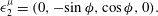 $$\begin{eqnarray}\displaystyle & {\it\epsilon}_{2}^{{\it\mu}}=(0,-\hspace{-2.0pt}\sin {\it\phi},\cos {\it\phi},0). & \displaystyle\end{eqnarray}$$
3 Dipole pulse targets
Dipole pulses are exact, singularity free, optimally focussed, finite-energy solutions of Maxwell’s equations in a vacuum (Gonoskov et al.
Reference Gonoskov, Aiello, Heugel and Leuchs2012). In an ‘
 $e$
-dipole’ pulse the electric field dominates over the magnetic field in the focus, and provides optimal conditions for pair production via the non-perturbative Sauter–Schwinger mechanism (Gonoskov et al.
Reference Gonoskov, Gonoskov, Harvey, Ilderton, Kim, Marklund, Mourou and Sergeev2013, Reference Gonoskov, Bashinov, Gonoskov, Harvey, Ilderton, Kim, Marklund, Mourou and Sergeev2014). In an ‘
$e$
-dipole’ pulse the electric field dominates over the magnetic field in the focus, and provides optimal conditions for pair production via the non-perturbative Sauter–Schwinger mechanism (Gonoskov et al.
Reference Gonoskov, Gonoskov, Harvey, Ilderton, Kim, Marklund, Mourou and Sergeev2013, Reference Gonoskov, Bashinov, Gonoskov, Harvey, Ilderton, Kim, Marklund, Mourou and Sergeev2014). In an ‘
 $h$
-dipole’ pulse, the magnetic field dominates and one might ask whether the optimal focussing amplifies the helicity-flip probability. To investigate this we consider replacing the intense beam in the vacuum birefringence experiments described above with an
$h$
-dipole’ pulse, the magnetic field dominates and one might ask whether the optimal focussing amplifies the helicity-flip probability. To investigate this we consider replacing the intense beam in the vacuum birefringence experiments described above with an
 $h$
-dipole pulse.
$h$
-dipole pulse.
The fields of an
 $h$
-dipole pulse are written in terms of a function
$h$
-dipole pulse are written in terms of a function
 $\boldsymbol{Z}$
defined by
$\boldsymbol{Z}$
defined by
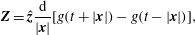 $$\begin{eqnarray}\boldsymbol{Z}=\hat{\boldsymbol{z}}\frac{\text{d}}{|\boldsymbol{x}|}[g(t+|\boldsymbol{x}|)-g(t-|\boldsymbol{x}|)],\end{eqnarray}$$
where the ‘driving function’
 $g$
will be specified shortly and the ‘virtual dipole moment’
$g$
will be specified shortly and the ‘virtual dipole moment’
 $d$
is a constant. The fields are
$d$
is a constant. The fields are
 $$\begin{eqnarray}\boldsymbol{B}=-\boldsymbol{{\rm\nabla}}\times \boldsymbol{{\rm\nabla}}\times \boldsymbol{Z},\quad \boldsymbol{E}=\boldsymbol{{\rm\nabla}}\times \dot{\boldsymbol{Z}},\end{eqnarray}$$
and in the focus are equal to
 $$\begin{eqnarray}\boldsymbol{B}(0,t)=\hat{\boldsymbol{z}}\frac{4d}{3}\dddot{g}(t),\quad \boldsymbol{E}(0,t)=0.\end{eqnarray}$$
For the driving function we choose a Gaussian,
 $$\begin{eqnarray}g(t)=\text{e}^{-{\rm\Delta}{\it\omega}^{2}t^{2}/4}\sin ({\it\omega}t),\end{eqnarray}$$
in which
 ${\it\omega}$
is the central frequency and
${\it\omega}$
is the central frequency and
 ${\rm\Delta}{\it\omega}$
is a frequency spread. In the focus we have, from (3.3a,b
), the same frequency spread as in
${\rm\Delta}{\it\omega}$
is a frequency spread. In the focus we have, from (3.3a,b
), the same frequency spread as in
 $g$
. The intensity distribution of the dipole pulse has the form (Gonoskov et al.
Reference Gonoskov, Aiello, Heugel and Leuchs2012)
$g$
. The intensity distribution of the dipole pulse has the form (Gonoskov et al.
Reference Gonoskov, Aiello, Heugel and Leuchs2012)
 $$\begin{eqnarray}I=I_{0}\sin ^{2}{\it\theta},\end{eqnarray}$$
where
 ${\it\theta}$
is the angle made with the
${\it\theta}$
is the angle made with the
 $z$
-axis.
$z$
-axis.
We will compare the flip probability in a dipole pulse with that in a Gaussian (paraxial) beam of the same input energy, using the expected parameters for the petawatt (PW) laser at DESY in conjunction with birefringence experiments (Schlenvoigt et al.
Reference Schlenvoigt, Heinzl, Schramm, Cowan and Sauerbrey2016). We take a total energy of 30 J, wavelength
 ${\it\lambda}=800~\text{nm}$
and a bandwidth of
${\it\lambda}=800~\text{nm}$
and a bandwidth of
 ${\rm\Delta}{\it\omega}\simeq 0.035{\it\omega}$
(corresponding to a FWHM pulse duration 28 fs). For the Gaussian we also need to choose a focal spot radius, which we take to be
${\rm\Delta}{\it\omega}\simeq 0.035{\it\omega}$
(corresponding to a FWHM pulse duration 28 fs). For the Gaussian we also need to choose a focal spot radius, which we take to be
 $w_{0}=1.75~{\rm\mu}\text{m}$
, again following Schlenvoigt et al. (Reference Schlenvoigt, Heinzl, Schramm, Cowan and Sauerbrey2016).
$w_{0}=1.75~{\rm\mu}\text{m}$
, again following Schlenvoigt et al. (Reference Schlenvoigt, Heinzl, Schramm, Cowan and Sauerbrey2016).
For these parameters the peak fields in the foci of the dipole and Gaussian beams become
 $$\begin{eqnarray}{\textstyle \frac{1}{2}}(\boldsymbol{E}^{2}+\boldsymbol{B}^{2})\simeq \left\{\begin{array}{@{}ll@{}}3\times 10^{-6}E_{S}^{2}\quad & \text{Dipole},\\ 9\times 10^{-8}E_{S}^{2}\quad & \text{Gaussian},\end{array}\right.\end{eqnarray}$$
differing by over an order of magnitude: we may therefore expect a significantly stronger birefringence signal in the dipole pulse than in the Gaussian beam. However other factors also play a roll, e.g. polarisation alignment between probe and target (the dipole pulse is radially polarised). Turning to the flip probability (2.4) or (2.5) we also need a probe photon trajectory. We consider the best possible scenario where the probe passes through the field focus (i.e. zero impact parameter) at the instant of peak field strength (i.e. no timing miss). The resulting probabilities (naturally) follow the intensity profiles of the background fields. That in the dipole, for example, follows (3.5) and has the form
 $$\begin{eqnarray}|\mathbb{T}_{flip}|^{2}=C_{0}\sin ^{4}{\it\theta},\end{eqnarray}$$
where the incoming probe makes an angle
 ${\it\theta}$
to the
${\it\theta}$
to the
 $z$
-axis and
$z$
-axis and
 $C_{0}$
depends on the dipole pulse parameters and probe frequency, but not on
$C_{0}$
depends on the dipole pulse parameters and probe frequency, but not on
 ${\it\theta}$
or polarisation angles.
${\it\theta}$
or polarisation angles.
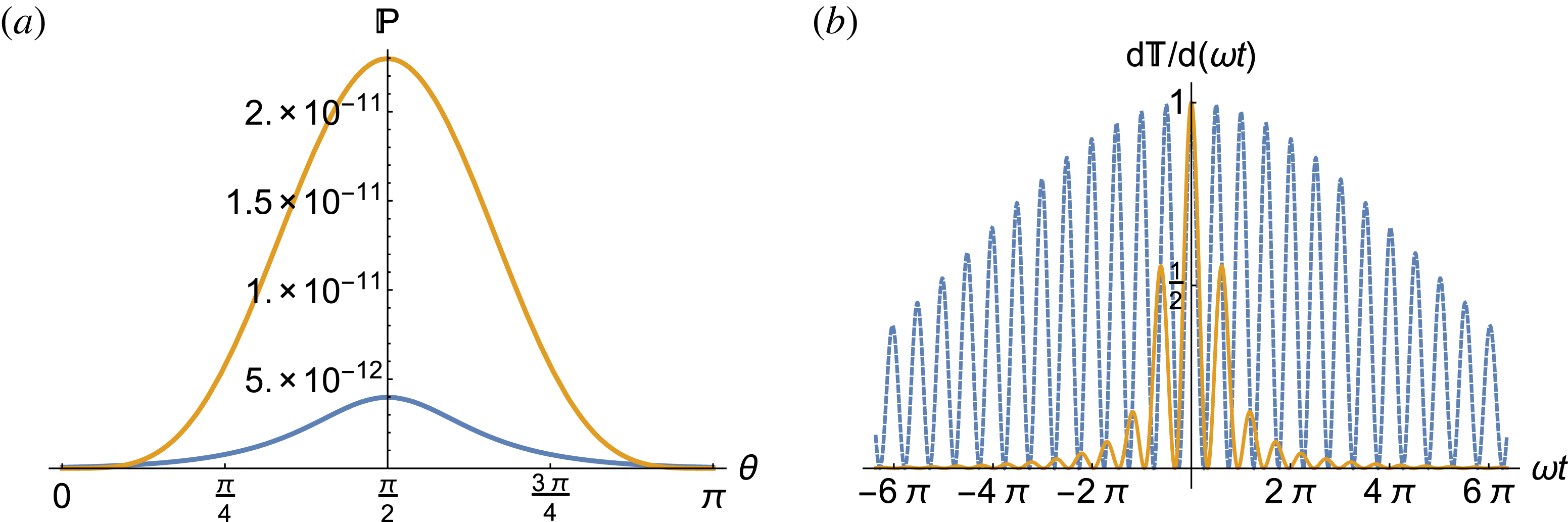
Figure 1. (a) Helicity-flip probability
 $\mathbb{P}$
in the dipole (yellow) and Gaussian (blue, with
$\mathbb{P}$
in the dipole (yellow) and Gaussian (blue, with
 ${\it\theta}$
shifted by
${\it\theta}$
shifted by
 ${\rm\pi}/2$
to be able to plot on the same scale). (b) The integrands of the normalised probability amplitudes
${\rm\pi}/2$
to be able to plot on the same scale). (b) The integrands of the normalised probability amplitudes
 $\mathbb{T}$
; in the Gaussian the focal spot is larger, and it can be seen that
$\mathbb{T}$
; in the Gaussian the focal spot is larger, and it can be seen that
 $\mathbb{T}$
indeed receives contributions from a larger time interval.
$\mathbb{T}$
indeed receives contributions from a larger time interval.
Further explicit expressions are unrevealing – instead we plot in figure 1 the flip probability in the dipole pulse and in the Gaussian beam. The probability in the dipole pulse exceeds that in the Gaussian by a factor of approximately 5.8, which is less than might be expected from (3.6). The reason for this is seen by recalling that it is an integrated parameter to which birefringence is sensitive, and that while the focal field strength in a dipole pulse is higher than in a Gaussian, the spot size is smaller. We can confirm this by estimating the effective transverse extent of the focus in our dipole pulse (transverse since the best case scenario is for probe angle
 ${\it\theta}={\rm\pi}/2$
). Following Gonoskov et al. (Reference Gonoskov, Aiello, Heugel and Leuchs2012) we define the effective extent as the distance from the focal point at which the energy density drops to half its peak value. For our parameters we find a sub-wavelength extent
${\it\theta}={\rm\pi}/2$
). Following Gonoskov et al. (Reference Gonoskov, Aiello, Heugel and Leuchs2012) we define the effective extent as the distance from the focal point at which the energy density drops to half its peak value. For our parameters we find a sub-wavelength extent
 $\simeq 0.4{\it\lambda}$
. In figure 1(a), we plot the (normalised) integrands of
$\simeq 0.4{\it\lambda}$
. In figure 1(a), we plot the (normalised) integrands of
 $\mathbb{T}$
in the dipole and Gaussian beams. We clearly see that the probability amplitude receives contributions from a much larger phase range in a Gaussian beam than it does in a dipole pulse; for the dipole case the width of the central peak is roughly
$\mathbb{T}$
in the dipole and Gaussian beams. We clearly see that the probability amplitude receives contributions from a much larger phase range in a Gaussian beam than it does in a dipole pulse; for the dipole case the width of the central peak is roughly
 $0.4{\it\lambda}$
, consistent with expectations.
$0.4{\it\lambda}$
, consistent with expectations.
4 Synchrotron emission as a probe
Above we discussed an ‘alternative target’ for measuring vacuum birefringence. We now turn to an ‘alternative probe’, namely synchrotron emission. We begin by recalling some standard results (Duke Reference Duke2000). The spectral density of synchrotron emission from a particle with gamma factor
 ${\it\gamma}$
moving in planar circular motion, radius
${\it\gamma}$
moving in planar circular motion, radius
 $R$
, is
$R$
, is
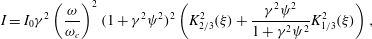 $$\begin{eqnarray}I=I_{0}{\it\gamma}^{2}\left(\frac{{\it\omega}}{{\it\omega}_{c}}\right)^{2}(1+{\it\gamma}^{2}{\it\psi}^{2})^{2}\left(K_{2/3}^{2}({\it\xi})+\frac{{\it\gamma}^{2}{\it\psi}^{2}}{1+{\it\gamma}^{2}{\it\psi}^{2}}K_{1/3}^{2}({\it\xi})\right),\end{eqnarray}$$
where the critical frequency is
 ${\it\omega}_{c}=3{\it\gamma}^{3}/2R$
,
${\it\omega}_{c}=3{\it\gamma}^{3}/2R$
,
 ${\it\psi}$
is the angle of elevation out of the plane of motion,
${\it\psi}$
is the angle of elevation out of the plane of motion,
 ${\it\xi}=({\it\omega}/{\it\omega}_{c})(1+{\it\gamma}^{2}{\it\psi}^{2})^{3/2}$
and
${\it\xi}=({\it\omega}/{\it\omega}_{c})(1+{\it\gamma}^{2}{\it\psi}^{2})^{3/2}$
and
 $I_{0}$
is an overall normalisation which is not important here. The two terms in the large brackets of (4.1) represent, respectively, the intensities radiated parallel and perpendicular to the plane of motion, which we write as
$I_{0}$
is an overall normalisation which is not important here. The two terms in the large brackets of (4.1) represent, respectively, the intensities radiated parallel and perpendicular to the plane of motion, which we write as
 $I_{\Vert }$
and
$I_{\Vert }$
and
 $I_{\bot }$
. Synchrotron radiation is highly plane polarised, as illustrated in figure 2. The small-angle part of the spectrum is therefore a potential source of highly polarised photons for use in birefringence experiments: if these photons interact with an intense optical pulse, helicity flip will mix the plane and perpendicularly polarised parts of the emitted radiation, ‘deforming’ the synchrotron spectrum. (Of course we need a high-energy synchrotron spectrum to obtain an appreciable flip probability, see below.)
$I_{\bot }$
. Synchrotron radiation is highly plane polarised, as illustrated in figure 2. The small-angle part of the spectrum is therefore a potential source of highly polarised photons for use in birefringence experiments: if these photons interact with an intense optical pulse, helicity flip will mix the plane and perpendicularly polarised parts of the emitted radiation, ‘deforming’ the synchrotron spectrum. (Of course we need a high-energy synchrotron spectrum to obtain an appreciable flip probability, see below.)
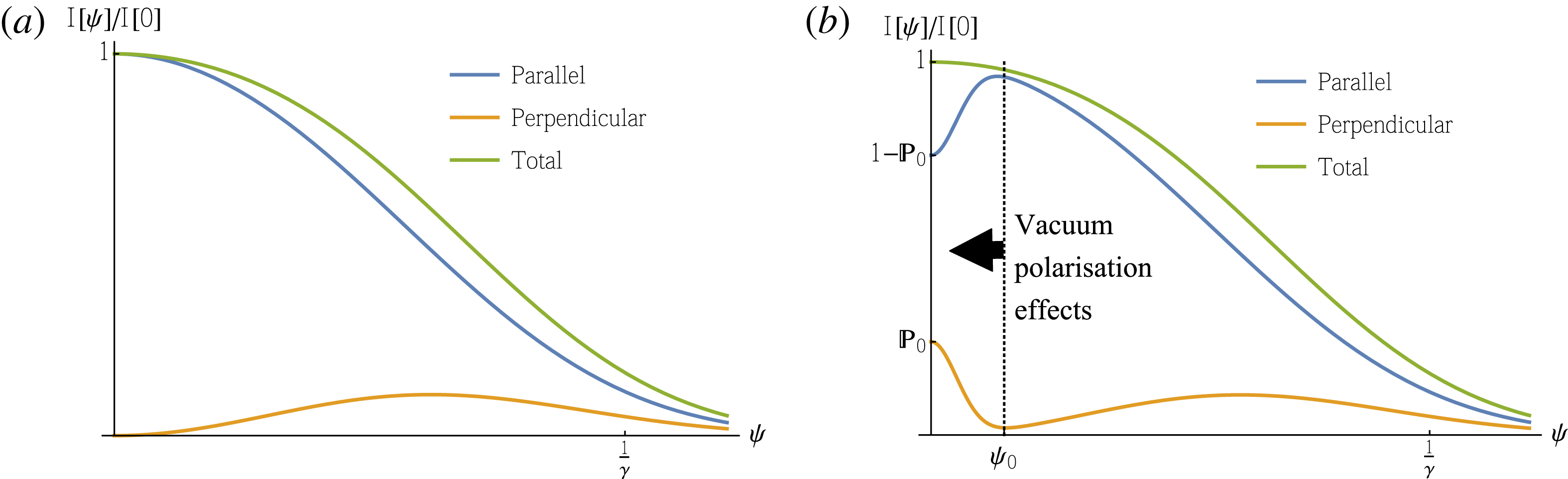
Figure 2. (a) Standard synchrotron emission spectrum as a function of opening angle
 ${\it\psi}$
at, to illustrate,
${\it\psi}$
at, to illustrate,
 ${\it\omega}^{\prime }=1.3{\it\omega}_{c}$
. The radiation is emitted in a narrow cone of opening angle
${\it\omega}^{\prime }=1.3{\it\omega}_{c}$
. The radiation is emitted in a narrow cone of opening angle
 ${\it\psi}\sim 1/{\it\gamma}$
. (b) The same spectrum illustrating the effects of vacuum polarisation, which are confined to narrower angles
${\it\psi}\sim 1/{\it\gamma}$
. (b) The same spectrum illustrating the effects of vacuum polarisation, which are confined to narrower angles
 ${\it\psi}\lesssim {\it\psi}_{0}$
defined by the interaction geometry. Photon helicity flip mixes the parallel and perpendicularly polarised components of the synchrotron spectrum.
${\it\psi}\lesssim {\it\psi}_{0}$
defined by the interaction geometry. Photon helicity flip mixes the parallel and perpendicularly polarised components of the synchrotron spectrum.
The portion of photons which will interact with the focal spot of the intense pulse is limited by the geometry of the experiment. Assume that the distance between the emission point of the high-energy photons and the focal point of the high-intensity pulse is
 $L$
, and that the pulse’s focal width is
$L$
, and that the pulse’s focal width is
 $w_{0}$
– see figure 3. Clearly only photons emitted in a very narrow angle
$w_{0}$
– see figure 3. Clearly only photons emitted in a very narrow angle
 ${\it\psi}<{\it\psi}_{0}:=\tan ^{-1}w_{0}/L$
will see the laser focal spot and be likely to change helicity stateFootnote
1
. This will be, as we verify below, much smaller than the typical opening angle (
${\it\psi}<{\it\psi}_{0}:=\tan ^{-1}w_{0}/L$
will see the laser focal spot and be likely to change helicity stateFootnote
1
. This will be, as we verify below, much smaller than the typical opening angle (
 $1/{\it\gamma}$
) of the synchrotron spectrum, so vacuum polarisation effects will only be observable for photons emitted almost within the plane of motion of the electrons.
$1/{\it\gamma}$
) of the synchrotron spectrum, so vacuum polarisation effects will only be observable for photons emitted almost within the plane of motion of the electrons.
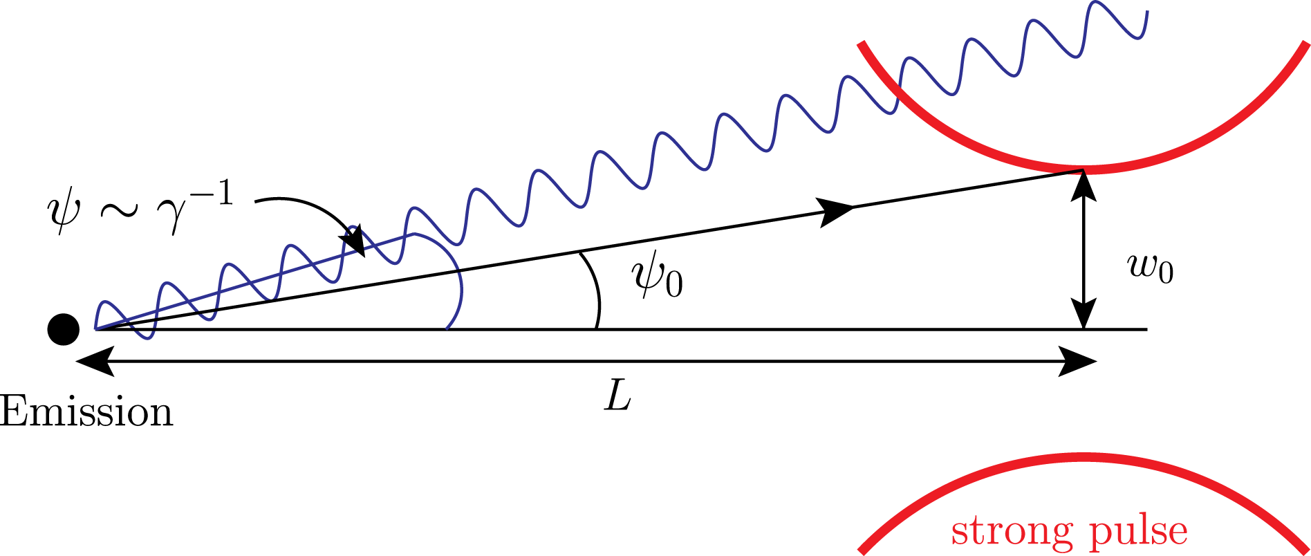
Figure 3. Sketch of experimental geometry, showing the distance between photon emission and interaction points. Emission is near forward,
 ${\it\psi}<1/{\it\gamma}$
, while the effective emission range of photons which can interact with the high-intensity pulse is limited to
${\it\psi}<1/{\it\gamma}$
, while the effective emission range of photons which can interact with the high-intensity pulse is limited to
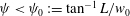 ${\it\psi}<{\it\psi}_{0}:=\tan ^{-1}L/w_{0}$
.
${\it\psi}<{\it\psi}_{0}:=\tan ^{-1}L/w_{0}$
.
Given a set-up as in figure 3 we can use (2.4) to calculate the flip probability
 $\mathbb{P}$
. Let
$\mathbb{P}$
. Let
 $\mathbb{P}_{0}$
be the ‘best case’ flip probability for photons arriving at the focal spot at the instant of peak field strength and with polarisation at
$\mathbb{P}_{0}$
be the ‘best case’ flip probability for photons arriving at the focal spot at the instant of peak field strength and with polarisation at
 $45^{\circ }$
to that of the intense optical pulse. Now consider deviations from the ideal case: the dependence of the probability on emission angle
$45^{\circ }$
to that of the intense optical pulse. Now consider deviations from the ideal case: the dependence of the probability on emission angle
 ${\it\psi}$
is easily guessed as being Gaussian, since the probability is expected to follow the intensity distribution squared. Indeed
${\it\psi}$
is easily guessed as being Gaussian, since the probability is expected to follow the intensity distribution squared. Indeed
 $$\begin{eqnarray}\mathbb{P}({\it\omega}^{\prime },{\it\psi})=\mathbb{P}_{0}({\it\omega}^{\prime })\text{e}^{-4{\it\psi}^{2}/{\it\psi}_{0}^{2}},\end{eqnarray}$$
gives a very good approximation of the flip probability: additional dependencies on geometric or polarisation angles due to perturbing away from the ideal case are effectively washed out by the very rapid falloff of the probability with
 ${\it\psi}$
. With this we can write down a simple model of the synchrotron emission spectrum following interaction with an intense pulse. Denoting the outgoing distribution with a prime, we write
${\it\psi}$
. With this we can write down a simple model of the synchrotron emission spectrum following interaction with an intense pulse. Denoting the outgoing distribution with a prime, we write
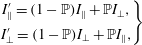 $$\begin{eqnarray}\left.\begin{array}{@{}c@{}}\displaystyle I_{\Vert }^{\prime }=(1-\mathbb{P})I_{\Vert }+\mathbb{P}I_{\bot },\\ \displaystyle I_{\bot }^{\prime }=(1-\mathbb{P})I_{\bot }+\mathbb{P}I_{\Vert },\end{array}\right\}\end{eqnarray}$$
(implying no photons are lost:
 $I^{\prime }:=I_{\Vert }^{\prime }+I_{\bot }^{\prime }=I$
). Vacuum polarisation then has a significant impact on the spectrum only for
$I^{\prime }:=I_{\Vert }^{\prime }+I_{\bot }^{\prime }=I$
). Vacuum polarisation then has a significant impact on the spectrum only for
 ${\it\psi}<{\it\psi}_{0}$
, as is illustrated in figure 2(b). With this model in hand we turn to quantitative estimates for a proposed experiment at ELI-NP (Nakamiya et al.
Reference Nakamiya, Homma, Moritaka and Seto2015).
${\it\psi}<{\it\psi}_{0}$
, as is illustrated in figure 2(b). With this model in hand we turn to quantitative estimates for a proposed experiment at ELI-NP (Nakamiya et al.
Reference Nakamiya, Homma, Moritaka and Seto2015).
4.1 Experiments at ELI-NP
The ELI proposal begins with the collision of highly relativistic electrons,
 ${\it\gamma}\gg 1$
, with a linearly polarised laser pulse. The electrons undergo Compton back scattering and emit instantaneously in a synchrotron spectrum (Jackson Reference Jackson1998). The polarisation direction of the emitted radiation is set by the plane of motion of the electrons, which is in turn set by the laser polarisation direction. The angle
${\it\gamma}\gg 1$
, with a linearly polarised laser pulse. The electrons undergo Compton back scattering and emit instantaneously in a synchrotron spectrum (Jackson Reference Jackson1998). The polarisation direction of the emitted radiation is set by the plane of motion of the electrons, which is in turn set by the laser polarisation direction. The angle
 ${\it\psi}$
, above, is the angle out of this plane.
${\it\psi}$
, above, is the angle out of this plane.
The produced high-energy photons are then used as the probe of a (second) laser pulse of very high intensity. The combination of high intensity and high energy increases the probability of helicity flip as the probe photons pass through the optical laser, see (2.4)–(2.5). After this interaction the polarisation of the high-energy photons is measured using a pair polarimeter (Nakamiya et al. Reference Nakamiya, Homma, Moritaka and Seto2015), see also below.
We assume generation of 2 GeV electrons which are collided with a laser pulse of, by modern standards, moderate intensity
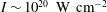 $I\sim 10^{20}~\text{W}~\text{cm}^{-2}$
. This generates radiation with a critical frequency of
$I\sim 10^{20}~\text{W}~\text{cm}^{-2}$
. This generates radiation with a critical frequency of
 ${\it\omega}_{c}=(3/2)m{\it\gamma}^{2}(E/E_{S})=0.24~\text{GeV}$
(using
${\it\omega}_{c}=(3/2)m{\it\gamma}^{2}(E/E_{S})=0.24~\text{GeV}$
(using
 $I=E^{2}/2$
) which is to interact with an intense optical pulse.
$I=E^{2}/2$
) which is to interact with an intense optical pulse.
We assume a distance of
 $L=20~\text{cm}$
between the emission point of the radiation and the interaction point with the intense pulse. Based on expected ELI parameters we take a focal radius
$L=20~\text{cm}$
between the emission point of the radiation and the interaction point with the intense pulse. Based on expected ELI parameters we take a focal radius
 $w_{0}=2.5~{\rm\mu}\text{m}$
. This gives the effective emission angle as
$w_{0}=2.5~{\rm\mu}\text{m}$
. This gives the effective emission angle as
 ${\it\psi}_{0}=\tan ^{-1}2.5~{\rm\mu}\text{m}/20~\text{cm}\simeq 10^{-5}$
, which is as suggested above much less than
${\it\psi}_{0}=\tan ^{-1}2.5~{\rm\mu}\text{m}/20~\text{cm}\simeq 10^{-5}$
, which is as suggested above much less than
 $1/{\it\gamma}\sim 3\times 10^{-4}$
. In order to write down the flip probability, we need the ‘best case’ result as described above (4.2). For a focussed Gaussian beam this has been found in Dinu et al. (Reference Dinu, Heinzl, Ilderton, Marklund and Torgrimsson2014a
) to be
$1/{\it\gamma}\sim 3\times 10^{-4}$
. In order to write down the flip probability, we need the ‘best case’ result as described above (4.2). For a focussed Gaussian beam this has been found in Dinu et al. (Reference Dinu, Heinzl, Ilderton, Marklund and Torgrimsson2014a
) to be
 $$\begin{eqnarray}\mathbb{P}_{0}({\it\omega}^{\prime })=\left(\frac{{\it\alpha}}{15}\frac{1}{E_{S}^{2}}\frac{{\mathcal{E}}{\it\omega}^{\prime }}{{\rm\pi}^{2}w_{0}^{2}}\right)^{2},\end{eqnarray}$$
where
 ${\mathcal{E}}$
is the energy of the laser. Based on expected ELI parameters we take
${\mathcal{E}}$
is the energy of the laser. Based on expected ELI parameters we take
 ${\mathcal{E}}=200\,\text{J}$
, which gives
${\mathcal{E}}=200\,\text{J}$
, which gives
 $$\begin{eqnarray}\mathbb{P}_{0}({\it\omega}^{\prime })\simeq 0.27\left(\frac{{\it\omega}^{\prime }}{\text{GeV}}\right)^{2}.\end{eqnarray}$$
This is significantly higher than for an optical X-ray set-up simply due to the higher probe energy (and the expected higher energies and intensities available at ELI). The flip probability as a function of
 ${\it\psi}$
is then given by (4.2).
${\it\psi}$
is then given by (4.2).
In the proposed experiment, the emitted radiation will be screened in order to ensure a high polarisation purity; only that part of the spectrum emitted at
 ${\it\psi}$
less than some small fraction, say 40 %, of
${\it\psi}$
less than some small fraction, say 40 %, of
 $1/{\it\gamma}$
will be allowed to propagate toward the high-intensity pulse (the target). A detector will be arranged to screen out (to some high degree) plane-polarised emission. The signal to be measured is then the increase in perpendicularly polarised photons incident on the detector due to vacuum polarisation effects. We can calculate the total energy deposited on the detector due to perpendicularly polarised photons fromFootnote
2
(Jackson Reference Jackson1998)
$1/{\it\gamma}$
will be allowed to propagate toward the high-intensity pulse (the target). A detector will be arranged to screen out (to some high degree) plane-polarised emission. The signal to be measured is then the increase in perpendicularly polarised photons incident on the detector due to vacuum polarisation effects. We can calculate the total energy deposited on the detector due to perpendicularly polarised photons fromFootnote
2
(Jackson Reference Jackson1998)
 $$\begin{eqnarray}\text{En}_{\bot }^{\prime }=\int _{0}^{0.4/{\it\gamma}}\,\text{d}{\it\psi}\int _{0}^{2\,\text{GeV}}\,\text{d}{\it\omega}^{\prime }I_{\bot }^{\prime }({\it\omega}^{\prime },{\it\psi})\simeq 1.16\text{En}_{\bot },\end{eqnarray}$$
which gives an increase of 16 %. A convenient measure of polarisation purity (which is also related to the polarimetry required to measure the photon polarisation in this set-up (Nakamiya et al. Reference Nakamiya, Homma, Moritaka and Seto2015)) is the ‘degree of linear polarisation’, which for the synchrotron spectrum before and after interaction with the intense laser pulse is defined by
 $$\begin{eqnarray}P_{lin}:=\frac{I_{\Vert }-I_{\bot }}{I_{\Vert }+I_{\bot }},\quad P_{lin}^{\prime }=\frac{I_{\Vert }^{\prime }-I_{\bot }^{\prime }}{I_{\Vert }^{\prime }+I_{\bot }^{\prime }}=(1-2\mathbb{P})P_{lin}.\end{eqnarray}$$
Vacuum polarisation effects will (for
 $\mathbb{P}<0.5$
) reduce the degree of linear polarisation: this is illustrated for the parameters considered here in figure 4.
$\mathbb{P}<0.5$
) reduce the degree of linear polarisation: this is illustrated for the parameters considered here in figure 4.
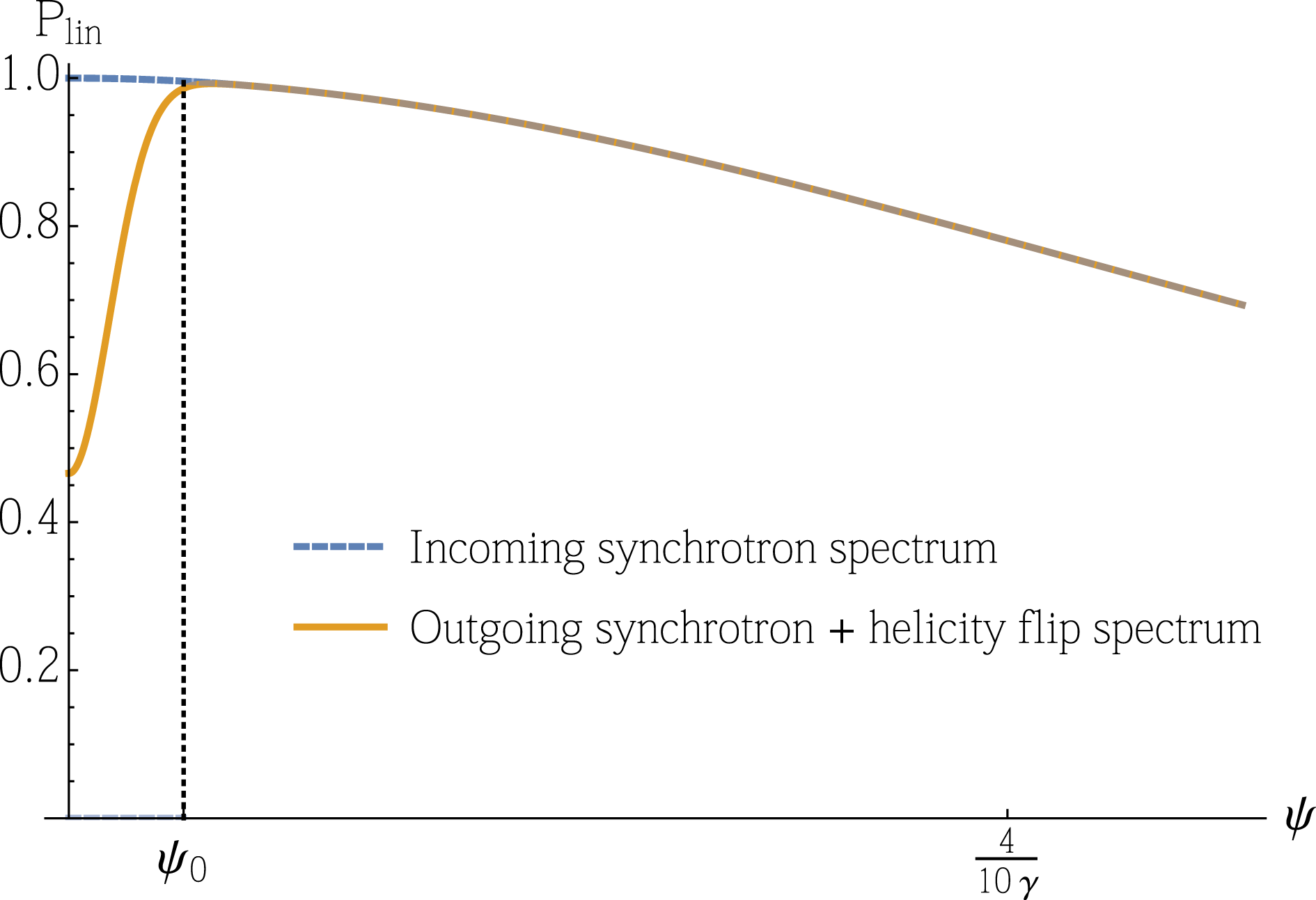
Figure 4. The degree of linear polarisation in the synchrotron spectrum (blue/dashed) and in the spectrum after passing through an intense field (yellow/solid) in which vacuum polarisation effects cause changes in photon polarisation. Plotted for 1 GeV probe photon energy and other parameters as in the text, for the proposed set-up at ELI-NP.
5 Discussion and conclusions
We have considered two proposals for measuring vacuum polarisation effects in strong laser fields. In the first, we used a dipole pulse as the ‘target’. The optimal focussing of dipole pulses yields high focal field strengths, which makes them ideal for studying pair creation (Gonoskov et al. Reference Gonoskov, Gonoskov, Harvey, Ilderton, Kim, Marklund, Mourou and Sergeev2013) and intense-field dynamics (Gonoskov et al. Reference Gonoskov, Bashinov, Gonoskov, Harvey, Ilderton, Kim, Marklund, Mourou and Sergeev2014). However the dipole pulse has a small (sub-wavelength) focal spot size, which can be disadvantageous for vacuum birefringence as the relevant observable there is sensitive to, essentially, the product of field strength and spot size.
The second method we have considered is the use of laser–particle collisions to generate high-energy gamma rays, which are in turn used as the probe of an intense optical pulse. We have provided a very simple ‘proof of principle’ calculation and seen that the high energy of the probe photons gives a large (ideal case) helicity-flip probability. The experimental realisation of the relevant set-up though will be challenging. Measurement of the signal requires pair polarimetry on the probe gamma rays; this is discussed in Nakamiya et al. (Reference Nakamiya, Homma, Moritaka and Seto2015). The use of a laser–particle collision to generate the probe in close proximity to the target suggests a ‘messy’ experimental environment. Only photons generated in a small volume of space, at the right time, will interact with the focal spot of the intense pulse and have an appreciable chance of changing helicity state; however the actual generation point can be anywhere in the volume of the laser–particle collision. This suggests that shot–shot fluctuations in signal and background may be large.
Refinements of the calculation presented here could begin with numerical simulations of the initial laser–particle interaction in order to better understand the spectrum of the generated probe photons (Elkina & King Reference Elkina and King2016). Here PIC methods would be useful, for a review of which, see Gonoskov et al. (Reference Gonoskov, Bastrakov, Efimenko, Ilderton, Marklund, Meyerov, Muraviev, Sergeev, Surmin and Wallin2015). (Polarisation effects would of course need to be included.) Once the spectrum is understood the impact of effects such as timing and pointing jitter can be included, and then a comprehensive picture of the background and signal sizes can be developed.
Acknowledgements
The authors are supported by the Olle Engkvist Foundation, grant 2014/744 (A.I.) and the Swedish Research Council, grants 2012-5644 and 2013-4248 (M.M.). A.I. thanks the coordinators of ELI-NP for the opportunity to join the facility’s Technical Design Report.


