


1. Introduction
Particle-based plasma simulations, including particle-in-cell (PIC) codes, are ubiquitous as a computational tool to understand plasma evolution, aiding research into nuclear fusion (Roth et al. Reference Roth, Cowan, Key, Hatchett, Brown, Fountain, Johnson, Pennington, Snavely and Wilks2001), proton radiography (Borghesi et al. Reference Borghesi, Sarri, Cecchetti, Kourakis, Hoarty, Stevenson, James, Brown, Hobbs and Lockyear2010) and hadron therapies (Bulanov & Khoroshkov Reference Bulanov and Khoroshkov2002). PIC codes with the ability to model particle–particle Coulomb collisions have become commonplace (Nanbu Reference Nanbu1997; Sentoku & Kemp Reference Sentoku and Kemp2008; Peano et al. Reference Peano, Marti, Silva and Coppa2009; Schmitz, Lloyd & Evans Reference Schmitz, Lloyd and Evans2012; Bobylev & Potapenko Reference Bobylev and Potapenko2013), and quantum electrodynamics is the latest area of physics that they have begun to include (Di Piazza et al. Reference Di Piazza, Müller, Hatsagortsyan and Keitel2012).
The addition of more physical phenomena means that increasingly complex interplays between different physics drives the overall evolution of plasmas in PIC simulations. In many applications of PIC, the objective is to understand the important processes behind an experimental result by running the simulations with similar conditions. Unravelling the exact interplay which causes particular effects to occur requires analysing the large amounts of particle-level data which are output by PIC simulations.
Here, we present a method to aid the analysis of the collisional interactions present in a PIC simulation. Usually, the collisional terms in the Boltzmann equation can only be evaluated from PIC output by integration over a six-dimensional phase space in each cell, which requires careful manipulation of often noisy distribution functions. These collisional terms are $Q_{s}$
and
$Q_{s}$
and $\boldsymbol{R}_{s}$
, which describe the exchange of energy density in time by species
$\boldsymbol{R}_{s}$
, which describe the exchange of energy density in time by species $s$
and the exchange of momentum density in time by species
$s$
and the exchange of momentum density in time by species $s$
, respectively. We provide a method to evaluate these terms using a simple sum over the properties of each particle in each cell. This simple sum can, in many case, be computed far more efficiently than the integration of the six-dimensional phase space.
$s$
, respectively. We provide a method to evaluate these terms using a simple sum over the properties of each particle in each cell. This simple sum can, in many case, be computed far more efficiently than the integration of the six-dimensional phase space.
This paper is organised as follows: § 2 sets out the advantages of this approach; § 3 defines the Boltzmann equation and its moments; § 4 states the main result of the work; § 5 contains the derivation of the results; and § 6 presents a computational benchmark of the results.
2. Merits of the approach
Evaluating the collisional terms $Q_{s}$
and
$Q_{s}$
and $\boldsymbol{R}_{s}$
defined in § 3 directly from distribution functions as output by PIC simulations requires two steps which can introduce errors. The first is in calculating continuous, smooth distribution functions from the properties of a discrete population of particles. This inevitably involves a binning procedure with a trade-off between resolving features in the distribution function and accepting noise in the value of
$\boldsymbol{R}_{s}$
defined in § 3 directly from distribution functions as output by PIC simulations requires two steps which can introduce errors. The first is in calculating continuous, smooth distribution functions from the properties of a discrete population of particles. This inevitably involves a binning procedure with a trade-off between resolving features in the distribution function and accepting noise in the value of $f_{s}$
as a function of
$f_{s}$
as a function of $\boldsymbol{v}$
. The proposed method requires no binning. The second involves performing the integration over the six-dimensional phase space. As a six-dimensional integration is a computationally intensive procedure, lower-order integration methods which admit more numerical error may be used. In the equations specified, only a direct sum over particle properties is required to evaluate
$\boldsymbol{v}$
. The proposed method requires no binning. The second involves performing the integration over the six-dimensional phase space. As a six-dimensional integration is a computationally intensive procedure, lower-order integration methods which admit more numerical error may be used. In the equations specified, only a direct sum over particle properties is required to evaluate $Q_{s}$
and
$Q_{s}$
and $\boldsymbol{R}_{s}$
.
$\boldsymbol{R}_{s}$
.
The extent of the computational advantage of directly evaluating the collisional terms, as opposed to performing the integration over phase space, depends upon the number of particles per cell and the binning procedure. A binning procedure with $B$
bins per momentum dimension for the particle distribution functions will require at least
$B$
bins per momentum dimension for the particle distribution functions will require at least $O(B^{6})$
computer operations in each cell for the evaluation of the collisional terms. In the equations described in § 4, evaluating the collision terms for
$O(B^{6})$
computer operations in each cell for the evaluation of the collisional terms. In the equations described in § 4, evaluating the collision terms for $N$
particles per cell requires
$N$
particles per cell requires $O(N^{2})$
computer operations. Given a typical
$O(N^{2})$
computer operations. Given a typical $B$
of 100, the direct evaluation method is more computationally efficient whenever
$B$
of 100, the direct evaluation method is more computationally efficient whenever $N<B^{3}\approx 10^{6}$
particles per cell.
$N<B^{3}\approx 10^{6}$
particles per cell.
The computations necessary to calculate $Q_{s}$
and
$Q_{s}$
and $\boldsymbol{R}_{s}$
could also be performed at run-time, as part of the operations of the base code. In this case, the energy and momentum transferred in each collision can be recorded in-line before and after each collision. However, widely used PIC codes do not already include this feature, and it would be an extraneous drain on computer and memory resources for simulations in which particle kinetics were not specifically of interest. Furthermore, most PIC modellers are end-users who may prefer not to modify the base code in this way. The proposed equations require only the output particle data with no modification of the base code; they can be used in post-processing. They also involve only a single evaluation per pair of particles (as opposed to a before and after evaluation for each particle-pair collision in-line).
$\boldsymbol{R}_{s}$
could also be performed at run-time, as part of the operations of the base code. In this case, the energy and momentum transferred in each collision can be recorded in-line before and after each collision. However, widely used PIC codes do not already include this feature, and it would be an extraneous drain on computer and memory resources for simulations in which particle kinetics were not specifically of interest. Furthermore, most PIC modellers are end-users who may prefer not to modify the base code in this way. The proposed equations require only the output particle data with no modification of the base code; they can be used in post-processing. They also involve only a single evaluation per pair of particles (as opposed to a before and after evaluation for each particle-pair collision in-line).
3. Boltzmann equation
The kinetic equation describing plasma evolution is the Boltzmann equation given by
 $$\begin{eqnarray}\frac{\partial f_{s}}{\partial t}+\frac{\partial }{\partial \boldsymbol{x}}\boldsymbol{\cdot }\boldsymbol{v}f_{s}+\frac{q_{s}}{m_{s}}\frac{\partial }{\partial \boldsymbol{v}}\boldsymbol{\cdot }(\boldsymbol{E}+\boldsymbol{v}\times \boldsymbol{B})f_{s}=C(f_{s}),\end{eqnarray}$$
where $f_{s}$
is the distribution of particles of species
$f_{s}$
is the distribution of particles of species $s$
defined by
$s$
defined by $n_{s}(\boldsymbol{x}_{s},t)=\int \,\text{d}^{3}v\,f_{s}(\boldsymbol{x}_{s},t,\boldsymbol{v}_{s})$
, with
$n_{s}(\boldsymbol{x}_{s},t)=\int \,\text{d}^{3}v\,f_{s}(\boldsymbol{x}_{s},t,\boldsymbol{v}_{s})$
, with $n_{s}$
the density of species
$n_{s}$
the density of species $s$
. Here
$s$
. Here $C(f_{s})=\sum _{s^{\prime }}C(f_{s},f_{s^{\prime }})$
is the collision operator. The labels
$C(f_{s})=\sum _{s^{\prime }}C(f_{s},f_{s^{\prime }})$
is the collision operator. The labels $s$
and
$s$
and $s^{\prime }$
refer to different species. Temperatures are expressed in units of energy throughout unless stated explicitly. Henceforth, Latin letters will refer to particles belonging to a particular species so that
$s^{\prime }$
refer to different species. Temperatures are expressed in units of energy throughout unless stated explicitly. Henceforth, Latin letters will refer to particles belonging to a particular species so that $i$
is a particle of species
$i$
is a particle of species $s$
and
$s$
and $j$
is a particle of species
$j$
is a particle of species $s^{\prime }$
. Greek letters refer to vector and matrix indices of rank three, i.e.
$s^{\prime }$
. Greek letters refer to vector and matrix indices of rank three, i.e. ${\bf\nu},{\bf\mu},$
etc., range over
${\bf\nu},{\bf\mu},$
etc., range over $1,2,3$
. In addition, bold font denotes a vector. Derivatives are denoted by
$1,2,3$
. In addition, bold font denotes a vector. Derivatives are denoted by
 $$\begin{eqnarray}\frac{\partial }{\partial v_{{\it\mu}}}\equiv \partial _{{\it\mu}},\quad \frac{\partial }{\partial v_{{\it\mu}}^{\prime }}\equiv \partial _{{\it\mu}}^{\prime },\end{eqnarray}$$
where primed and unprimed relate to species $s$
and
$s$
and $s^{\prime }$
respectively.
$s^{\prime }$
respectively.
We utilise the Landau collision operator, which is given by
 $$\begin{eqnarray}C(f_{s},f_{s^{\prime }})=-\partial _{{\it\nu}}\int \text{d}^{3}v^{\prime }\,Q_{{\it\nu}{\it\mu}}\left(\frac{\partial _{{\it\mu}}^{\prime }}{m_{s^{\prime }}}-\frac{\partial _{{\it\mu}}}{m_{s}}\right)f_{s}(\boldsymbol{v}_{s})f_{s^{\prime }}(\boldsymbol{v}_{s^{\prime }}),\end{eqnarray}$$
with collision kernel
 $$\begin{eqnarray}Q_{{\it\nu}{\it\mu}}={\it\chi}_{ss^{\prime }}U_{{\it\mu}{\it\nu}},\end{eqnarray}$$
where
 $$\begin{eqnarray}{\it\chi}_{ss^{\prime }}=\frac{2{\rm\pi}}{m_{s}}\ln {\it\Lambda}_{ss^{\prime }}\left(\frac{q_{s}q_{s^{\prime }}}{4{\rm\pi}{\it\epsilon}_{0}}\right)^{2}\end{eqnarray}$$
can be assumed to be constant including the Coulomb logarithm $\ln {\it\Lambda}$
, and
$\ln {\it\Lambda}$
, and
 $$\begin{eqnarray}U_{{\it\mu}{\it\nu}}=\left(\frac{u^{2}{\it\delta}_{{\it\mu}{\it\nu}}-u_{{\it\mu}}u_{{\it\nu}}}{u^{3}}\right).\end{eqnarray}$$
The relative velocity vector is given by $\boldsymbol{u}=\boldsymbol{v}-\boldsymbol{v}^{\prime }$
.
$\boldsymbol{u}=\boldsymbol{v}-\boldsymbol{v}^{\prime }$
.
The Landau collision operator is a small-angle collision-only approximation to the full Boltzmann collision operator, meaning that it is obtained by an expansion in ${\rm\Delta}\boldsymbol{v}$
and therefore ignores collisions with large scattering angles (Alexandre & Villani Reference Alexandre and Villani2004). However, the same approximation is used by most, if not all, PIC simulation collision algorithms, though methods to re-incorporate the collisions lost through this method are available (Turrell, Sherlock & Rose Reference Turrell, Sherlock and Rose2015). For most applications, ignoring large-angle collisions is valid because scattering via small angles is approximately
${\rm\Delta}\boldsymbol{v}$
and therefore ignores collisions with large scattering angles (Alexandre & Villani Reference Alexandre and Villani2004). However, the same approximation is used by most, if not all, PIC simulation collision algorithms, though methods to re-incorporate the collisions lost through this method are available (Turrell, Sherlock & Rose Reference Turrell, Sherlock and Rose2015). For most applications, ignoring large-angle collisions is valid because scattering via small angles is approximately $8\ln {\it\Lambda}$
more likely than via large angles.
$8\ln {\it\Lambda}$
more likely than via large angles.
The evolution of the plasma is described by the moments of the transport equation with the transport of energy given by the second moment,
 $$\begin{eqnarray}\displaystyle & & \displaystyle \frac{\partial }{\partial t}\left(\frac{3}{2}n_{s}T_{s}+\frac{1}{2}m_{s}n_{s}V_{s}^{2}\right)+\frac{\partial }{\partial \boldsymbol{x}}\boldsymbol{\cdot }\left[\boldsymbol{q}_{s}+\left(\frac{5}{2}n_{s}T_{s}+\frac{1}{2}n_{s}m_{s}V_{s}^{2}\right)\boldsymbol{V}_{s}+\boldsymbol{V}_{s}\boldsymbol{\cdot }{\it\bf\Pi}_{s}\right]\nonumber\\ \displaystyle & & \displaystyle \qquad -\,n_{s}q_{s}\boldsymbol{V}_{s}\boldsymbol{\cdot }\boldsymbol{E}-Q_{s}-\boldsymbol{V}_{s}\boldsymbol{\cdot }\boldsymbol{R}_{s}=0.\end{eqnarray}$$
The definition of these quantities is as follows, with $\boldsymbol{v}_{rel}=\boldsymbol{v}-\boldsymbol{V}_{s}$
and
$\boldsymbol{v}_{rel}=\boldsymbol{v}-\boldsymbol{V}_{s}$
and $\unicode[STIX]{x1D644}$
the identity matrix (also denoted by
$\unicode[STIX]{x1D644}$
the identity matrix (also denoted by ${\it\delta}_{{\it\mu}{\it\nu}}$
), and
${\it\delta}_{{\it\mu}{\it\nu}}$
), and $\boldsymbol{v},\boldsymbol{x},t$
dependence implicit:
$\boldsymbol{v},\boldsymbol{x},t$
dependence implicit:
 $$\begin{eqnarray}\displaystyle & \displaystyle \text{Drift velocity:}\quad \boldsymbol{V}_{s}\equiv \frac{1}{n_{s}}\int \,\text{d}^{3}v\,\boldsymbol{v}\,f_{s} & \displaystyle\end{eqnarray}$$
 $$\begin{eqnarray}\displaystyle & \displaystyle \text{Temperature:}\quad T_{s}\equiv \frac{1}{n_{s}}\int \,\text{d}^{3}v\frac{1}{3}m_{s}v_{rel}^{2}\,f_{s} & \displaystyle\end{eqnarray}$$
 $$\begin{eqnarray}\displaystyle & \displaystyle \text{Heat flux:}\quad \boldsymbol{q}_{s}\equiv \int \,\text{d}^{3}v\frac{1}{2}m_{s}v_{rel}^{2}\boldsymbol{v}_{rel}\,f_{s} & \displaystyle\end{eqnarray}$$
 $$\begin{eqnarray}\displaystyle & \displaystyle \text{Stress-tensor:}\quad {\it\bf\Pi}_{s}\equiv \int \,\text{d}^{3}v\,m_{s}\left(\boldsymbol{v}_{rel}\boldsymbol{v}_{rel}-\frac{1}{3}v_{rel}^{2}\unicode[STIX]{x1D644}\right)f_{s} & \displaystyle\end{eqnarray}$$
 $$\begin{eqnarray}\displaystyle & \displaystyle \text{Energy density rate:}\quad Q_{s}\equiv \int \,\text{d}^{3}v\frac{1}{2}m_{s}v_{rel}^{2}\mathop{\sum }_{s^{\prime }}C(f_{s},f_{s^{\prime }}) & \displaystyle\end{eqnarray}$$
 $$\begin{eqnarray}\displaystyle & \displaystyle \text{Momentum density rate:}\quad \boldsymbol{R}_{s}\equiv \int \,\text{d}^{3}v\,m_{s}\boldsymbol{v}\mathop{\sum }_{s^{\prime }}C(f_{s},f_{s^{\prime }}). & \displaystyle\end{eqnarray}$$
Note that $C(f_{s},f_{s^{\prime }})$
appears in the collisional energy exchange terms
$C(f_{s},f_{s^{\prime }})$
appears in the collisional energy exchange terms $\boldsymbol{R}_{s}$
and
$\boldsymbol{R}_{s}$
and $Q_{s}$
.
$Q_{s}$
.
PIC simulations explicitly keep track of particles’ positions and velocities so that within each grid cell a distribution function taking the form of a sum over delta functions may be defined for each species. Let this be
 $$\begin{eqnarray}f_{s}(\boldsymbol{x},\boldsymbol{v},t)=\frac{n_{s}(\boldsymbol{x},t)}{N_{s}}\mathop{\sum }_{i}{\it\delta}(\boldsymbol{v}-\boldsymbol{v}_{i})\end{eqnarray}$$
for $\boldsymbol{v}_{i}$
the velocity of the
$\boldsymbol{v}_{i}$
the velocity of the $i$
th particle of species
$i$
th particle of species $s$
,
$s$
, $N_{s}$
the total number of computational particles in the space and time element under consideration, and
$N_{s}$
the total number of computational particles in the space and time element under consideration, and ${\it\delta}(\boldsymbol{v})={\it\delta}(v_{x}){\it\delta}(v_{y}){\it\delta}(v_{z})$
.
${\it\delta}(\boldsymbol{v})={\it\delta}(v_{x}){\it\delta}(v_{y}){\it\delta}(v_{z})$
.
4. Results
The energy density exchange rate is given by
 $$\begin{eqnarray}Q_{s}=4{\rm\pi}\ln {\it\Lambda}_{ss^{\prime }}\frac{n_{s^{\prime }}n_{s}}{N_{s^{\prime }}N_{s}}\left(\frac{q_{s}q_{s^{\prime }}}{4{\rm\pi}{\it\epsilon}_{0}}\right)^{2}\mathop{\sum }_{i}\mathop{\sum }_{j}\frac{1}{u_{ij}^{3}}\left[\frac{u_{ij}^{2}}{m_{s}}-\frac{m_{s^{\prime }}+m_{s}}{m_{s^{\prime }}m_{s}}(\boldsymbol{v}_{i}-\boldsymbol{V}_{s})\boldsymbol{\cdot }\boldsymbol{u}_{ij}\right]\end{eqnarray}$$
and the momentum density exchange rate by
 $$\begin{eqnarray}\boldsymbol{R}_{s}=-4{\rm\pi}\ln {\it\Lambda}_{ss^{\prime }}\frac{n_{s^{\prime }}n_{s}}{N_{s^{\prime }}N_{s}}\left(\frac{q_{s}q_{s^{\prime }}}{4{\rm\pi}{\it\epsilon}_{0}}\right)^{2}\frac{m_{s^{\prime }}+m_{s}}{m_{s^{\prime }}m_{s}}\mathop{\sum }_{i}\mathop{\sum }_{j}\frac{\boldsymbol{u}_{ij}}{u_{ij}^{3}},\end{eqnarray}$$
where $\boldsymbol{u}_{ij}=\boldsymbol{v}_{i}-\boldsymbol{v}_{j}$
.
$\boldsymbol{u}_{ij}=\boldsymbol{v}_{i}-\boldsymbol{v}_{j}$
.
5. Derivation
The $i$
and
$i$
and $j$
labels will frequently be implicit in the derivation of the results. For Greek indices, the Einstein summation convention of summation over repeated indices is followed. It is assumed that the distribution functions are as defined in § 3. The following relations are useful,
$j$
labels will frequently be implicit in the derivation of the results. For Greek indices, the Einstein summation convention of summation over repeated indices is followed. It is assumed that the distribution functions are as defined in § 3. The following relations are useful,
 $$\begin{eqnarray}\partial _{{\it\mu}}U_{{\it\mu}{\it\nu}}=-2u_{{\it\nu}}/u^{3},\quad \partial _{{\it\mu}}^{\prime }U_{{\it\mu}{\it\nu}}=2u_{{\it\nu}}/u^{3},\end{eqnarray}$$
 $$\begin{eqnarray}\partial _{{\it\mu}}\left(\frac{2u_{{\it\mu}}}{u^{3}}\right)=0,\quad \partial _{{\it\mu}}^{\prime }\left(\frac{2u_{{\it\mu}}}{u^{3}}\right)=0.\end{eqnarray}$$
The collision operator is
 $$\begin{eqnarray}C(f_{s},f_{s^{\prime }})=-\partial _{{\it\nu}}\int \text{d}^{3}v^{\prime }{\it\chi}_{ss^{\prime }}U_{{\it\mu}{\it\nu}}\left(f_{s}\frac{\partial _{{\it\mu}}^{\prime }}{m_{s^{\prime }}}f_{s^{\prime }}-f_{s^{\prime }}\frac{\partial _{{\it\mu}}}{m_{s}}f_{s}\right)\end{eqnarray}$$
in which the second term, in $\partial _{{\it\mu}}f_{s}$
, may be trivially integrated to give
$\partial _{{\it\mu}}f_{s}$
, may be trivially integrated to give
 $$\begin{eqnarray}\partial _{{\it\nu}}\mathop{\sum }_{j}{\it\chi}_{ss^{\prime }}U_{{\it\mu}{\it\nu}}\frac{n_{s^{\prime }}}{N_{s^{\prime }}}\left(\frac{\partial _{{\it\mu}}}{m_{s}}f_{s}\right).\end{eqnarray}$$
Note that there is an implicit $i$
label on the matrix
$i$
label on the matrix $\unicode[STIX]{x1D650}$
. The first term, in
$\unicode[STIX]{x1D650}$
. The first term, in $\partial _{{\it\mu}}^{\prime }f_{s^{\prime }}$
, can be re-expressed as
$\partial _{{\it\mu}}^{\prime }f_{s^{\prime }}$
, can be re-expressed as
 $$\begin{eqnarray}\displaystyle -\!\partial _{{\it\nu}}\int \text{d}^{3}v^{\prime }\,{\it\chi}_{ss^{\prime }}U_{{\it\mu}{\it\nu}}\left(f_{s}\frac{\partial _{{\it\mu}}^{\prime }}{m_{s^{\prime }}}f_{s^{\prime }}\!\right)=-\partial _{{\it\nu}}\left\{\int _{{\it\Gamma}}\left[{\it\chi}_{ss^{\prime }}\hat{n}_{{\it\mu}}U_{{\it\mu}{\it\nu}}\frac{f_{s}\,f_{s^{\prime }}}{m_{s^{\prime }}}\right]\,\!\text{d}{\it\Gamma}-\!\int \text{d}^{3}v^{\prime }\,{\it\chi}_{ss^{\prime }}\frac{f_{s}\,f_{s^{\prime }}}{m_{s^{\prime }}}\partial _{{\it\mu}}^{\prime }U_{{\it\mu}{\it\nu}}\right\}\!, & & \displaystyle \nonumber\\ \displaystyle & & \displaystyle\end{eqnarray}$$
where $\hat{n}_{{\it\mu}}$
is the unit normal to the boundary,
$\hat{n}_{{\it\mu}}$
is the unit normal to the boundary, ${\it\Gamma}$
, of the velocity-space element
${\it\Gamma}$
, of the velocity-space element $\text{d}^{3}v$
. The boundary term vanishes to give
$\text{d}^{3}v$
. The boundary term vanishes to give
 $$\begin{eqnarray}\partial _{{\it\nu}}\mathop{\sum }_{j}\left({\it\chi}_{ss^{\prime }}\frac{n_{s^{\prime }}}{N_{s^{\prime }}}\frac{f_{s}}{m_{s^{\prime }}}2\frac{u_{{\it\nu}}}{u^{3}}\right),\end{eqnarray}$$
where the dependence of the relative velocity on $j$
is again implicit. Then
$j$
is again implicit. Then
 $$\begin{eqnarray}C(f_{s})=\mathop{\sum }_{j}{\it\chi}_{ss^{\prime }}\frac{n_{s^{\prime }}}{N_{s^{\prime }}}\partial _{{\it\nu}}\left(2\frac{f_{s}}{m_{s^{\prime }}}\frac{u_{{\it\nu}}}{u^{3}}+\frac{U_{{\it\mu}{\it\nu}}}{m_{s}}\partial _{{\it\mu}}\,f_{s}\right).\end{eqnarray}$$
The energy exchange rate density using this form of the collision operator is
 $$\begin{eqnarray}Q_{s}=\int \,\text{d}^{3}v\frac{1}{2}m_{s}v_{rel}^{2}\mathop{\sum }_{i}{\it\chi}_{ss^{\prime }}\frac{n_{s^{\prime }}}{N_{s^{\prime }}}\partial _{{\it\nu}}\left(2\frac{f_{s}}{m_{s^{\prime }}}\frac{u_{{\it\nu}}}{u^{3}}+\frac{U_{{\it\mu}{\it\nu}}}{m_{s}}\partial _{{\it\mu}}\,f_{s}\right)\!,\end{eqnarray}$$
which can be simplified to
 $$\begin{eqnarray}Q_{s}=-\frac{1}{2}m_{s}{\it\chi}_{ss^{\prime }}\frac{n_{s^{\prime }}}{N_{s^{\prime }}}\int \,\text{d}^{3}v\left(2\frac{f_{s}}{m_{s^{\prime }}}\frac{u_{{\it\nu}}}{u^{3}}+\frac{U_{{\it\mu}{\it\nu}}}{m_{s}}\partial _{{\it\mu}}\,f_{s}\right)2(v_{{\it\nu}}-V_{{\it\nu}}),\end{eqnarray}$$
where $V_{{\it\nu}}$
is the
$V_{{\it\nu}}$
is the ${\it\nu}$
th component of
${\it\nu}$
th component of $\boldsymbol{V}_{s}$
. Let the term in
$\boldsymbol{V}_{s}$
. Let the term in $U_{{\it\mu}{\it\nu}}$
be denoted by
$U_{{\it\mu}{\it\nu}}$
be denoted by $(\ast )$
so that
$(\ast )$
so that
 $$\begin{eqnarray}\displaystyle (\ast )=-\frac{1}{2}m_{s}{\it\chi}_{ss^{\prime }}\frac{n_{s^{\prime }}}{N_{s^{\prime }}}\left\{\int _{{\it\Gamma}}\left[\hat{n}_{{\it\mu}}2(v_{{\it\nu}}-V_{{\it\nu}})\frac{U_{{\it\mu}{\it\nu}}}{m_{s}}f_{s}\right]\,\text{d}{\it\Gamma}-\int \,\text{d}^{3}v\frac{2f_{s}}{m_{s}}\partial _{{\it\mu}}((v_{{\it\nu}}-V_{{\it\nu}})U_{{\it\mu}{\it\nu}})\right\} & & \displaystyle \nonumber\\ \displaystyle & & \displaystyle\end{eqnarray}$$
and so
 $$\begin{eqnarray}\displaystyle (\ast ) & = & \displaystyle {\it\chi}_{ss^{\prime }}\frac{n_{s^{\prime }}}{N_{s^{\prime }}}\int \,\text{d}^{3}v\,f_{s}[(v_{{\it\nu}}-V_{{\it\nu}})(-2u_{{\it\nu}}/u^{3})+U_{{\it\mu}{\it\mu}}]\nonumber\\ \displaystyle & = & \displaystyle {\it\chi}_{ss^{\prime }}\frac{n_{s^{\prime }}}{N_{s^{\prime }}}\int \,\text{d}^{3}v\frac{f_{s}}{u^{3}}[-2u_{{\it\nu}}(v_{{\it\nu}}-V_{{\it\nu}})+2u^{2}].\end{eqnarray}$$
The full expression is
 $$\begin{eqnarray}Q_{s}=\frac{1}{2}m_{s}{\it\chi}_{ss^{\prime }}\frac{n_{s^{\prime }}}{N_{s^{\prime }}}\int \,\text{d}^{3}v\frac{f_{s}}{u^{3}}\left[4\frac{u^{2}}{m_{s}}-4\frac{m_{s^{\prime }}+m_{s}}{m_{s^{\prime }}m_{s}}(v_{{\it\nu}}-V_{{\it\nu}})u_{{\it\nu}}\right].\end{eqnarray}$$
Evaluating the integral gives the result shown in § 4 for $Q_{s}$
.
$Q_{s}$
.
The momentum density rate is given by
 $$\begin{eqnarray}\displaystyle \boldsymbol{R}_{s} & = & \displaystyle \int \,\text{d}^{3}v\,m_{s}\boldsymbol{v}\mathop{\sum }_{j}{\it\chi}_{ss^{\prime }}\frac{n_{s^{\prime }}}{N_{s^{\prime }}}\partial _{{\it\nu}}\left(2\frac{f_{s}}{m_{s^{\prime }}}\frac{u_{{\it\nu}}}{u^{3}}+\frac{U_{{\it\mu}{\it\nu}}}{m_{s}}\partial _{{\it\mu}}\,f_{s}\right)\nonumber\\ \displaystyle & = & \displaystyle \mathop{\sum }_{j}m_{s}{\it\chi}_{ss^{\prime }}\frac{n_{s^{\prime }}}{N_{s^{\prime }}}\left\{\int _{{\it\Gamma}}\left[\boldsymbol{v}\hat{n}_{{\it\nu}}\left(2\frac{f_{s}}{m_{s^{\prime }}}\frac{u_{{\it\nu}}}{u^{3}}+\frac{U_{{\it\mu}{\it\nu}}}{m_{s}}\partial _{{\it\mu}}\,f_{s}\right)\right]\,\text{d}{\it\Gamma}\right.\nonumber\\ \displaystyle & & \displaystyle \left.-\,\int \,\text{d}^{3}v\left(2\frac{f_{s}}{m_{s^{\prime }}}\frac{u_{{\it\nu}}}{u^{3}}+\frac{U_{{\it\mu}{\it\nu}}}{m_{s}}\partial _{{\it\mu}}\,f_{s}\right)\partial _{{\it\nu}}\boldsymbol{v}\right\}.\end{eqnarray}$$
The ${\it\nu}$
th component of
${\it\nu}$
th component of $\boldsymbol{R}_{s}$
is then
$\boldsymbol{R}_{s}$
is then
 $$\begin{eqnarray}(R_{s})_{{\it\nu}}=-\int \,\text{d}^{3}v\mathop{\sum }_{j}m_{s}{\it\chi}_{ss^{\prime }}\frac{n_{s^{\prime }}}{N_{s^{\prime }}}\left[\left(2\frac{f_{s}}{m_{s^{\prime }}}\frac{u_{{\it\nu}}}{u^{3}}+\frac{U_{{\it\mu}{\it\nu}}}{m_{s}}\partial _{{\it\mu}}\,f_{s}\right)\right].\end{eqnarray}$$
The second term, in $U_{{\it\mu}{\it\nu}}$
, yields a contribution in the
$U_{{\it\mu}{\it\nu}}$
, yields a contribution in the ${\it\nu}$
th component of
${\it\nu}$
th component of
 $$\begin{eqnarray}\displaystyle & & \displaystyle -\mathop{\sum }_{j}m_{s}{\it\chi}_{ss^{\prime }}\frac{n_{s^{\prime }}}{N_{s^{\prime }}}\left\{\int _{{\it\Gamma}}\left[n_{{\it\mu}}\frac{U_{{\it\mu}{\it\nu}}}{m_{s}}f_{s}\right]\,\text{d}{\it\Gamma}-\int \,\text{d}^{3}v\,f_{s}\partial _{{\it\mu}}\frac{U_{{\it\mu}{\it\nu}}}{m_{s}}\right\}\nonumber\\ \displaystyle & & \displaystyle \quad =-\mathop{\sum }_{j}m_{s}{\it\chi}_{ss^{\prime }}\frac{n_{s^{\prime }}}{N_{s^{\prime }}}\int \,\text{d}^{3}v\,f_{s}\frac{2u_{{\it\nu}}}{m_{s}u^{3}},\end{eqnarray}$$
which leads to the result stated in § 4.
Note that the total energy transfer rate per unit volume due to collisions is given by
 $$\begin{eqnarray}\dot{{\it\epsilon}}_{s}=Q_{s}+\boldsymbol{R}_{s}\boldsymbol{\cdot }\boldsymbol{V}_{s},\end{eqnarray}$$
where the $s^{\prime }$
label is implicit, and that
$s^{\prime }$
label is implicit, and that
 $$\begin{eqnarray}\mathop{\sum }_{s^{\prime }}\dot{{\it\epsilon}}_{ss^{\prime }}=0.\end{eqnarray}$$
6. Benchmark
As a benchmark that the proposed equations give the correct values of the exchange rate densities, we evaluate the energy exchange density in a case for which there is a known analytical solution. The scenario is temperature equilibration between two species of ion with Maxwell–Boltzmann distributions,
 $$\begin{eqnarray}f_{s}(\boldsymbol{v})=n_{s}\left(\frac{m_{s}}{2{\rm\pi}T_{s}}\right)^{3/2}\exp \left[-\frac{m_{s}v^{2}}{2T_{s}}\right].\end{eqnarray}$$
The particle data used to evaluate $Q_{s}$
according to (4.1) is used to infer the rate of change of temperature of species
$Q_{s}$
according to (4.1) is used to infer the rate of change of temperature of species $s$
from
$s$
from
 $$\begin{eqnarray}\left(\frac{\text{d}T_{s}}{\text{d}t}\right)_{D}\equiv \frac{2}{3k_{B}n_{s}}Q_{s},\end{eqnarray}$$
where the above equation expresses temperature in units of degrees rather than in units of energy. The data used in (4.1) is taken from a particle Monte Carlo code which has been benchmarked for thermal equilibration problems (Turrell et al. Reference Turrell, Sherlock and Rose2015), and which uses Takizuka and Abe’s collision algorithm (Takizuka & Abe Reference Takizuka and Abe1977). Particles populate a single point but have three dimensions in velocity space, a situation sometimes abbreviated as ‘0D3V’, representing a single cell of a PIC simulation. Both species’ begin the simulation in equilibrium with themselves, but not with each other. This is compared with the Landau–Spitzer temperature equilibration rate for two Maxwell–Boltzmann distributions, which is given by (Spitzer Reference Spitzer1967)
 $$\begin{eqnarray}\left(\frac{\text{d}T_{s}}{\text{d}t}\right)_{LS}\equiv n_{s^{\prime }}\frac{8\sqrt{{\rm\pi}}}{3}\frac{\sqrt{2m_{s}}}{m_{s^{\prime }}}\left(\frac{q_{s}q_{s^{\prime }}}{4{\rm\pi}{\it\epsilon}_{0}}\right)^{2}\ln {\it\Lambda}_{ss^{\prime }}\left(T_{s}+\frac{m_{s}}{m_{s^{\prime }}}T_{s^{\prime }}\right)^{-3/2}(T_{s}-T_{s^{\prime }})\end{eqnarray}$$
in which $s\neq s^{\prime }$
and
$s\neq s^{\prime }$
and $T_{s}(t=0)\neq T_{s^{\prime }}(t=0)$
. The derivation of this equation is based on the Landau collision operator (Trubnikov Reference Trubnikov1965) in its equivalent formulation in terms of Rosenbluth potentials (Rosenbluth, MacDonald & Judd Reference Rosenbluth, MacDonald and Judd1957). For two ion species
$T_{s}(t=0)\neq T_{s^{\prime }}(t=0)$
. The derivation of this equation is based on the Landau collision operator (Trubnikov Reference Trubnikov1965) in its equivalent formulation in terms of Rosenbluth potentials (Rosenbluth, MacDonald & Judd Reference Rosenbluth, MacDonald and Judd1957). For two ion species $s$
and
$s$
and $s^{\prime }$
at a similar temperature and density, the temperature equilibration times are in the ratio
$s^{\prime }$
at a similar temperature and density, the temperature equilibration times are in the ratio
 $$\begin{eqnarray}\frac{{\it\tau}_{ss^{\prime }}}{{\it\tau}_{ss}}=\frac{m_{s^{\prime }}}{m_{s}}\left(\frac{m_{s^{\prime }}+m_{s}}{2m_{s^{\prime }}}\right)^{3/2}\end{eqnarray}$$
so that the intra-species equilibration time is shorter than the inter-species equilibration time regardless of the masses of the two species (Trubnikov Reference Trubnikov1965). Therefore, these species should maintain their own Maxwell–Boltzmann distributions during equilibration with each other.
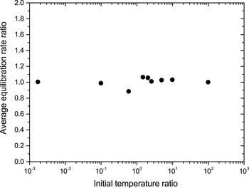
Figure 1. Results of 0D3V Monte Carlo simulations showing the equilibration rate ratio between Landau–Spitzer theory and (6.2) averaged over $5/{\it\nu}_{0}$
where
$5/{\it\nu}_{0}$
where ${\it\nu}_{0}$
is the initial equilibration frequency according to theory.
${\it\nu}_{0}$
is the initial equilibration frequency according to theory.
The results are shown in figure 1 and are expressed as the ratio of the Landau–Spitzer equilibration rate to the rate predicted by (6.2) as a function of the initial temperature ratio between the two ion species. There is excellent agreement between the theory and the computational estimate (which is also dependent on the resolution of the simulation) across a large range of temperature ratios.
Figure 1 provides a baseline scenario which uses $N=N_{s}=N_{s^{\prime }}=3333$
as the number of computational particles of each type of ion, and a computational time step of
$N=N_{s}=N_{s^{\prime }}=3333$
as the number of computational particles of each type of ion, and a computational time step of ${\rm\Delta}t={\it\tau}_{0}/10$
.
${\rm\Delta}t={\it\tau}_{0}/10$
. ${\it\tau}_{0}$
is
${\it\tau}_{0}$
is ${\it\tau}_{ss^{\prime }}(t=0)=1/{\it\nu}_{0}$
. To show the effects of varying
${\it\tau}_{ss^{\prime }}(t=0)=1/{\it\nu}_{0}$
. To show the effects of varying $N$
or
$N$
or ${\rm\Delta}t$
on the quality of the match with Landau–Spitzer theory, they are both varied relative to this base case. Figure 2 shows that the match is poorer with fewer computational particles as represented by the specific case of using
${\rm\Delta}t$
on the quality of the match with Landau–Spitzer theory, they are both varied relative to this base case. Figure 2 shows that the match is poorer with fewer computational particles as represented by the specific case of using $N/10$
. This is not a direct consequence of the equations shown in § 4 but a more general consequence of the reduction in accuracy when using fewer computational particles because, for example, the distribution functions of the ions will be more ‘noisy’, and less representative of the Maxwell–Boltzmann distribution assumed by the Landau–Spitzer theory. However, using
$N/10$
. This is not a direct consequence of the equations shown in § 4 but a more general consequence of the reduction in accuracy when using fewer computational particles because, for example, the distribution functions of the ions will be more ‘noisy’, and less representative of the Maxwell–Boltzmann distribution assumed by the Landau–Spitzer theory. However, using $10N$
computational particles demonstrates that the equations do converge on the Landau–Spitzer theory as the computational resolution is increased, and that the equations presented are accurate.
$10N$
computational particles demonstrates that the equations do converge on the Landau–Spitzer theory as the computational resolution is increased, and that the equations presented are accurate.

Figure 2. Results of 0D3V Monte Carlo simulations showing the equilibration rate ratio between Landau–Spitzer theory and (6.2) averaged over $5/{\it\nu}_{0}$
where
$5/{\it\nu}_{0}$
where ${\it\nu}_{0}$
for different numbers of computational particles.
${\it\nu}_{0}$
for different numbers of computational particles.
Similarly, figure 3 shows the effect of varying the computational time step, ${\rm\Delta}t$
. The results are less sensitive to this parameter as neither the Landau–Spitzer rate nor the equations in § 4 explicitly depend on the computational time step. However, there is an implicit dependence of the simulations: the (Takizuka & Abe Reference Takizuka and Abe1977) scattering routine used in the simulations relies on repeated small-angle collisions between computational particles with a scattering angle
${\rm\Delta}t$
. The results are less sensitive to this parameter as neither the Landau–Spitzer rate nor the equations in § 4 explicitly depend on the computational time step. However, there is an implicit dependence of the simulations: the (Takizuka & Abe Reference Takizuka and Abe1977) scattering routine used in the simulations relies on repeated small-angle collisions between computational particles with a scattering angle ${\it\theta}$
chosen from a distribution whose variance scales as
${\it\theta}$
chosen from a distribution whose variance scales as ${\rm\Delta}t$
. At large
${\rm\Delta}t$
. At large ${\rm\Delta}t$
, the scattering angles are no longer guaranteed to be small and the theory breaks down. Using
${\rm\Delta}t$
, the scattering angles are no longer guaranteed to be small and the theory breaks down. Using ${\rm\Delta}t\gg {\it\tau}/10$
would cause this to happen, and indirectly cause the results of evaluating (6.2) to become inaccurate. Figure 3 demonstrates that for
${\rm\Delta}t\gg {\it\tau}/10$
would cause this to happen, and indirectly cause the results of evaluating (6.2) to become inaccurate. Figure 3 demonstrates that for ${\rm\Delta}t={\it\tau}/10$
, varying
${\rm\Delta}t={\it\tau}/10$
, varying ${\rm\Delta}t$
by an order of magnitude largely maintains the accuracy of the equations in § 4.
${\rm\Delta}t$
by an order of magnitude largely maintains the accuracy of the equations in § 4.
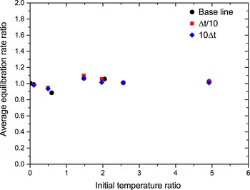
Figure 3. Results of 0D3V Monte Carlo simulations showing the equilibration rate ratio between Landau–Spitzer theory and (6.2) averaged over $5/{\it\nu}_{0}$
where
$5/{\it\nu}_{0}$
where ${\it\nu}_{0}$
for different computational time steps.
${\it\nu}_{0}$
for different computational time steps.
7. Conclusion
We have derived equations for plasma collisional energy exchange terms which are less computationally intensive to evaluate than the alternative methods available which use the output of PIC simulations. They involve a direct sum of the properties of particles rather than the integration of distribution functions over a six-dimensional velocity phase space. Results obtained using this method and data taken from particle simulations are in excellent agreement with the known test case problem of thermal equilibration, demonstrating that the derived equations are accurate.
Acknowledgements
A.E.T. was supported by EPSRC grants EP/L504786/1 and EP/K028464/1 while undertaking this research.


