


1. Introduction
In aeronautics, trailing vortices occur behind the wing of an aircraft due to the variation of the lift along the wing span. These vortices are characterized by strong axial velocity and relatively small wake deficit, which is recovered downstream due to the positive axial pressure gradient induced by the slowing down of the tangential motion caused by viscous effects. The analysis of their stability with respect to infinitesimal disturbances is important to better understand their lifetime as well as contrail formation. The tip vortices must be accounted for in the proper evaluation of aerodynamic loads and the induced drag, which represents approximately one third of the total drag of a civil aircraft. Its reduction, even by a small percentage, would correspond to a significant decrease in fuel consumption. Furthermore, the persistence of the trailing wake shed by an aircraft represents a source of risk for aircraft that follow in its wake, especially in takeoff and landing operations. For this reason, the minimum separation between aircraft in different operating conditions is prescribed by the International Civil Aviation Organization (ICAO).
Batchelor (Reference Batchelor1964) derived an asymptotic solution for trailing vortices by adopting boundary layer assumptions in incompressible axisymmetric Navier–Stokes equations, which rely on slow variation of the flow in the streamwise direction. This solution is commonly referred to as a Batchelor vortex, which in dimensional variables (
 $r^{\ast },x^{\ast }$
) reads
$r^{\ast },x^{\ast }$
) reads
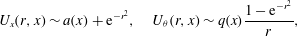
 $$\begin{eqnarray}\left.\begin{array}{@{}c@{}}\displaystyle U_{x}^{\ast }(r^{\ast },x^{\ast })\sim U_{\infty }+(U_{c}(x^{\ast })-U_{\infty })\text{e}^{-(r^{\ast }/R(x^{\ast }))^{2}},\\ \displaystyle U_{{\it\theta}}^{\ast }(r^{\ast },x^{\ast })\sim C_{0}\frac{1-\text{e}^{-(r^{\ast }/R(x^{\ast }))^{2}}}{r^{\ast }},\end{array}\right\}\end{eqnarray}$$
where
 $U_{x}^{\ast }$
and
$U_{x}^{\ast }$
and
 $U_{{\it\theta}}^{\ast }$
are the axial and azimuthal velocity components, and
$U_{{\it\theta}}^{\ast }$
are the axial and azimuthal velocity components, and
 $U_{\infty }$
is the free-stream velocity;
$U_{\infty }$
is the free-stream velocity;
 $U_{c}(x^{\ast })$
and
$U_{c}(x^{\ast })$
and
 $C_{0}$
are respectively the axial velocity at the centreline and the circulation divided by
$C_{0}$
are respectively the axial velocity at the centreline and the circulation divided by
 $2{\rm\pi}$
, and
$2{\rm\pi}$
, and
 $R(x^{\ast })$
is the vortex radius at the streamwise position
$R(x^{\ast })$
is the vortex radius at the streamwise position
 $x^{\ast }$
. For large Reynolds number,
$x^{\ast }$
. For large Reynolds number,
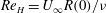
 $Re=U_{\infty }R(0)/{\it\nu}$
, the radial velocity
$Re=U_{\infty }R(0)/{\it\nu}$
, the radial velocity
 $U_{r}^{\ast }(r^{\ast },x^{\ast })\sim U_{\infty }/Re$
, which is negligible at leading order and results in a slow evolution of the flow in the streamwise direction. This allowed Batchelor (Reference Batchelor1964) to determine analytically the asymptotic streamwise evolution of
$U_{r}^{\ast }(r^{\ast },x^{\ast })\sim U_{\infty }/Re$
, which is negligible at leading order and results in a slow evolution of the flow in the streamwise direction. This allowed Batchelor (Reference Batchelor1964) to determine analytically the asymptotic streamwise evolution of
 $R(x^{\ast })$
and
$R(x^{\ast })$
and
 $U_{c}(x^{\ast })$
.
$U_{c}(x^{\ast })$
.
At a given downstream location, (1.1) can be made non-dimensional by choosing as length scale the radius core of the vortex,
 $R(x^{\ast })$
, and as velocity scale the velocity defect,
$R(x^{\ast })$
, and as velocity scale the velocity defect,
 ${\rm\Delta}U_{x}(x^{\ast })=U_{c}(x^{\ast })-U_{\infty }$
, see Delbende, Chomaz & Huerre (Reference Delbende, Chomaz and Huerre1998). Consequently, the so-called
${\rm\Delta}U_{x}(x^{\ast })=U_{c}(x^{\ast })-U_{\infty }$
, see Delbende, Chomaz & Huerre (Reference Delbende, Chomaz and Huerre1998). Consequently, the so-called
 $a{-}q$
formulation is obtained:
$a{-}q$
formulation is obtained:
 $$\begin{eqnarray}U_{x}(r,x)\sim a(x)+\text{e}^{-r^{2}},\quad U_{{\it\theta}}(r,x)\sim q(x)\frac{1-\text{e}^{-r^{2}}}{r},\end{eqnarray}$$
where
 $a\equiv U_{\infty }/{\rm\Delta}U$
is the external flow parameter,
$a\equiv U_{\infty }/{\rm\Delta}U$
is the external flow parameter,
 $q\equiv C_{0}/(R{\rm\Delta}U)$
is the swirl number and the local Reynolds number is defined as
$q\equiv C_{0}/(R{\rm\Delta}U)$
is the swirl number and the local Reynolds number is defined as
 $Re_{D}(x)=|{\rm\Delta}U(x)|R(x)/{\it\nu}$
. In contrast, if the free-stream velocity,
$Re_{D}(x)=|{\rm\Delta}U(x)|R(x)/{\it\nu}$
. In contrast, if the free-stream velocity,
 $U_{\infty }$
, and the initial vortex radius,
$U_{\infty }$
, and the initial vortex radius,
 $R(0)$
, are chosen as reference velocity and reference length, the following expressions are obtained, as in Heaton, Nichols & Schmid (Reference Heaton, Nichols and Schmid2009), which we will refer to as the
$R(0)$
, are chosen as reference velocity and reference length, the following expressions are obtained, as in Heaton, Nichols & Schmid (Reference Heaton, Nichols and Schmid2009), which we will refer to as the
 ${\it\alpha}{-}{\it\delta}$
formulation:
${\it\alpha}{-}{\it\delta}$
formulation:
 $$\begin{eqnarray}U_{x}(r,x)\sim 1-{\it\alpha}(x)\text{e}^{r^{2}/{\it\delta}^{2}(x)},\quad U_{{\it\theta}}(r,x)\sim k\frac{1-\text{e}^{-r^{2}/{\it\delta}^{2}(x)}}{r},\end{eqnarray}$$
where
 ${\it\alpha}$
is the non-dimensional wake defect
${\it\alpha}$
is the non-dimensional wake defect
 $-{\rm\Delta}U/U_{\infty }$
,
$-{\rm\Delta}U/U_{\infty }$
,
 $k$
is the non-dimensional circulation
$k$
is the non-dimensional circulation
 $k\equiv C_{0}/(R(0)U_{\infty })$
and
$k\equiv C_{0}/(R(0)U_{\infty })$
and
 ${\it\delta}(x)$
is the non-dimensional vortex radius
${\it\delta}(x)$
is the non-dimensional vortex radius
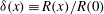 ${\it\delta}(x)\equiv R(x)/R(0)$
. Consequently, the local Reynolds number is defined as
${\it\delta}(x)\equiv R(x)/R(0)$
. Consequently, the local Reynolds number is defined as
 $Re_{H}=U_{\infty }R(0)/{\it\nu}$
. The relations among the quantities introduced in the two non-dimensionalizations are
$Re_{H}=U_{\infty }R(0)/{\it\nu}$
. The relations among the quantities introduced in the two non-dimensionalizations are
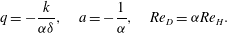 $$\begin{eqnarray}q=-\frac{k}{{\it\alpha}{\it\delta}},\quad a=-\frac{1}{{\it\alpha}},\quad Re_{D}={\it\alpha}Re_{H}.\end{eqnarray}$$
The parameters
 $a{-}q$
and
$a{-}q$
and
 ${\it\alpha}{-}{\it\delta}$
vary along the streamwise direction and mimic the vortex core spreading and the recovery of the wake deficit in the trailing-vortex evolution. By keeping these parameters constant the parallel Batchelor vortex is obtained, which is a family of columnar vortices identified by swirl number, wake deficit and Reynolds number.
${\it\alpha}{-}{\it\delta}$
vary along the streamwise direction and mimic the vortex core spreading and the recovery of the wake deficit in the trailing-vortex evolution. By keeping these parameters constant the parallel Batchelor vortex is obtained, which is a family of columnar vortices identified by swirl number, wake deficit and Reynolds number.
The linear stability of the parallel Batchelor vortex has been widely studied in the literature. Taken in isolation, the tangential velocity profile is stable, since it does not satisfy Rayleigh’s criterion, while the axial velocity profile is only unstable to mode
 $m=1$
(Batchelor & Gill Reference Batchelor and Gill1962) as a consequence of a shear instability. However, the addition of both velocity components leads to a massive destabilization for virtually any azimuthal mode when the swirl number is less than
$m=1$
(Batchelor & Gill Reference Batchelor and Gill1962) as a consequence of a shear instability. However, the addition of both velocity components leads to a massive destabilization for virtually any azimuthal mode when the swirl number is less than
 $q\approx 1.5$
(Leibovich & Stewartson Reference Leibovich and Stewartson1983; Mayer & Powell Reference Mayer and Powell1992; Delbende et al.
Reference Delbende, Chomaz and Huerre1998), the only cutoff mechanism being viscous damping. The mechanism underlying this destabilization is a generalized centrifugal instability unravelled by Ludwieg (Reference Ludwieg1962), Leibovich & Stewartson (Reference Leibovich and Stewartson1983) and Eckhoff (Reference Eckhoff1984). This general picture does not hold close to the stability bound
$q\approx 1.5$
(Leibovich & Stewartson Reference Leibovich and Stewartson1983; Mayer & Powell Reference Mayer and Powell1992; Delbende et al.
Reference Delbende, Chomaz and Huerre1998), the only cutoff mechanism being viscous damping. The mechanism underlying this destabilization is a generalized centrifugal instability unravelled by Ludwieg (Reference Ludwieg1962), Leibovich & Stewartson (Reference Leibovich and Stewartson1983) and Eckhoff (Reference Eckhoff1984). This general picture does not hold close to the stability bound
 $q=\sqrt{2}/2$
where weakly amplified modes have been detected. In addition, viscous core modes could also be identified numerically and asymptotically (Khorrami Reference Khorrami1991b
; Fabre & Jacquin Reference Fabre and Jacquin2004; Fabre, Sipp & Jacquin Reference Fabre, Sipp and Jacquin2006; Heaton Reference Heaton2007).
$q=\sqrt{2}/2$
where weakly amplified modes have been detected. In addition, viscous core modes could also be identified numerically and asymptotically (Khorrami Reference Khorrami1991b
; Fabre & Jacquin Reference Fabre and Jacquin2004; Fabre, Sipp & Jacquin Reference Fabre, Sipp and Jacquin2006; Heaton Reference Heaton2007).
Besides these temporal stability analyses, Delbende et al. (Reference Delbende, Chomaz and Huerre1998), Olendraru et al. (Reference Olendraru, Sellier, Rossi and Huerre1999) and Olendraru & Sellier (Reference Olendraru and Sellier2002) carried out a spatio-temporal analysis as a function of swirl and wake parameters, showing that for relatively large wake deficits the flow can be absolutely unstable, as seen in figure 2 of the present work. For coflowing wakes, the wake defect needed to trigger an absolute instability depends on the swirl number, and the lower bound is approximately
 $a=-1.25$
, corresponding of a wake deficit of 80 % of the external flow. Conversely, in the case of strong advection and moderate wake deficit, the flow is convectively unstable, with perturbations growing in space as they are simultaneously amplified and advected away. While Delbende et al. (Reference Delbende, Chomaz and Huerre1998) used the linear impulse response method, Olendraru et al. (Reference Olendraru, Sellier, Rossi and Huerre1999) and Olendraru & Sellier (Reference Olendraru and Sellier2002) used the pinch-point diagnostic for the transition from convective to absolute instability and carried out a spatial stability analysis computing the spatial growth rate as a function of the forcing frequency and the azimuthal wavenumber. In convectively unstable situations, they found that the helical symmetry of the most amplified mode changed drastically when spanning the forcing frequency,
$a=-1.25$
, corresponding of a wake deficit of 80 % of the external flow. Conversely, in the case of strong advection and moderate wake deficit, the flow is convectively unstable, with perturbations growing in space as they are simultaneously amplified and advected away. While Delbende et al. (Reference Delbende, Chomaz and Huerre1998) used the linear impulse response method, Olendraru et al. (Reference Olendraru, Sellier, Rossi and Huerre1999) and Olendraru & Sellier (Reference Olendraru and Sellier2002) used the pinch-point diagnostic for the transition from convective to absolute instability and carried out a spatial stability analysis computing the spatial growth rate as a function of the forcing frequency and the azimuthal wavenumber. In convectively unstable situations, they found that the helical symmetry of the most amplified mode changed drastically when spanning the forcing frequency,
 ${\it\omega}_{f}$
. This suggests that the mode selection in convectively unstable swirling flows strongly depends on the frequency spectrum of the incoming perturbations.
${\it\omega}_{f}$
. This suggests that the mode selection in convectively unstable swirling flows strongly depends on the frequency spectrum of the incoming perturbations.
Delbende & Rossi (Reference Delbende and Rossi2005) more recently also investigated the nonlinear response to the harmonic forcing of modes on an artificially maintained parallel swirling jet flow. They found that for low swirl (
 $q\leqslant 0.6$
), the flow saturates as an array of dipoles which cause an increase of the vortex core size. At intermediate values,
$q\leqslant 0.6$
), the flow saturates as an array of dipoles which cause an increase of the vortex core size. At intermediate values,
 $q\sim 0.8$
, the vortex breaks into an array of equal sign vortices, and for high swirl,
$q\sim 0.8$
, the vortex breaks into an array of equal sign vortices, and for high swirl,
 $q\geqslant 1$
, the increase of the instantaneous swirl induced by the accelerated diffusion of the axial core velocity favours flow relaminarization.
$q\geqslant 1$
, the increase of the instantaneous swirl induced by the accelerated diffusion of the axial core velocity favours flow relaminarization.
Although these results strictly apply for the parallel Batchelor vortex, they are of fundamental importance for real non-parallel flows, because it is known that the global stability features are related to the local stability properties, see Huerre & Monkewitz (Reference Huerre and Monkewitz1990) and Chomaz (Reference Chomaz2005) for a comprehensive discussion. In the non-parallel framework, Heaton et al. (Reference Heaton, Nichols and Schmid2009) carried out a global analysis, considering the baseflow resulting from the imposition of a 90 % wake deficit at the inlet, i.e.
 ${\it\alpha}(0)=0.9$
. As the wake deficit is progressively recovered downstream, the flow turns convectively unstable, but for the chosen inlet parameters and Reynolds number, the flow exhibits a sufficiently extended absolutely unstable region to become globally unstable. The frequency of the most unstable global mode is indeed observed to match the absolute frequency prevailing at the inlet, as long as the domain is short enough for an accurate resolution of the resulting eigenvalue problem. However, typical trailing vortices have a rather strong axial velocity component, as experimentally measured by Devenport et al. (Reference Devenport, Rife, Liapis and Follin1996) and more recently by del Pino et al. (Reference del Pino, Parras, Felli and Fernandez-Feria2011), with wake deficits typically less than 80 %. These flows are locally convectively unstable everywhere and behave as noise amplifiers. In this work the mode selection in a harmonically forced non-parallel Batchelor vortex is considered, and the capability to predict the amplitude and spatial shape of the response by linear analyses is investigated.
${\it\alpha}(0)=0.9$
. As the wake deficit is progressively recovered downstream, the flow turns convectively unstable, but for the chosen inlet parameters and Reynolds number, the flow exhibits a sufficiently extended absolutely unstable region to become globally unstable. The frequency of the most unstable global mode is indeed observed to match the absolute frequency prevailing at the inlet, as long as the domain is short enough for an accurate resolution of the resulting eigenvalue problem. However, typical trailing vortices have a rather strong axial velocity component, as experimentally measured by Devenport et al. (Reference Devenport, Rife, Liapis and Follin1996) and more recently by del Pino et al. (Reference del Pino, Parras, Felli and Fernandez-Feria2011), with wake deficits typically less than 80 %. These flows are locally convectively unstable everywhere and behave as noise amplifiers. In this work the mode selection in a harmonically forced non-parallel Batchelor vortex is considered, and the capability to predict the amplitude and spatial shape of the response by linear analyses is investigated.
The objective of this work is to analyse the mode selection in a non-parallel spatially evolving Batchelor vortex subjected to harmonic in time but random in space perturbations. After the introduction of the prototype trailing vortex used throughout the work in § 2, the observation of the nonlinear response to a harmonic inlet forcing computed by three-dimensional (3D) direct numerical simulation (DNS) is briefly reported in § 3. In § 4, the linear flow response to boundary forcing is investigated using the WKB (Wentzel, Kramers, Brillouin) asymptotic analysis in the framework of weakly non-parallel flow. The asymptotic results are then compared with the results of a global analysis, which relaxes the weakly non-parallel assumption. The optimal inlet forcing, which maximizes the linear energy amplification of the response, is thus determined through a global resolvent. In § 5 the flow response to a volume forcing is computed using both the global resolvent approach and a generalized WKB analysis. The effect of nonlinearity on the response is investigated in § 6 in the case of inlet forcing. The nonlinear gains are computed through DNS as a function of the forcing frequency and for increasing forcing amplitudes. The mode selection observed in the DNS is compared with the one of the linear optimal response. Finally, conclusions are outlined.
Several sets of equations, all derived from Navier–Stokes equations, are used in this study to conduct the different steps of the analysis, which all require adequate numerical methods. We have chosen to describe these methods briefly when the corresponding equations are progressively introduced.
2. Trailing-vortex prototype
In the present work a typical trailing vortex is considered and used as the test case. This prototype flow with velocity
 $\boldsymbol{U}_{b}$
and pressure
$\boldsymbol{U}_{b}$
and pressure
 $P_{b}$
satisfies the steady axisymmetric Navier–Stokes equations
$P_{b}$
satisfies the steady axisymmetric Navier–Stokes equations
 $$\begin{eqnarray}\left.\begin{array}{@{}c@{}}\displaystyle \boldsymbol{U}_{b}\boldsymbol{\cdot }\boldsymbol{{\rm\nabla}}\boldsymbol{U}_{b}=-\boldsymbol{{\rm\nabla}}P_{b}+\frac{1}{Re}{\rm\Delta}\boldsymbol{U}_{b},\\ \displaystyle \boldsymbol{{\rm\nabla}}\boldsymbol{\cdot }\boldsymbol{ U}_{b}=0,\\ \displaystyle \boldsymbol{ U}_{b}=\boldsymbol{U}_{0}\quad \text{on}~{\it\Gamma}_{i}.\end{array}\right\}\end{eqnarray}$$
A parallel Batchelor profile,
 $\boldsymbol{U}_{0}$
, in the
$\boldsymbol{U}_{0}$
, in the
 ${\it\alpha},{\it\delta}$
formulation is imposed at the inlet,
${\it\alpha},{\it\delta}$
formulation is imposed at the inlet,
 ${\it\Gamma}_{i}$
, as a Dirichlet boundary condition with
${\it\Gamma}_{i}$
, as a Dirichlet boundary condition with
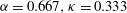 ${\it\alpha}=0.667,{\it\kappa}=0.333$
. A free-stress boundary condition is imposed at the outlet,
${\it\alpha}=0.667,{\it\kappa}=0.333$
. A free-stress boundary condition is imposed at the outlet,
 ${\it\Gamma}_{o}$
, and lateral boundary,
${\it\Gamma}_{o}$
, and lateral boundary,
 ${\it\Gamma}_{l}$
, while symmetry conditions are imposed on the axis. The Reynolds number is defined using as reference length the size of the vortex core at the inlet and is equal to
${\it\Gamma}_{l}$
, while symmetry conditions are imposed on the axis. The Reynolds number is defined using as reference length the size of the vortex core at the inlet and is equal to
 $Re_{H}=1000$
(
$Re_{H}=1000$
(
 $Re_{D}=667$
). Taking advantage of the local stability of Batchelor vortices with respect to
$Re_{D}=667$
). Taking advantage of the local stability of Batchelor vortices with respect to
 $m=0$
axisymmetric perturbations, this steady solution is obtained by time-marching an axisymmetric simulation with the spectral element code Nek5000 (Fischer, James & Kerkemeier Reference Fischer, James and Kerkemeier2008). The flow is considered steady when the
$m=0$
axisymmetric perturbations, this steady solution is obtained by time-marching an axisymmetric simulation with the spectral element code Nek5000 (Fischer, James & Kerkemeier Reference Fischer, James and Kerkemeier2008). The flow is considered steady when the
 $L^{2}$
-norm of the difference between two consecutive solutions is less than
$L^{2}$
-norm of the difference between two consecutive solutions is less than
 $10^{-12}$
. The computational domain is
$10^{-12}$
. The computational domain is
 $0\leqslant x\leqslant 40$
and
$0\leqslant x\leqslant 40$
and
 $0\leqslant r\leqslant 10$
(see appendix C for discussion of the influence of the radial extension of the domain). The resulting steady flow,
$0\leqslant r\leqslant 10$
(see appendix C for discussion of the influence of the radial extension of the domain). The resulting steady flow,
 $\boldsymbol{U}_{b}$
, is reported in figure 1 as (a,b) axial, (c,d) azimuthal and (e,f) radial velocity components, showing the gradual recovery of the wake deficit, as one proceeds downstream, and the diffusion of the vortical core. The radial velocity is significantly smaller than the other two velocity components, thus validating the boundary layer assumptions adopted by Batchelor. This is due to the fact that the streamwise evolution of a trailing vortex is governed by viscous effects, which operate at a slower time scale with respect to advection. The present flow can be qualified as weakly non-parallel, meaning that at first order the flow field
$\boldsymbol{U}_{b}$
, is reported in figure 1 as (a,b) axial, (c,d) azimuthal and (e,f) radial velocity components, showing the gradual recovery of the wake deficit, as one proceeds downstream, and the diffusion of the vortical core. The radial velocity is significantly smaller than the other two velocity components, thus validating the boundary layer assumptions adopted by Batchelor. This is due to the fact that the streamwise evolution of a trailing vortex is governed by viscous effects, which operate at a slower time scale with respect to advection. The present flow can be qualified as weakly non-parallel, meaning that at first order the flow field
 $\boldsymbol{U}(x,r)$
can be seen as a sequence of parallel Batchelor vortices. Hence, the streamwise evolution of the trailing vortex can be represented as a path in the
$\boldsymbol{U}(x,r)$
can be seen as a sequence of parallel Batchelor vortices. Hence, the streamwise evolution of the trailing vortex can be represented as a path in the
 $(a,q)$
plane, starting at
$(a,q)$
plane, starting at
 $a=-1.5$
and
$a=-1.5$
and
 $q=-0.5$
, see figure 2.
$q=-0.5$
, see figure 2.

Figure 1. (a,b) Streamwise, (c,d) azimuthal and (e,f) radial velocity components of the axisymmetric Navier–Stokes steady solution obtained by setting at the inlet a parallel Batchelor profile with
 ${\it\alpha}(0)=0.667,{\it\kappa}(0)=0.333$
, which is depicted in (a,c,e).
${\it\alpha}(0)=0.667,{\it\kappa}(0)=0.333$
, which is depicted in (a,c,e).
The present choice of prototype trailing vortex has been motivated by the fact that for higher or lower swirl numbers the flow is close to neutral stability conditions and perturbations are less amplified. With this choice of negative but large-amplitude advection parameter at the inlet, the locus of the local baseflow characteristic parameters in the
 $(a,q)$
plane does not penetrate into the absolutely unstable region. This flow is therefore globally stable and behaves as a noise amplifier. The stability of the baseflow has been checked numerically using the discretization method discussed in § 4, and the least stable eigenvalue is found to be
$(a,q)$
plane does not penetrate into the absolutely unstable region. This flow is therefore globally stable and behaves as a noise amplifier. The stability of the baseflow has been checked numerically using the discretization method discussed in § 4, and the least stable eigenvalue is found to be
 ${\it\omega}=0.5609-0.202\text{i}$
, corresponding to the azimuthal wavenumber
${\it\omega}=0.5609-0.202\text{i}$
, corresponding to the azimuthal wavenumber
 $m=1$
. As a comparison, the dotted path intersecting the region of absolute instability in figure 2 corresponds to the globally unstable non-parallel swirling flow considered by Heaton et al. (Reference Heaton, Nichols and Schmid2009).
$m=1$
. As a comparison, the dotted path intersecting the region of absolute instability in figure 2 corresponds to the globally unstable non-parallel swirling flow considered by Heaton et al. (Reference Heaton, Nichols and Schmid2009).

Figure 2. Figure adapted from Delbende et al. (Reference Delbende, Chomaz and Huerre1998). The regions of absolute (AI) and convective (CI) instability are reported in the
 $(a,q)$
parameter space for the Reynolds number
$(a,q)$
parameter space for the Reynolds number
 $Re_{D}=667$
. The path shown by the solid line depicts the local properties of the non-parallel trailing vortex studied in this work. The dashed line identifies the globally unstable non-parallel Batchelor vortex investigated in Heaton et al. (Reference Heaton, Nichols and Schmid2009).
$Re_{D}=667$
. The path shown by the solid line depicts the local properties of the non-parallel trailing vortex studied in this work. The dashed line identifies the globally unstable non-parallel Batchelor vortex investigated in Heaton et al. (Reference Heaton, Nichols and Schmid2009).
3. Observation of the nonlinear response to harmonic inlet forcing
In this section the nonlinear response of a trailing vortex to a harmonic forcing is investigated by full 3D DNS. Specifically, a harmonic inlet forcing acting on the three velocity components has been considered. The forcing adopted is chosen random in space in order to better enlighten the role of the forcing frequency on the change of the structure of the response.
The unsteady Navier–Stokes equations
 $$\begin{eqnarray}\left.\begin{array}{@{}c@{}}\displaystyle \frac{\partial \boldsymbol{U}}{\partial t}+\boldsymbol{U}\boldsymbol{\cdot }\boldsymbol{{\rm\nabla}}\displaystyle \boldsymbol{U}=-\boldsymbol{{\rm\nabla}}P+\frac{1}{Re}{\rm\Delta}\boldsymbol{U},\\ \displaystyle \boldsymbol{{\rm\nabla}}\boldsymbol{\cdot }\boldsymbol{ U}=0\end{array}\right\}\end{eqnarray}$$
are solved in a cylindrical domain of radius
 $r_{max}=10$
and length
$r_{max}=10$
and length
 $x_{max}=40$
, complemented with free-stress boundary conditions on all domain boundaries except at the inlet
$x_{max}=40$
, complemented with free-stress boundary conditions on all domain boundaries except at the inlet
 ${\it\Gamma}_{i}$
, where an unsteady Dirichlet boundary condition fluctuating around the baseflow inlet profile is imposed,
${\it\Gamma}_{i}$
, where an unsteady Dirichlet boundary condition fluctuating around the baseflow inlet profile is imposed,
 $$\begin{eqnarray}\boldsymbol{U}=\boldsymbol{U}_{0}+a_{{\it\zeta}}{\bf\zeta}\cos ({\it\omega}_{f}t)\quad \text{on}~{\it\Gamma}_{i}.\end{eqnarray}$$
A random inlet field concentrated in the region
 $r\leqslant 5$
is generated offline before the first time step and saved in memory invoking the MATLAB function rand which returns pseudorandom numbers uniformly distributed between 0 and 1. These fields are then loaded in Nek5000 and projected in the space of continuous functions, obtaining the fields
$r\leqslant 5$
is generated offline before the first time step and saved in memory invoking the MATLAB function rand which returns pseudorandom numbers uniformly distributed between 0 and 1. These fields are then loaded in Nek5000 and projected in the space of continuous functions, obtaining the fields
 ${\bf\zeta}=({\it\zeta}_{x}(y,z),{\it\zeta}_{y}(y,z),{\it\zeta}_{z}(y,z))$
. Three forcing amplitudes have been considered,
${\bf\zeta}=({\it\zeta}_{x}(y,z),{\it\zeta}_{y}(y,z),{\it\zeta}_{z}(y,z))$
. Three forcing amplitudes have been considered,
 $a_{{\it\zeta}}=0.01,~0.05$
and 0.1. The Navier–Stokes equations are solved in Cartesian coordinates using the Nek5000 spectral elements solver, while the time discretization is ensured using a Crank–Nicolson scheme. Convergence is attained with 2.2 million degrees of freedom and the code is parallelized. The integration time was equal is 400 time units, sufficiently large to capture the flow dynamics of the permanent regime. The time evolution of the energy of the flow was used to assess that a periodic permanent regime was indeed reached.
$a_{{\it\zeta}}=0.01,~0.05$
and 0.1. The Navier–Stokes equations are solved in Cartesian coordinates using the Nek5000 spectral elements solver, while the time discretization is ensured using a Crank–Nicolson scheme. Convergence is attained with 2.2 million degrees of freedom and the code is parallelized. The integration time was equal is 400 time units, sufficiently large to capture the flow dynamics of the permanent regime. The time evolution of the energy of the flow was used to assess that a periodic permanent regime was indeed reached.
The forcing frequency
 ${\it\omega}_{f}$
ranges from 0.1 to 5 and the spatial structure of the response is monitored by observing its azimuthal symmetries. Figure 3 reports isosurfaces of axial vorticity at the streamwise section
${\it\omega}_{f}$
ranges from 0.1 to 5 and the spatial structure of the response is monitored by observing its azimuthal symmetries. Figure 3 reports isosurfaces of axial vorticity at the streamwise section
 $x=30$
for different values of the forcing frequency. At low frequency, low azimuthal wavenumbers are the most amplified, while at higher frequency, higher wavenumbers are excited by the forcing. For instance, at frequency
$x=30$
for different values of the forcing frequency. At low frequency, low azimuthal wavenumbers are the most amplified, while at higher frequency, higher wavenumbers are excited by the forcing. For instance, at frequency
 ${\it\omega}_{f}=0.50$
, a single spiral mode is excited, while for
${\it\omega}_{f}=0.50$
, a single spiral mode is excited, while for
 ${\it\omega}_{f}=1.00$
the response is dominated by a double-helical structure. On increasing the forcing frequency further, triple (
${\it\omega}_{f}=1.00$
the response is dominated by a double-helical structure. On increasing the forcing frequency further, triple (
 ${\it\omega}_{f}=1.80$
), quadruple (
${\it\omega}_{f}=1.80$
), quadruple (
 ${\it\omega}_{f}=2.40$
) or higher helical structures appear. In this swirling flow, the spatial shape of the response is found to be very sensitive to the forcing frequency, calling for a detailed understanding of the mode-selection mechanism.
${\it\omega}_{f}=2.40$
) or higher helical structures appear. In this swirling flow, the spatial shape of the response is found to be very sensitive to the forcing frequency, calling for a detailed understanding of the mode-selection mechanism.

Figure 3. Isocontours of the axial vorticity at the streamwise section
 $x=30$
for different forcing frequencies. The amplitude of the forcing was set equal to
$x=30$
for different forcing frequencies. The amplitude of the forcing was set equal to
 $a_{{\it\zeta}}=0.01$
.
$a_{{\it\zeta}}=0.01$
.
4. Linear response to harmonic inlet forcing
In a parallel convectively unstable flow, the spatial stability branches fully describe the response to a harmonic forcing at any point of the domain, see Huerre & Rossi (Reference Huerre and Rossi1998). The spatial analysis provides the amplification in space,
 $-k_{i}$
, and the axial wavenumber,
$-k_{i}$
, and the axial wavenumber,
 $k_{r}$
, of a downstream propagating perturbation with frequency
$k_{r}$
, of a downstream propagating perturbation with frequency
 ${\it\omega}_{f}$
. In this framework
${\it\omega}_{f}$
. In this framework
 $k$
is the complex eigenvalue of the polynomial eigenvalue problem obtained from the linearized stability equations after the introduction of a normal mode expansion
$k$
is the complex eigenvalue of the polynomial eigenvalue problem obtained from the linearized stability equations after the introduction of a normal mode expansion
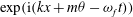 $\exp (\text{i}(kx+m{\it\theta}-{\it\omega}_{f}t))$
. Following Iungo et al. (Reference Iungo, Viola, Camarri and Gallaire2013), the corresponding stability equations in primitive variables around a parallel baseflow
$\exp (\text{i}(kx+m{\it\theta}-{\it\omega}_{f}t))$
. Following Iungo et al. (Reference Iungo, Viola, Camarri and Gallaire2013), the corresponding stability equations in primitive variables around a parallel baseflow
 $U_{{\it\theta}}(r),U_{x}(r)$
are
$U_{{\it\theta}}(r),U_{x}(r)$
are
 $$\begin{eqnarray}\left.\begin{array}{@{}c@{}}\displaystyle -\text{i}{\it\omega}_{f}u_{r}+{\it\Gamma}_{m,k}u_{r}-2{\it\Omega}u_{{\it\theta}}=-\frac{\partial p}{\partial r}+\frac{1}{Re}\left[\left({\it\Delta}_{m,k}-\frac{1}{r^{2}}\right)u_{r}-\frac{2\text{i}mu_{{\it\theta}}}{r^{2}}\right],\\ \displaystyle -\text{i}{\it\omega}_{f}u_{{\it\theta}}+{\it\Gamma}_{m,k}u_{{\it\theta}}+u_{r}\frac{\partial U_{{\it\theta}}}{\partial r}+{\it\Omega}u_{r}=-\frac{\text{i}mp}{r}+\frac{1}{Re}\left[\left({\it\Delta}_{m,k}-\frac{1}{r^{2}}\right)u_{{\it\theta}}+\frac{2\text{i}mu_{r}}{r^{2}}\right],\\ \displaystyle -\text{i}{\it\omega}_{f}u_{x}+{\it\Gamma}_{m,k}u_{x}+u_{r}\frac{\partial U_{x}}{\partial r}=-\text{i}kp+\frac{1}{Re}{\it\Delta}_{m,k}u_{x},\\ \displaystyle \frac{1}{r}\frac{\partial (ru_{r})}{\partial r}+\frac{\text{i}mu_{{\it\theta}}}{r}+\text{i}ku_{x}=0,\end{array}\right\}\end{eqnarray}$$
where
 ${\it\Omega}=U_{{\it\theta}}/r$
,
${\it\Omega}=U_{{\it\theta}}/r$
,
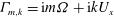 ${\it\Gamma}_{m,k}=\text{i}m{\it\Omega}+\text{i}kU_{x}$
and
${\it\Gamma}_{m,k}=\text{i}m{\it\Omega}+\text{i}kU_{x}$
and
 ${\it\Delta}_{m,k}=(1/r)(\partial /\partial r)(r(\partial /\partial r))-(m^{2}/r^{2})-k^{2}$
. Homogeneous Neumann conditions are imposed at
${\it\Delta}_{m,k}=(1/r)(\partial /\partial r)(r(\partial /\partial r))-(m^{2}/r^{2})-k^{2}$
. Homogeneous Neumann conditions are imposed at
 $r_{max}$
, as well as regularity conditions on the axis, see Batchelor & Gill (Reference Batchelor and Gill1962):
$r_{max}$
, as well as regularity conditions on the axis, see Batchelor & Gill (Reference Batchelor and Gill1962):
 $$\begin{eqnarray}\left.\begin{array}{@{}cl@{}}\displaystyle u_{r}=u_{{\it\theta}}=\frac{\partial u_{x}}{\partial r}=0 & \text{for}~m=0,\\ \displaystyle \frac{\partial u_{r}}{\partial r}=\frac{\partial u_{{\it\theta}}}{\partial r}=u_{x}=0 & \text{for}~|m|=1,\\ \displaystyle u_{r}=u_{{\it\theta}}=u_{x}=0 & \text{for}~|m|>1,\end{array}\right\}\end{eqnarray}$$
where
 $m=1$
is the only positive azimuthal mode to admit a displacement from the centreline, and is called the displacement mode. The discretization is ensured through a Chebyshev spectral collocation technique including an algebraic mapping of the domain, as detailed in Viola et al. (Reference Viola, Iungo, Camarri, Porté-Agel and Gallaire2014), where the influence of
$m=1$
is the only positive azimuthal mode to admit a displacement from the centreline, and is called the displacement mode. The discretization is ensured through a Chebyshev spectral collocation technique including an algebraic mapping of the domain, as detailed in Viola et al. (Reference Viola, Iungo, Camarri, Porté-Agel and Gallaire2014), where the influence of
 $r_{max}$
is discussed in appendix C. To capture the amplified
$r_{max}$
is discussed in appendix C. To capture the amplified
 $k^{+}$
spatial branches, the Gaster transformation of the temporal stability analysis is used to obtain a target for the complex wavenumber
$k^{+}$
spatial branches, the Gaster transformation of the temporal stability analysis is used to obtain a target for the complex wavenumber
 $k$
, as explained in detail in Iungo et al. (Reference Iungo, Viola, Camarri and Gallaire2013).
$k$
, as explained in detail in Iungo et al. (Reference Iungo, Viola, Camarri and Gallaire2013).
Figure 4 reports the spatial growth rates as a function of the frequency
 ${\it\omega}_{f}$
, and each branch corresponds to a different azimuthal wavenumber,
${\it\omega}_{f}$
, and each branch corresponds to a different azimuthal wavenumber,
 $m$
. Figure 4(a) pertains to the flow prevailing at the inlet section, while (b) considers the flow at the section
$m$
. Figure 4(a) pertains to the flow prevailing at the inlet section, while (b) considers the flow at the section
 $x=30$
. It can be observed that, in both cases, a large number of helical modes have positive spatial growth rates, as a consequence of the generalized centrifugal instability (Ludwieg Reference Ludwieg1962; Leibovich & Stewartson Reference Leibovich and Stewartson1983), which selects only the angular pitch of the unstable modes,
$x=30$
. It can be observed that, in both cases, a large number of helical modes have positive spatial growth rates, as a consequence of the generalized centrifugal instability (Ludwieg Reference Ludwieg1962; Leibovich & Stewartson Reference Leibovich and Stewartson1983), which selects only the angular pitch of the unstable modes,
 $m/k$
. However, a detailed inspection shows that the local stability properties differ at the two streamwise locations. While at the inlet section the most amplified mode is the single-helical mode,
$m/k$
. However, a detailed inspection shows that the local stability properties differ at the two streamwise locations. While at the inlet section the most amplified mode is the single-helical mode,
 $m=1$
, further downstream in the wake the double helix,
$m=1$
, further downstream in the wake the double helix,
 $m=2$
, becomes the most amplified mode. In addition, the frequency corresponding to the maximum amplification for a given mode is seen to be slightly shifted as one proceeds downstream.
$m=2$
, becomes the most amplified mode. In addition, the frequency corresponding to the maximum amplification for a given mode is seen to be slightly shifted as one proceeds downstream.

Figure 4. Spatial growth rate,
 $-k_{i}$
, versus frequency,
$-k_{i}$
, versus frequency,
 ${\it\omega}_{f}$
, of the locally unstable helical perturbations. The results of the local spatial analysis at the inlet (a) and at the streamwise section
${\it\omega}_{f}$
, of the locally unstable helical perturbations. The results of the local spatial analysis at the inlet (a) and at the streamwise section
 $x=30$
(b).
$x=30$
(b).
4.1. WKB analysis
In order to take into account the weak non-parallelism of the baseflow, the WKB formalism introduced by Gaster, Kit & Wygnanski (Reference Gaster, Kit and Wygnanski1985) and Huerre & Rossi (Reference Huerre and Rossi1998) for a spatial mixing layer has been extended here to the case of swirling flows with axial velocity. A fast,
 $x$
, and a slow,
$x$
, and a slow,
 $X={\it\epsilon}x$
, streamwise scale are introduced, where the baseflow depends only on
$X={\it\epsilon}x$
, streamwise scale are introduced, where the baseflow depends only on
 $X$
, and
$X$
, and
 ${\it\epsilon}$
is a measure of the weak non-parallelism. The global response to a boundary forcing then takes the following modulated wave form:
${\it\epsilon}$
is a measure of the weak non-parallelism. The global response to a boundary forcing then takes the following modulated wave form:
 $$\begin{eqnarray}\boldsymbol{q}(r,{\it\theta},X;t)\sim A(X)\hat{\boldsymbol{q}}(r,X)\exp \left[\text{i}\left(\frac{1}{{\it\epsilon}}\int _{0}^{X}k(X^{\prime },{\it\omega}_{f})\,\text{d}X^{\prime }+m{\it\theta}-{\it\omega}_{f}t\right)\right],\end{eqnarray}$$
where
 $\hat{\boldsymbol{q}}=(\hat{\boldsymbol{u}},\hat{p})$
is a column vector,
$\hat{\boldsymbol{q}}=(\hat{\boldsymbol{u}},\hat{p})$
is a column vector,
 $k(X^{\prime },{\it\omega}_{f})$
is the local complex wavenumber at section
$k(X^{\prime },{\it\omega}_{f})$
is the local complex wavenumber at section
 $X^{\prime }$
and frequency
$X^{\prime }$
and frequency
 ${\it\omega}_{f}$
, and
${\it\omega}_{f}$
, and
 $A(X)$
is the envelope function, which smoothly connects the slices of parallel spatial analyses. The local eigenfunction
$A(X)$
is the envelope function, which smoothly connects the slices of parallel spatial analyses. The local eigenfunction
 $\hat{\boldsymbol{q}}(r,X)$
is normalized by imposing
$\hat{\boldsymbol{q}}(r,X)$
is normalized by imposing
 $\int _{0}^{\infty }\hat{\boldsymbol{q}}^{H}\boldsymbol{\cdot }\hat{\boldsymbol{q}}r\,\text{d}r=1$
, where
$\int _{0}^{\infty }\hat{\boldsymbol{q}}^{H}\boldsymbol{\cdot }\hat{\boldsymbol{q}}r\,\text{d}r=1$
, where
 $(\cdot )^{H}$
is the transconjugate, and the phase angle is set to zero at a given radial position. A systematic asymptotic expansion, including a compatibility condition, detailed in appendix A, shows that the local spatial analysis (4.1) is recovered at zero order in
$(\cdot )^{H}$
is the transconjugate, and the phase angle is set to zero at a given radial position. A systematic asymptotic expansion, including a compatibility condition, detailed in appendix A, shows that the local spatial analysis (4.1) is recovered at zero order in
 ${\it\epsilon}$
while an amplitude equation (4.4) is obtained at order
${\it\epsilon}$
while an amplitude equation (4.4) is obtained at order
 ${\it\epsilon}$
:
${\it\epsilon}$
:
 $$\begin{eqnarray}M(X)\frac{\text{d}A(X)}{\text{d}X}+N(X)A(X)=0,\end{eqnarray}$$
where the operators
 $M(X)$
and
$M(X)$
and
 $N(X)$
are defined in appendix A. The solution is
$N(X)$
are defined in appendix A. The solution is
 $A(X)=A_{0}\exp (-\int _{0}^{X}(N(X^{\prime })/M(X^{\prime }))\,\text{d}X^{\prime })$
. Setting the amplitude at the inlet to 1,
$A(X)=A_{0}\exp (-\int _{0}^{X}(N(X^{\prime })/M(X^{\prime }))\,\text{d}X^{\prime })$
. Setting the amplitude at the inlet to 1,
 $A(0)=1$
, this yields the response associated with forcing at the inlet with the local normalized direct mode, i.e.
$A(0)=1$
, this yields the response associated with forcing at the inlet with the local normalized direct mode, i.e.
 $$\begin{eqnarray}\boldsymbol{f}(r,0)=\hat{\boldsymbol{u}}(r,0)\exp (\text{i}(m{\it\theta}-{\it\omega}_{f}t)).\end{eqnarray}$$
The spatial branches,
 $k(X,{\it\omega}_{f})$
, and the corresponding eigenfunctions,
$k(X,{\it\omega}_{f})$
, and the corresponding eigenfunctions,
 $\hat{\boldsymbol{q}}$
, are obtained by solving the local spatial analysis problem.
$\hat{\boldsymbol{q}}$
, are obtained by solving the local spatial analysis problem.
The kinetic energy gain of the response with respect to the forcing is defined as
 $$\begin{eqnarray}G_{bnd}^{2}(m,{\it\omega})=\frac{\Vert \hat{\boldsymbol{q}}\Vert _{E}^{2}}{\Vert \hspace{1.0pt}\hat{\boldsymbol{f}}\Vert _{f}^{2}}=\frac{\displaystyle \int _{0}^{x}A^{H}(x^{\prime })A(x^{\prime })\left(\int _{0}^{\infty }\hat{\boldsymbol{u}}^{H}(r,x^{\prime })\hat{\boldsymbol{u}}(r,x^{\prime })r\,\text{d}r\right)(\text{e}^{\int _{0}^{x^{\prime }}-2k_{i}(x^{\prime \prime })\,\text{d}x^{\prime \prime }})\,\text{d}x^{\prime }}{\displaystyle \int _{0}^{\infty }\hat{\boldsymbol{u}}^{H}(r,0)\hat{\boldsymbol{u}}(r,0)r\,\text{d}r}.\end{eqnarray}$$
The global gains of the responses excited by forcing at the inlet at each frequency and azimuthal wavenumber with the local eigenmode are reported in figure 5. The full lines correspond to the gains obtained at first order (4.6), i.e. by solving both the weakly non-parallel linear spatial stability analysis and the amplitude equation. In contrast, the dashed lines report the results obtained by setting the amplitude
 $A(X)=1$
. These zero-order solutions are seen to differ significantly with respect to the first-order results at low frequency.
$A(X)=1$
. These zero-order solutions are seen to differ significantly with respect to the first-order results at low frequency.

Figure 5. Global gains of the responses excited by forcing at the inlet with the local direct mode. The solid black lines depict the results of WKB analysis; conversely the dashed lines correspond to the gains obtained by a zero-order analysis, i.e. imposing the amplitude unitary. The results obtained through a global resolvent are reported with circles.
In order to verify the accuracy of the WKB analysis and the ability of the amplitude equation to properly take into account the non-parallelism of the flow, the same problem can be tackled in a global framework using the resolvent operator, i.e. dealing with the flow as fully non-parallel.
4.2. Global resolvent
Let us consider the linearized Navier–Stokes equations on the axisymmetric steady baseflow,
 $\boldsymbol{U}_{b}$
, subjected to a harmonic forcing with frequency
$\boldsymbol{U}_{b}$
, subjected to a harmonic forcing with frequency
 ${\it\omega}_{f}$
imposed at the inlet through a non-homogeneous Dirichlet boundary condition. The linear response,
${\it\omega}_{f}$
imposed at the inlet through a non-homogeneous Dirichlet boundary condition. The linear response,
 $\boldsymbol{u}$
, is thus governed by
$\boldsymbol{u}$
, is thus governed by
 $$\begin{eqnarray}\left.\begin{array}{@{}c@{}}\displaystyle \frac{\partial \boldsymbol{u}}{\partial t}+\boldsymbol{U}_{b}\boldsymbol{\cdot }\boldsymbol{{\rm\nabla}}\boldsymbol{u}+\boldsymbol{u}\boldsymbol{\cdot }\boldsymbol{{\rm\nabla}}\boldsymbol{U}_{b}=-\boldsymbol{{\rm\nabla}}p+\frac{1}{Re}{\rm\nabla}^{2}\boldsymbol{u},\\ \displaystyle \boldsymbol{{\rm\nabla}}\boldsymbol{\cdot }\boldsymbol{u}=0,\\ \displaystyle \boldsymbol{u}=\boldsymbol{f}\quad \text{on}~{\it\Gamma}_{i},\\ \displaystyle \frac{\partial \boldsymbol{u}}{\partial x}=\text{i}k_{o}\boldsymbol{u}\quad \text{on}~{\it\Gamma}_{o}.\end{array}\right\}\end{eqnarray}$$
Free-stress boundary conditions are imposed on the lateral boundary,
 ${\it\Gamma}_{l}$
. In order to mimic an infinite vortex flow, a non-homogeneous Neumann condition is imposed at the outlet as in (4.7), where
${\it\Gamma}_{l}$
. In order to mimic an infinite vortex flow, a non-homogeneous Neumann condition is imposed at the outlet as in (4.7), where
 $k_{o}$
is the local axial wavenumber according to local spatial analysis. This boundary condition is similar to the one adopted by Ehrenstein & Gallaire (Reference Ehrenstein and Gallaire2005) in the global analysis of a boundary layer flow. In situations like the present one where the flow is still convectively unstable at the outlet section, the imposition of a free-stress boundary condition at the outlet is not appropriate.
$k_{o}$
is the local axial wavenumber according to local spatial analysis. This boundary condition is similar to the one adopted by Ehrenstein & Gallaire (Reference Ehrenstein and Gallaire2005) in the global analysis of a boundary layer flow. In situations like the present one where the flow is still convectively unstable at the outlet section, the imposition of a free-stress boundary condition at the outlet is not appropriate.
As is usual in the case of steady and axisymmetric baseflows, an expansion of the perturbation in azimuthal modes is considered:
 $$\begin{eqnarray}\left.\begin{array}{@{}c@{}}\displaystyle \boldsymbol{f}(x,r,{\it\theta},t)=\hat{\boldsymbol{f}}(0,r)\text{e}^{\text{i}(m{\it\theta}-{\it\omega}t)},\\ \displaystyle (\boldsymbol{u},p)(x,r,{\it\theta},t)=(\hat{\boldsymbol{u}},\hat{p})(x,r)\text{e}^{\text{i}(m{\it\theta}-{\it\omega}t)},\end{array}\right\}\end{eqnarray}$$
where
 $m\in \mathbb{Z}$
is the azimuthal wavenumber and
$m\in \mathbb{Z}$
is the azimuthal wavenumber and
 ${\it\omega}\in \mathbb{R}$
is the frequency.
${\it\omega}\in \mathbb{R}$
is the frequency.
Equations (4.7) together with the modal expansion (4.8) are discretized using a staggered pseudospectral Chebyshev–Chebyshev collocation method. The three velocity components are defined at the Gauss–Lobatto–Chebyshev (GLC) nodes, whereas the pressure is staggered on a different grid, which is generated with Gauss–Chebyshev nodes (GC). Specifically, the momentum equation is collocated at the GLC nodes, and the pressure is interpolated from GC points to GLC points. Conversely, the continuity equation is enforced on the GC grid and the velocity components are interpolated from the GLC grid. Consequently the two grids are mapped in the physical domain
 $0\leqslant r\leqslant r_{max}=10$
and
$0\leqslant r\leqslant r_{max}=10$
and
 $0\leqslant x\leqslant x_{max}=30$
, where the equality holds only for the velocity grid, since the GC grid is not defined on the boundaries. In the radial direction the algebraic mapping with domain truncation is used,
$0\leqslant x\leqslant x_{max}=30$
, where the equality holds only for the velocity grid, since the GC grid is not defined on the boundaries. In the radial direction the algebraic mapping with domain truncation is used,
 $r=L(1+s)/(s_{max}-s)$
, where
$r=L(1+s)/(s_{max}-s)$
, where
 $s$
are GLC and GC nodes,
$s$
are GLC and GC nodes,
 $L$
is a mapping parameter to cluster the points close to the origin and set equal to 3, and
$L$
is a mapping parameter to cluster the points close to the origin and set equal to 3, and
 $s_{max}$
is defined as
$s_{max}$
is defined as
 $(2L+R_{max})/R_{max}$
(see Canuto et al.
Reference Canuto, Hussaini, Quarteroni and Zang2007). In the axial direction the physical space is mapped with a linear mapping
$(2L+R_{max})/R_{max}$
(see Canuto et al.
Reference Canuto, Hussaini, Quarteroni and Zang2007). In the axial direction the physical space is mapped with a linear mapping
 $x=(1+s)x_{max}/2$
. A
$x=(1+s)x_{max}/2$
. A
 $P_{n}-P_{n-2}$
formulation has been used in order to avoid spurious pressure modes by simply setting
$P_{n}-P_{n-2}$
formulation has been used in order to avoid spurious pressure modes by simply setting
 $N_{GC}=N_{GLC}-2$
, see Canuto et al. (Reference Canuto, Hussaini, Quarteroni and Zang2007) for a comprehensive discussion. The code used is a two-dimensional generalization of the one-dimensional code documented in Malik, Zang & Hussaini (Reference Malik, Zang and Hussaini1985) and Khorrami (Reference Khorrami1991a
) used for local stability analysis in cylindrical coordinates. In the present work
$N_{GC}=N_{GLC}-2$
, see Canuto et al. (Reference Canuto, Hussaini, Quarteroni and Zang2007) for a comprehensive discussion. The code used is a two-dimensional generalization of the one-dimensional code documented in Malik, Zang & Hussaini (Reference Malik, Zang and Hussaini1985) and Khorrami (Reference Khorrami1991a
) used for local stability analysis in cylindrical coordinates. In the present work
 $N_{x}=80$
and
$N_{x}=80$
and
 $N_{r}=40$
points are used in the axial and radial directions respectively, having been shown to provide the desired convergence of the amplification factors.
$N_{r}=40$
points are used in the axial and radial directions respectively, having been shown to provide the desired convergence of the amplification factors.
Introducing the state vector
 $\hat{\boldsymbol{q}}=(\hat{\boldsymbol{u}},\hat{p})$
, the linearized system of equations with embedded boundary conditions reads:
$\hat{\boldsymbol{q}}=(\hat{\boldsymbol{u}},\hat{p})$
, the linearized system of equations with embedded boundary conditions reads:
 $$\begin{eqnarray}-\text{i}{\it\omega}_{f}\unicode[STIX]{x1D63D}\hat{\boldsymbol{q}}=\unicode[STIX]{x1D647}\hat{\boldsymbol{q}}+\unicode[STIX]{x1D63D}_{f}\hat{\boldsymbol{f}},\end{eqnarray}$$
where
 $\unicode[STIX]{x1D63D}$
is the mass matrix,
$\unicode[STIX]{x1D63D}$
is the mass matrix,
 $\unicode[STIX]{x1D647}$
is the linearized Navier–Stokes operator and
$\unicode[STIX]{x1D647}$
is the linearized Navier–Stokes operator and
 $\unicode[STIX]{x1D63D}_{f}$
is a so-called prolongation operator (Garnaud et al.
Reference Garnaud, Lesshafft, Schmid and Huerre2013; Boujo & Gallaire Reference Boujo and Gallaire2014) that maps the boundary forcing onto the interior degrees of freedom. The response to a given forcing
$\unicode[STIX]{x1D63D}_{f}$
is a so-called prolongation operator (Garnaud et al.
Reference Garnaud, Lesshafft, Schmid and Huerre2013; Boujo & Gallaire Reference Boujo and Gallaire2014) that maps the boundary forcing onto the interior degrees of freedom. The response to a given forcing
 $\hat{\boldsymbol{f}}(x=0,r)$
pushing at the inlet harmonically with frequency
$\hat{\boldsymbol{f}}(x=0,r)$
pushing at the inlet harmonically with frequency
 ${\it\omega}_{f}$
is directly obtained by solving the linear system in (4.9). It should be noted that in principle the matrix
${\it\omega}_{f}$
is directly obtained by solving the linear system in (4.9). It should be noted that in principle the matrix
 $(-\text{i}{\it\omega}_{f}\unicode[STIX]{x1D63D}-\unicode[STIX]{x1D647})$
can be inverted as long as
$(-\text{i}{\it\omega}_{f}\unicode[STIX]{x1D63D}-\unicode[STIX]{x1D647})$
can be inverted as long as
 ${\it\omega}_{f}$
is not an eigenvalue of the non-forced system.
${\it\omega}_{f}$
is not an eigenvalue of the non-forced system.
As for the WKB, we define the energy gain,
 $G_{bnd}(m,{\it\omega}_{f})$
, as the measure of the amplification of the perturbation due to an externally applied boundary forcing:
$G_{bnd}(m,{\it\omega}_{f})$
, as the measure of the amplification of the perturbation due to an externally applied boundary forcing:
 $$\begin{eqnarray}G_{bnd}^{2}(m,{\it\omega}_{f})=\frac{\displaystyle \int _{{\it\Omega}}|\hat{\boldsymbol{u}}|^{2}r\,\text{d}r\,\text{d}x}{\displaystyle \int _{{\it\Gamma}_{i}}|\hspace{1.0pt}\hat{\boldsymbol{f}}|^{2}r\,\text{d}r}=\frac{\Vert (\unicode[STIX]{x1D647}+\text{i}{\it\omega}_{f}\unicode[STIX]{x1D63D})^{-1}\unicode[STIX]{x1D63D}_{f}\hat{\boldsymbol{f}}\Vert _{E}^{2}}{\Vert \hspace{1.0pt}\hat{\boldsymbol{f}}\Vert _{f}^{2}},\end{eqnarray}$$
where
 $(\unicode[STIX]{x1D647}+\text{i}{\it\omega}_{f}\unicode[STIX]{x1D63D})^{-1}$
is known as the resolvent. The calculation of the energy gains requires one-dimensional and two-dimensional numerical integrals, here computed with the Clenshaw–Curtis quadrature formula. In order to achieve a better accuracy, the quadrature weights are computed for the particular integration weight, which depends on the mappings used, following the method presented in Sommariva (Reference Sommariva2013). For a comprehensive discussion on the accuracy of Clenshaw–Curtis quadrature compared with Gaussian quadrature we refer to Trefethen (Reference Trefethen2008).
$(\unicode[STIX]{x1D647}+\text{i}{\it\omega}_{f}\unicode[STIX]{x1D63D})^{-1}$
is known as the resolvent. The calculation of the energy gains requires one-dimensional and two-dimensional numerical integrals, here computed with the Clenshaw–Curtis quadrature formula. In order to achieve a better accuracy, the quadrature weights are computed for the particular integration weight, which depends on the mappings used, following the method presented in Sommariva (Reference Sommariva2013). For a comprehensive discussion on the accuracy of Clenshaw–Curtis quadrature compared with Gaussian quadrature we refer to Trefethen (Reference Trefethen2008).

Figure 6. Three components of the direct mode forcing at the inlet (a), and the associated response computed with WKB analysis (b) and a global resolvent (c) at forcing frequency
 ${\it\omega}_{f}=0.65$
. In (d–f) and (g–i) the same quantities are reported for the frequencies
${\it\omega}_{f}=0.65$
. In (d–f) and (g–i) the same quantities are reported for the frequencies
 ${\it\omega}_{f}=1.15$
and
${\it\omega}_{f}=1.15$
and
 ${\it\omega}_{f}=1.6$
respectively.
${\it\omega}_{f}=1.6$
respectively.
The global energy gains, as computed from the global resolvent analysis, for harmonic forcing at the inlet with the local direct modes, are superimposed on the results of the WKB analysis with circles in figure 5. The agreement is stunning, confirming the excellent accuracy of WKB analysis to study weakly non-parallel flows. In contrast, the zero-order approximation overestimates the global gains, since the amplitude
 $A(x)$
is in general less than unity, as a consequence of the streamwise evolution of the local eigenmode. This agreement also represents a convincing validation of the local and global numerical tools. Moreover, the axial wavelength of the response is very well captured by WKB analysis, as shown in figure 6, where isosurfaces of the axial vorticity of the responses calculated with WKB and global analysis are reported in (b,c,e,f,h,i), while the corresponding inlet forcings are depicted in (a,d,g). In figure 6(a–c) the forcing frequency
$A(x)$
is in general less than unity, as a consequence of the streamwise evolution of the local eigenmode. This agreement also represents a convincing validation of the local and global numerical tools. Moreover, the axial wavelength of the response is very well captured by WKB analysis, as shown in figure 6, where isosurfaces of the axial vorticity of the responses calculated with WKB and global analysis are reported in (b,c,e,f,h,i), while the corresponding inlet forcings are depicted in (a,d,g). In figure 6(a–c) the forcing frequency
 ${\it\omega}_{f}=0.65$
strongly excites a single-helical mode. The double-helical mode reported in (d–f) emerges at frequency
${\it\omega}_{f}=0.65$
strongly excites a single-helical mode. The double-helical mode reported in (d–f) emerges at frequency
 ${\it\omega}_{f}=1.15$
. In the case of higher forcing frequency, higher wavenumber modes arise, such as the triple-helical structure resulting for
${\it\omega}_{f}=1.15$
. In the case of higher forcing frequency, higher wavenumber modes arise, such as the triple-helical structure resulting for
 ${\it\omega}_{f}=1.6$
. In a very similar way to the first DNS observations of § 3, different azimuthal wavenumbers,
${\it\omega}_{f}=1.6$
. In a very similar way to the first DNS observations of § 3, different azimuthal wavenumbers,
 $m$
, yield large responses when spanning
$m$
, yield large responses when spanning
 ${\it\omega}_{f}$
. Figure 6 also clearly shows that the helical structures are counterwinding. Considering their time dependence, one can deduce their co-rotation. These results perfectly match the literature of parallel swirling wakes (Delbende et al.
Reference Delbende, Chomaz and Huerre1998; Gallaire & Chomaz Reference Gallaire and Chomaz2003).
${\it\omega}_{f}$
. Figure 6 also clearly shows that the helical structures are counterwinding. Considering their time dependence, one can deduce their co-rotation. These results perfectly match the literature of parallel swirling wakes (Delbende et al.
Reference Delbende, Chomaz and Huerre1998; Gallaire & Chomaz Reference Gallaire and Chomaz2003).
It is interesting to observe that, due to the azimuthal symmetry, the displacement mode
 $m=1$
is the only one to have a non-zero forcing at the centreline, see figure 6(a). This indicates that the displacement mode is the most sensitive one to perturbations forcing the flow at the vortex centre.
$m=1$
is the only one to have a non-zero forcing at the centreline, see figure 6(a). This indicates that the displacement mode is the most sensitive one to perturbations forcing the flow at the vortex centre.
4.3. Optimal forcing
In principle, by forcing randomly in space in the numerical experiment presented in § 3, all of the competing modes are excited. Thus, the dominant helical mode that resonates at a given frequency, see figure 3, is expected to correspond to the most amplified one. When the amplitude of the perturbation is small, the mode having the highest energy amplification can be determined via the analysis of the linear optimal response to a harmonic forcing.
Given the forcing frequency,
 ${\it\omega}_{f}$
, and the azimuthal wavenumber,
${\it\omega}_{f}$
, and the azimuthal wavenumber,
 $m$
, the optimal forcing corresponding to the maximum energy amplification is defined in discrete form as
$m$
, the optimal forcing corresponding to the maximum energy amplification is defined in discrete form as
 $$\begin{eqnarray}G_{opt}^{2}({\it\omega}_{f},m)=\max _{\hat{\boldsymbol{f}}}\frac{\Vert \hat{\boldsymbol{q}}\Vert _{E}^{2}}{\Vert \hspace{1.0pt}\hat{\boldsymbol{f}}\Vert _{f}^{2}}=\max _{\hat{\boldsymbol{f}}}\frac{\Vert (\unicode[STIX]{x1D647}+\text{i}{\it\omega}_{f}\unicode[STIX]{x1D63D})^{-1}\unicode[STIX]{x1D63D}_{f}\hat{\boldsymbol{f}}\Vert _{E}^{2}}{\Vert \hspace{1.0pt}\hat{\boldsymbol{f}}\Vert _{f}^{2}}.\end{eqnarray}$$
As explained in detail in Marquet & Sipp (Reference Marquet and Sipp2010) and Garnaud et al. (Reference Garnaud, Lesshafft, Schmid and Huerre2013), the optimization defined in (4.11) is equivalent to the following eigenvalue problem, where
 $G_{opt}^{2}({\it\omega}_{f})$
corresponds to the eigenvalue
$G_{opt}^{2}({\it\omega}_{f})$
corresponds to the eigenvalue
 ${\it\lambda}$
:
${\it\lambda}$
:
 $$\begin{eqnarray}\unicode[STIX]{x1D64C}_{f}^{-1}\unicode[STIX]{x1D63D}_{f}^{H}(\unicode[STIX]{x1D647}+\text{i}{\it\omega}_{f}\unicode[STIX]{x1D63D})^{-H}\unicode[STIX]{x1D64C}^{H}(\unicode[STIX]{x1D647}+\text{i}{\it\omega}_{f}\unicode[STIX]{x1D63D})^{-1}\unicode[STIX]{x1D63D}_{f}\hat{\boldsymbol{f}}={\it\lambda}\hat{\boldsymbol{f}},\end{eqnarray}$$
where
 $\unicode[STIX]{x1D64C}$
and
$\unicode[STIX]{x1D64C}$
and
 $\unicode[STIX]{x1D64C}_{f}$
are the weight matrices of the discretized energy norm and the norm of the forcing respectively. The previous eigenvalue problem is solved using the UMFPACK library available in MATLAB.
$\unicode[STIX]{x1D64C}_{f}$
are the weight matrices of the discretized energy norm and the norm of the forcing respectively. The previous eigenvalue problem is solved using the UMFPACK library available in MATLAB.

Figure 7. Optimal gains for boundary forcing as a function of the forcing frequency
 ${\it\omega}_{f}$
. Each branch corresponds to a different azimuthal wavenumber.
${\it\omega}_{f}$
. Each branch corresponds to a different azimuthal wavenumber.
In figure 7 the optimal gains,
 $G_{opt}(m,{\it\omega}_{f})$
, are shown as a function of the forcing frequency, where each branch corresponds to a different azimuthal wavenumber. The results are presented optimizing the amplification of the perturbation in the domain
$G_{opt}(m,{\it\omega}_{f})$
, are shown as a function of the forcing frequency, where each branch corresponds to a different azimuthal wavenumber. The results are presented optimizing the amplification of the perturbation in the domain
 $0\leqslant x\leqslant 30$
. The high energy response observed is related to the strong non-normality of the damped operator
$0\leqslant x\leqslant 30$
. The high energy response observed is related to the strong non-normality of the damped operator
 $\unicode[STIX]{x1D647}$
. In fact, when the global modes are not self-adjoint the flow is usually extremely sensitive to forcing, and the energy gain is inversely proportional to the smallest value for which the pseudospectrum crosses the neutral axis (Trefethen et al.
Reference Trefethen, Trefethen, Reddy and Driscoll1993; Chomaz Reference Chomaz2005). Here, the optimal inlet forcing is seen to yield less than 20 % more amplification for some frequencies than using the eigenfunction at the inlet. This relatively weak net increase shows that in these instabilities there is little potential for intense local non-normality effects (such as lift-up or Orr mechanisms). The dominant non-normality of the global operator
$\unicode[STIX]{x1D647}$
. In fact, when the global modes are not self-adjoint the flow is usually extremely sensitive to forcing, and the energy gain is inversely proportional to the smallest value for which the pseudospectrum crosses the neutral axis (Trefethen et al.
Reference Trefethen, Trefethen, Reddy and Driscoll1993; Chomaz Reference Chomaz2005). Here, the optimal inlet forcing is seen to yield less than 20 % more amplification for some frequencies than using the eigenfunction at the inlet. This relatively weak net increase shows that in these instabilities there is little potential for intense local non-normality effects (such as lift-up or Orr mechanisms). The dominant non-normality of the global operator
 $\unicode[STIX]{x1D647}$
is the convective non-normality, which is the global counterpart of the local convective instability (Cossu & Chomaz Reference Cossu and Chomaz1997; Chomaz Reference Chomaz2005; Marquet et al.
Reference Marquet, Lombardi, Chomaz, Sipp and Jacquin2009). In fact, the spatial mode used as inlet forcing in figure 5 excites the most convectively unstable spatial branch, which is the main contribution to the optimal response since the other spatial branches are either damped or less unstable.
$\unicode[STIX]{x1D647}$
is the convective non-normality, which is the global counterpart of the local convective instability (Cossu & Chomaz Reference Cossu and Chomaz1997; Chomaz Reference Chomaz2005; Marquet et al.
Reference Marquet, Lombardi, Chomaz, Sipp and Jacquin2009). In fact, the spatial mode used as inlet forcing in figure 5 excites the most convectively unstable spatial branch, which is the main contribution to the optimal response since the other spatial branches are either damped or less unstable.
Spanning the forcing frequency, the spatial shape of the most amplified mode drastically changes. The largest energy gain occurs at a forcing frequency
 ${\it\omega}_{f}\approx 1.15$
and the associated mode is a double helix. However, when varying
${\it\omega}_{f}\approx 1.15$
and the associated mode is a double helix. However, when varying
 ${\it\omega}_{f}$
, the most amplified azimuthal mode increases from
${\it\omega}_{f}$
, the most amplified azimuthal mode increases from
 $m=1$
to
$m=1$
to
 $m=9$
. Specifically, at lower
$m=9$
. Specifically, at lower
 ${\it\omega}_{f}$
, lower
${\it\omega}_{f}$
, lower
 $m$
are more amplified (see figure 13(a) for isocontours of the optimal responses at
$m$
are more amplified (see figure 13(a) for isocontours of the optimal responses at
 $x=30$
). Since the helical perturbations are convectively unstable in all the flow domain, they are continuously amplified while propagating. For this reason the maximum amplification of the perturbation is encountered at the outlet, after a continuous amplification throughout the domain.
$x=30$
). Since the helical perturbations are convectively unstable in all the flow domain, they are continuously amplified while propagating. For this reason the maximum amplification of the perturbation is encountered at the outlet, after a continuous amplification throughout the domain.
5. Linear response to harmonic body forcing
Rather than the response to a forcing acting at the inlet, the effect of a body forcing is now considered. As in the previous section the problem is assessed in both the global and the local framework.
5.1. Global resolvent
The linear response,
 $\boldsymbol{u}$
, due to a harmonic body forcing,
$\boldsymbol{u}$
, due to a harmonic body forcing,
 $\boldsymbol{f}$
, acting on the axisymmetric baseflow,
$\boldsymbol{f}$
, acting on the axisymmetric baseflow,
 $\boldsymbol{U}_{b}$
, is given by
$\boldsymbol{U}_{b}$
, is given by
 $$\begin{eqnarray}\left.\begin{array}{@{}c@{}}\displaystyle \frac{\partial \boldsymbol{u}}{\partial t}+\boldsymbol{U}_{b}\boldsymbol{\cdot }\boldsymbol{{\rm\nabla}}\boldsymbol{u}+\boldsymbol{u}\boldsymbol{\cdot }\boldsymbol{{\rm\nabla}}\boldsymbol{U}_{b}=-\boldsymbol{{\rm\nabla}}p+\frac{1}{Re}{\rm\nabla}^{2}\boldsymbol{u}+\boldsymbol{f},\\ \displaystyle \boldsymbol{{\rm\nabla}}\boldsymbol{\cdot }\boldsymbol{u}=0,\\ \displaystyle \boldsymbol{u}=\mathbf{0}\quad \text{on}~{\it\Gamma}_{i},\\ \displaystyle \frac{\partial \boldsymbol{u}}{\partial x}=\text{i}k_{0}\boldsymbol{u}\quad \text{on}~{\it\Gamma}_{o}.\end{array}\right\}\end{eqnarray}$$
As in the case of inlet forcing, the local spatial growth rate is imposed as inhomogeneous Neumann conditions in order to better mimic the amplification of the perturbation at the outlet. A normal mode expansion is used similar to (4.8). However, the energy gain is now defined as the ratio among the kinetic energy of the response and of the forcing integrated in the domain:
 $$\begin{eqnarray}G_{vol}^{2}(m,{\it\omega}_{f})=\frac{\displaystyle \int _{{\it\Omega}}|\hat{\boldsymbol{u}}|^{2}r\,\text{d}r\,\text{d}x}{\displaystyle \int _{{\it\Omega}}|\hspace{1.0pt}\hat{\boldsymbol{f}}|^{2}r\,\text{d}r}.\end{eqnarray}$$
In a similar fashion to inlet forcing, the optimization of the body forcing yields to the eigenvalue problem (4.12), where now
 $\unicode[STIX]{x1D64C}_{f}$
is the weight matrix of the energy norm of the forcing in the volume, and the prolongation operator is non-null in correspondence with all of the internal nodes. Moreover, the eigenmode
$\unicode[STIX]{x1D64C}_{f}$
is the weight matrix of the energy norm of the forcing in the volume, and the prolongation operator is non-null in correspondence with all of the internal nodes. Moreover, the eigenmode
 $\hat{\boldsymbol{f}}$
associated with the largest eigenvalue corresponds to the optimal volume forcing.
$\hat{\boldsymbol{f}}$
associated with the largest eigenvalue corresponds to the optimal volume forcing.
Figure 8 shows the energy gain when forcing at each
 ${\it\omega}_{f}$
with the optimal body forcing. The domain length is equal to
${\it\omega}_{f}$
with the optimal body forcing. The domain length is equal to
 $x_{max}=30$
, and each branch refers to a different azimuthal wavenumber. As in the case of inlet forcing, the variation of the forcing frequency results in a different azimuthal wavenumber mode selection. Due to the non-normality of the system, the response is strongly amplified, where the maximum gain corresponds to the double-helical mode at
$x_{max}=30$
, and each branch refers to a different azimuthal wavenumber. As in the case of inlet forcing, the variation of the forcing frequency results in a different azimuthal wavenumber mode selection. Due to the non-normality of the system, the response is strongly amplified, where the maximum gain corresponds to the double-helical mode at
 ${\it\omega}_{f}=1.20$
. However, it should be remembered that these very high values of the amplification factors pertain to a linear stability analysis where nonlinear saturation mechanisms are not at play.
${\it\omega}_{f}=1.20$
. However, it should be remembered that these very high values of the amplification factors pertain to a linear stability analysis where nonlinear saturation mechanisms are not at play.

Figure 8. Optimal gains for volume forcing versus forcing frequency
 ${\it\omega}_{f}$
. Each branch corresponds to a different azimuthal wavenumber.
${\it\omega}_{f}$
. Each branch corresponds to a different azimuthal wavenumber.
Isosurfaces of the axial vorticity of typical optimal forcings are reported in figure 9, together with the corresponding responses. In (a) at a forcing frequency
 ${\it\omega}_{f}=0.65$
, the most amplified mode is
${\it\omega}_{f}=0.65$
, the most amplified mode is
 $m=1$
, while at (b)
$m=1$
, while at (b)
 ${\it\omega}_{f}=1.25$
and (c)
${\it\omega}_{f}=1.25$
and (c)
 ${\it\omega}_{f}=2.20$
the most amplified modes are
${\it\omega}_{f}=2.20$
the most amplified modes are
 $m=2$
and
$m=2$
and
 $m=4$
respectively. The forcing is located close to the inlet, in order to excite the mode, which propagates and amplifies inside the domain, reaching the maximum amplification at the outlet. In the single-helix mode the optimal forcing is located at the vortex centre. For this reason, similarly to the case of inlet forcing, the displacement mode is more sensitive to disturbances forcing at the centreline.
$m=4$
respectively. The forcing is located close to the inlet, in order to excite the mode, which propagates and amplifies inside the domain, reaching the maximum amplification at the outlet. In the single-helix mode the optimal forcing is located at the vortex centre. For this reason, similarly to the case of inlet forcing, the displacement mode is more sensitive to disturbances forcing at the centreline.

Figure 9. Isosurfaces of the axial vorticity of the optimal volume forcings (green) and the associated responses (blue and red) for different values of
 ${\it\omega}_{f}$
: 0.65 (a), 1.25 (b) and 2.20 (c).
${\it\omega}_{f}$
: 0.65 (a), 1.25 (b) and 2.20 (c).
5.2. WKB analysis for volume forcing
The global resolvent with a generic body forcing,
 $\boldsymbol{f}$
, can be approximated by a generalized WKB analysis, through the technique presented in Arratia & Gallaire (Reference Arratia and Gallaire2013) and here outlined in appendix B. The response to a body forcing of the following type is considered:
$\boldsymbol{f}$
, can be approximated by a generalized WKB analysis, through the technique presented in Arratia & Gallaire (Reference Arratia and Gallaire2013) and here outlined in appendix B. The response to a body forcing of the following type is considered:
 $$\begin{eqnarray}\boldsymbol{f}(r,x)\sim {\it\epsilon}F(x)\hat{\boldsymbol{u}}(r,x)\exp \left[\text{i}\left(\int _{0}^{x}k(x^{\prime })\,\text{d}x^{\prime }+m{\it\theta}-{\it\omega}_{f}t\right)\right],\end{eqnarray}$$
where
 $F(x)$
is the slowly varying amplitude of the forcing. In this formulation the forcing term enters only at order
$F(x)$
is the slowly varying amplitude of the forcing. In this formulation the forcing term enters only at order
 ${\it\epsilon}$
, thus at order
${\it\epsilon}$
, thus at order
 ${\it\epsilon}^{0}$
the local spatial problem persists. As before the response is asymptotic to
${\it\epsilon}^{0}$
the local spatial problem persists. As before the response is asymptotic to
 $$\begin{eqnarray}\boldsymbol{u}(r,x)\sim A(x)\hat{\boldsymbol{u}}(r,x)\exp \left[\text{i}\left(\int _{0}^{x}k(x^{\prime })\,\text{d}x^{\prime }+m{\it\theta}-{\it\omega}_{f}t\right)\right].\end{eqnarray}$$
Consequently, at first order a modified amplitude equation is retrieved:
 $$\begin{eqnarray}M(X)\frac{\text{d}A(X)}{\text{d}X}+N(X)A(X)=H(X)F(X),\end{eqnarray}$$
where
 $M(X)$
and
$M(X)$
and
 $N(X)$
are the same operators as in the case of inlet forcing and
$N(X)$
are the same operators as in the case of inlet forcing and
 $H(X)$
is given by the scalar products among direct and adjoint modes, see appendix A. Equation (5.5) is discretized in the streamwise direction using spectral methods and
$H(X)$
is given by the scalar products among direct and adjoint modes, see appendix A. Equation (5.5) is discretized in the streamwise direction using spectral methods and
 $A(X)$
is obtained by solving the subsequent linear system. For each given forcing frequency and azimuthal wavenumber, (
$A(X)$
is obtained by solving the subsequent linear system. For each given forcing frequency and azimuthal wavenumber, (
 ${\it\omega}_{f}$
,
${\it\omega}_{f}$
,
 $m$
), the volume forcing is fixed once
$m$
), the volume forcing is fixed once
 $F(x)$
is set. It should be noted that the response to a generic forcing term
$F(x)$
is set. It should be noted that the response to a generic forcing term
 $F(X)$
can be computed online, if the outcomes of the local spatial analysis were computed previously offline, since only linear systems with the size of the number of streamwise sections considered have to be solved. In other words, the response can be calculated with a cheap and fast computation if the spatial growth rates, the direct modes together with the operators
$F(X)$
can be computed online, if the outcomes of the local spatial analysis were computed previously offline, since only linear systems with the size of the number of streamwise sections considered have to be solved. In other words, the response can be calculated with a cheap and fast computation if the spatial growth rates, the direct modes together with the operators
 $M(X)$
and
$M(X)$
and
 $N(X)$
are available.
$N(X)$
are available.
As a test case, figure 10 reports the gains corresponding to forcing in the volume with the global mode weighted with an arbitrary weight function
 $F(x)=[-(x/5-1)^{2}+1]\prod ((x-5)/10)$
, where
$F(x)=[-(x/5-1)^{2}+1]\prod ((x-5)/10)$
, where
 $\prod (x)$
is the rectangular function. The results are compared with the ones of the global resolvent, where the expression (5.3) has been set as the volume forcing: the WKB analysis correctly predicts the linear kinetic energy amplification in all of the frequency band. The agreement is good also in terms of the axial wavenumbers of the responses, which are not reported for the sake of brevity.
$\prod (x)$
is the rectangular function. The results are compared with the ones of the global resolvent, where the expression (5.3) has been set as the volume forcing: the WKB analysis correctly predicts the linear kinetic energy amplification in all of the frequency band. The agreement is good also in terms of the axial wavenumbers of the responses, which are not reported for the sake of brevity.

Figure 10. Global gains of the responses excited by a given volume forcing versus forcing frequency. The solid black lines depict the result of WKB analysis, conversely the circles correspond to the gains obtained by the global resolvent.
6. Nonlinear response
The linear investigation carried out in the previous sections describes the flow response in the hypothesis of small-amplitude forcing and response. However, the helical perturbations propagating in the trailing vortex grow exponentially in space according to their spatial growth rate,
 $-k_{i}(x)$
. Hence, after a finite distance from the inlet, which depends on the frequency, the response is no longer small and nonlinearity starts to play a role. Thus, after having described the effect of non-parallelism in the response to forcing of a trailing vortex, we explore here the effect of nonlinearity, focusing on the case of inlet forcing.
$-k_{i}(x)$
. Hence, after a finite distance from the inlet, which depends on the frequency, the response is no longer small and nonlinearity starts to play a role. Thus, after having described the effect of non-parallelism in the response to forcing of a trailing vortex, we explore here the effect of nonlinearity, focusing on the case of inlet forcing.
6.1. Nonlinear gains
The 3D DNS presented in § 3 yields the nonlinear response,
 $\tilde{\boldsymbol{u}}$
, which is here defined as the difference between the velocity and the baseflow,
$\tilde{\boldsymbol{u}}$
, which is here defined as the difference between the velocity and the baseflow,
 $\tilde{\boldsymbol{u}}(t)=\boldsymbol{U}(t)-\boldsymbol{U}_{b}$
. Similarly to the previous section we define the energy gain,
$\tilde{\boldsymbol{u}}(t)=\boldsymbol{U}(t)-\boldsymbol{U}_{b}$
. Similarly to the previous section we define the energy gain,
 $G_{DNS}({\it\omega}_{f};a_{{\it\zeta}})$
, as the ratio between the time-averaged energy of the perturbation and the one of the boundary forcing:
$G_{DNS}({\it\omega}_{f};a_{{\it\zeta}})$
, as the ratio between the time-averaged energy of the perturbation and the one of the boundary forcing:
 $$\begin{eqnarray}G_{DNS}^{2}({\it\omega}_{f};a_{{\it\zeta}})=\frac{\overline{\displaystyle \int _{{\it\Omega}}\tilde{\boldsymbol{u}}^{2}r\,\text{d}r\,\text{d}x}}{a_{{\it\zeta}}^{2}\displaystyle \overline{\int _{{\it\Gamma}_{i}}{\bf\zeta}^{2}r\,\text{d}r}},\end{eqnarray}$$
where the overline denotes time averaging. In this case, the energy gain does not depend explicitly on the azimuthal wavenumber since no modal expansion is carried out in the DNS. In figure 11, the values of
 $G_{DNS}$
, connected by a spline interpolation, are reported as a function of
$G_{DNS}$
, connected by a spline interpolation, are reported as a function of
 ${\it\omega}_{f}$
for the three forcing amplitudes
${\it\omega}_{f}$
for the three forcing amplitudes
 $a_{{\it\zeta}}=0.01$
, 0.05 and 0.1. In order to explore the nonlinear gain sensitivity to the inlet spatial random forcing, two additional DNS have been carried out at
$a_{{\it\zeta}}=0.01$
, 0.05 and 0.1. In order to explore the nonlinear gain sensitivity to the inlet spatial random forcing, two additional DNS have been carried out at
 $a_{{\it\zeta}}=0.1$
using two other independently drawn random inlet forcing fields. The effects on
$a_{{\it\zeta}}=0.1$
using two other independently drawn random inlet forcing fields. The effects on
 $G_{DNS}$
are seen in the inset of figure 11, where the mean value of
$G_{DNS}$
are seen in the inset of figure 11, where the mean value of
 $G_{DNS}$
is reported, together with error bars representing the standard deviation. The deviations remain very small among the three realizations, except in the medium-frequency range,
$G_{DNS}$
is reported, together with error bars representing the standard deviation. The deviations remain very small among the three realizations, except in the medium-frequency range,
 ${\it\omega}_{f}\approx 1.2$
, where we will see in § 6.2 that a strong competition between the helical modes sets in.
${\it\omega}_{f}\approx 1.2$
, where we will see in § 6.2 that a strong competition between the helical modes sets in.
When compared with figure 7, the values of
 $G_{DNS}$
are two orders of magnitude smaller than the linear gains. This might result from two possible effects. First, part of the forcing energy is lost as the random noise is projected on the optimal forcing. Second, nonlinearities become important and lead to saturation, in contrast to the linear prediction where the baseflow distortion and mode interactions are neglected. The low-frequency peak is robustly observed in the forcing amplitude range considered: the energy of the response is seen to saturate, and the gain therefore strongly depends on the forcing amplitude, decreasing with increasing
$G_{DNS}$
are two orders of magnitude smaller than the linear gains. This might result from two possible effects. First, part of the forcing energy is lost as the random noise is projected on the optimal forcing. Second, nonlinearities become important and lead to saturation, in contrast to the linear prediction where the baseflow distortion and mode interactions are neglected. The low-frequency peak is robustly observed in the forcing amplitude range considered: the energy of the response is seen to saturate, and the gain therefore strongly depends on the forcing amplitude, decreasing with increasing
 $a_{{\it\zeta}}$
. In the low-amplitude forcing case,
$a_{{\it\zeta}}$
. In the low-amplitude forcing case,
 $a_{{\it\zeta}}=0.01$
, the nonlinear gain exhibits two additional peaks in the energy gain (
$a_{{\it\zeta}}=0.01$
, the nonlinear gain exhibits two additional peaks in the energy gain (
 ${\it\omega}_{f}\approx 1.1$
and
${\it\omega}_{f}\approx 1.1$
and
 $1.8$
), which are associated with higher azimuthal wavenumbers (namely
$1.8$
), which are associated with higher azimuthal wavenumbers (namely
 $m=2$
and 3) in a similar fashion to the linear case, where higher wavenumbers are excited at higher frequencies. These peaks are no longer present when the forcing amplitude and, consequently, nonlinear effects, are increased. In the high-frequency region,
$m=2$
and 3) in a similar fashion to the linear case, where higher wavenumbers are excited at higher frequencies. These peaks are no longer present when the forcing amplitude and, consequently, nonlinear effects, are increased. In the high-frequency region,
 $G_{DNS}$
finally does not depend significantly on the forcing amplitude, because the amplification is not strong enough to trigger significant nonlinear saturation processes. In summary, when
$G_{DNS}$
finally does not depend significantly on the forcing amplitude, because the amplification is not strong enough to trigger significant nonlinear saturation processes. In summary, when
 $a_{{\it\zeta}}$
increases, the nonlinear saturation is more pronounced in the frequency band that is the most amplified according to linear analysis. The same phenomenon has been observed by Mantic-Lugo & Gallaire (Reference Mantic-Lugo and Gallaire2015). It can be observed that the most nonlinearly amplified frequency is
$a_{{\it\zeta}}$
increases, the nonlinear saturation is more pronounced in the frequency band that is the most amplified according to linear analysis. The same phenomenon has been observed by Mantic-Lugo & Gallaire (Reference Mantic-Lugo and Gallaire2015). It can be observed that the most nonlinearly amplified frequency is
 ${\it\omega}_{f}\approx 0.50$
, which corresponds to a single-helix perturbation, as will be discussed in figure 13.
${\it\omega}_{f}\approx 0.50$
, which corresponds to a single-helix perturbation, as will be discussed in figure 13.

Figure 11. Nonlinear energy gains of the responses excited by the random inlet forcing computed with DNS. Three values of the forcing amplitude have been considered,
 $a_{{\it\zeta}}=0.01$
, 0.05 and 0.1. The inset reports in detail the
$a_{{\it\zeta}}=0.01$
, 0.05 and 0.1. The inset reports in detail the
 $G_{DNS}$
at
$G_{DNS}$
at
 $a_{{\it\zeta}}=0.1$
averaged for three different realizations of inlet random forcing. The error bars represent the standard deviation.
$a_{{\it\zeta}}=0.1$
averaged for three different realizations of inlet random forcing. The error bars represent the standard deviation.
6.2. Nonlinear mode selection
Mode selection in swirling flows denotes the dominant helical symmetry of the response that resonates at a given forcing frequency. By forcing randomly in space in our numerical experiment, a competition is set up between the modes that are convected and amplified in the wake until nonlinear saturation occurs. In order to assess whether the linear mode selection holds in the nonlinear case, the dominant azimuthal mode appearing in the full nonlinear response has been computed as a function of the forcing frequency. Specifically, the axial vorticity at a certain downstream section,
 ${\it\Omega}_{x}(r,{\it\theta},x=30,t;{\it\omega}_{f})$
, has been decomposed into Fourier series. The obtained Fourier components have been integrated in the radial direction and time averaged, according to
${\it\Omega}_{x}(r,{\it\theta},x=30,t;{\it\omega}_{f})$
, has been decomposed into Fourier series. The obtained Fourier components have been integrated in the radial direction and time averaged, according to
 $$\begin{eqnarray}C({\it\omega}_{f},m)=\frac{1}{2{\rm\pi}}\overline{\int _{0}^{R_{c}}\int _{-{\rm\pi}}^{{\rm\pi}}{\it\Omega}_{x}(r,{\it\theta},t;{\it\omega}_{f})\text{e}^{\text{i}m{\it\theta}}\,\text{d}{\it\theta}\,\text{d}r},\end{eqnarray}$$
where
 $R_{c}$
is an arbitrary radial distance set here equal to 2, and the overline denotes time averaging. The modulus of
$R_{c}$
is an arbitrary radial distance set here equal to 2, and the overline denotes time averaging. The modulus of
 $C({\it\omega}_{f},m)$
is a measure of the energy of the corresponding Fourier mode and
$C({\it\omega}_{f},m)$
is a measure of the energy of the corresponding Fourier mode and
 $E({\it\omega}_{f},m)=|C({\it\omega}_{f},m)|/\sum _{m}|C({\it\omega}_{f},m)|$
represents the normalized energies. Figure 12(a) depicts
$E({\it\omega}_{f},m)=|C({\it\omega}_{f},m)|/\sum _{m}|C({\it\omega}_{f},m)|$
represents the normalized energies. Figure 12(a) depicts
 $E({\it\omega}_{f},m)$
in the case of linear optimal response, where the horizontal bars show the intensity of the various azimuthal components as a function of
$E({\it\omega}_{f},m)$
in the case of linear optimal response, where the horizontal bars show the intensity of the various azimuthal components as a function of
 ${\it\omega}_{f}$
. The stair-like graph reflects that a change in forcing frequency induces a change in the most energetic mode, as already shown in figure 7.
${\it\omega}_{f}$
. The stair-like graph reflects that a change in forcing frequency induces a change in the most energetic mode, as already shown in figure 7.
In order to investigate the role of nonlinearity on the mode selection, the normalized energies,
 $E({\it\omega}_{f},m)$
, are reported in figure 12 for three forcing amplitudes,
$E({\it\omega}_{f},m)$
, are reported in figure 12 for three forcing amplitudes,
 $a_{{\it\zeta}}=0.01$
in (b), 0.05 in (c) and 0.1 in (d). It results that the dominant azimuthal Fourier mode resonating at frequency
$a_{{\it\zeta}}=0.01$
in (b), 0.05 in (c) and 0.1 in (d). It results that the dominant azimuthal Fourier mode resonating at frequency
 ${\it\omega}_{f}$
is maintained when the amplitude forcing increases and generally corresponds to the one of the linear stability mode selection. As is typical in nonlinear systems, higher harmonics are excited, for instance at
${\it\omega}_{f}$
is maintained when the amplitude forcing increases and generally corresponds to the one of the linear stability mode selection. As is typical in nonlinear systems, higher harmonics are excited, for instance at
 ${\it\omega}_{f}\approx 1.15$
, where
${\it\omega}_{f}\approx 1.15$
, where
 $m=2$
is the most energetic component and
$m=2$
is the most energetic component and
 $m=4$
is also present. In the same way, for
$m=4$
is also present. In the same way, for
 ${\it\omega}_{f}\approx 2$
the second harmonic
${\it\omega}_{f}\approx 2$
the second harmonic
 $m=6$
is superimposed on the fundamental
$m=6$
is superimposed on the fundamental
 $m=3$
. However, on increasing the amplitude forcing the mode selection is less sharp and the energy is more distributed among the different harmonics.
$m=3$
. However, on increasing the amplitude forcing the mode selection is less sharp and the energy is more distributed among the different harmonics.
In particular, the strong competition between neighbouring helical modes,
 $m$
and
$m$
and
 $m+1$
, generally leads to a forcing on the component
$m+1$
, generally leads to a forcing on the component
 $m=1$
through the quadratic nonlinear term. Thus, the staircase structure of the optimal gains shown in figure 12(a), through the competition of consecutive modes, yields an intense
$m=1$
through the quadratic nonlinear term. Thus, the staircase structure of the optimal gains shown in figure 12(a), through the competition of consecutive modes, yields an intense
 $m=1$
response at various frequencies, as is particularly visible in figure 12(b,c). As a consequence, due to the symmetry properties of the displacement mode,
$m=1$
response at various frequencies, as is particularly visible in figure 12(b,c). As a consequence, due to the symmetry properties of the displacement mode,
 $m=1$
, the response meanders around the centreline in a frequency band that is much broader than the one of linear amplification of
$m=1$
, the response meanders around the centreline in a frequency band that is much broader than the one of linear amplification of
 $m=1$
.
$m=1$
.
In figure 13 isocontours of the axial vorticity of the response are reported as a function of the forcing frequency,
 ${\it\omega}_{f}$
, and amplitude,
${\it\omega}_{f}$
, and amplitude,
 $a_{{\it\zeta}}$
, for forcing frequencies
$a_{{\it\zeta}}$
, for forcing frequencies
 ${\it\omega}_{f}=0.50,1.20,2.20,3.60,4.60$
and 5.00. In (a) the axial vorticity of the linear optimal response is shown, while in (b–d) the nonlinear responses with respect to the mean flow
${\it\omega}_{f}=0.50,1.20,2.20,3.60,4.60$
and 5.00. In (a) the axial vorticity of the linear optimal response is shown, while in (b–d) the nonlinear responses with respect to the mean flow
 $\boldsymbol{U}(t)-\overline{\boldsymbol{U}}$
are considered, namely
$\boldsymbol{U}(t)-\overline{\boldsymbol{U}}$
are considered, namely
 $a_{{\it\zeta}}=0.01$
in (b), 0.05 in (c) and 0.1 in (d). Although the nonlinear response is given by the cooperation of several Fourier components, as depicted in figure 12, the dominant helical shape corresponds to the one predicted by linear analysis. Interestingly, in the case of very intense amplitude of the forcing, strong nonlinear interactions are seen in the frequency region
$a_{{\it\zeta}}=0.01$
in (b), 0.05 in (c) and 0.1 in (d). Although the nonlinear response is given by the cooperation of several Fourier components, as depicted in figure 12, the dominant helical shape corresponds to the one predicted by linear analysis. Interestingly, in the case of very intense amplitude of the forcing, strong nonlinear interactions are seen in the frequency region
 ${\it\omega}_{f}\approx 1.20$
, with competition among double- and triple-helical responses, as shown in figures 12(d) and 13.
${\it\omega}_{f}\approx 1.20$
, with competition among double- and triple-helical responses, as shown in figures 12(d) and 13.

Figure 12. Linear (a) and nonlinear (b–d) mode selection. The horizontal bars depict in grey scale the normalized energies,
 $E({\it\omega}_{f},m)$
, of the azimuthal Fourier components of the response. In (a) the
$E({\it\omega}_{f},m)$
, of the azimuthal Fourier components of the response. In (a) the
 $E({\it\omega}_{f},m)$
of the linear optimal response is shown. In the same fashion (b), (c) and (d) represent the normalized energies of the nonlinear responses computed through DNS for
$E({\it\omega}_{f},m)$
of the linear optimal response is shown. In the same fashion (b), (c) and (d) represent the normalized energies of the nonlinear responses computed through DNS for
 $a_{{\it\zeta}}=0.01$
in (b), 0.05 in (c) and 0.1 in (d).
$a_{{\it\zeta}}=0.01$
in (b), 0.05 in (c) and 0.1 in (d).

Figure 13. (a) Isocontours of the axial vorticity of the linear optimal response at the streamwise position
 $x=30$
are shown as a function of the forcing frequency,
$x=30$
are shown as a function of the forcing frequency,
 ${\it\omega}_{f}$
. (b–d) Isocontours of the nonlinear responses obtained through DNS with
${\it\omega}_{f}$
. (b–d) Isocontours of the nonlinear responses obtained through DNS with
 $a_{{\it\zeta}}=0.01$
(b), 0.05 (c) and 0.1 (d).
$a_{{\it\zeta}}=0.01$
(b), 0.05 (c) and 0.1 (d).
7. Conclusions
In this work the response to forcing of a trailing vortex has been investigated by nonlinear and linear analyses. First, the nonlinear three-dimensional response of a prototype spatially developing Batchelor vortex has been determined by directly simulating the effect of an inlet forcing harmonic in time and random in space. We observed that several helical modes respond to the forcing, with the most resonating azimuthal wavenumber increasing with frequency. Three forcing amplitudes in the DNS were considered, equal to 1 %, 5 % and 10 % of the free-stream velocity, which correspond roughly to 5 %, 25 % and 50 % of the maximum azimuthal velocity at the inlet section. The corresponding flow perturbations, starting from the inlet, grow in amplitude proceeding downstream until they undergo nonlinear saturation, manifesting a helical symmetry.
It has been shown that the appearance of these helical shapes is related to the local stability properties of the baseflow, which is everywhere locally convectively unstable. Moreover, since the local stability properties of the flow vary along the streamwise direction, a WKB analysis has been used for the first time for the case of swirling flows. Specifically, an amplitude equation was obtained in order to take into account the non-parallelism of the flow. The response to forcing was also computed by a global resolvent, finding excellent agreement with the WKB results.
Consequently, to further investigate whether the linear analysis is able to predict the mode selection observed in the DNS, the optimal response to forcing has been performed, which is more suitable to detect the most amplified mode by a random forcing. It results that the helical symmetry of the most amplified mode, excited by the associated optimal forcing, in general fits well with the geometrical structure of the response computed with DNS. This shows that the linear resolvent analysis is applicable in this flow, and allows us to explain the mode selection experienced in the nonlinear flow.
On the other hand, the energy gains provided by the linear analysis significantly overestimate the ones computed by DNS in all of the frequency range. It results that the nonlinear gains strongly depend on the forcing amplitudes in the frequency band that is the most amplified according to linear analysis. In contrast, at higher frequency, where the linear amplification is smaller, the nonlinear gains do not depend significantly on the forcing amplitude.
The preferred nonlinear frequency is
 ${\it\omega}_{f}\approx 0.50$
, which is significantly lower than the one predicted through a global resolvent analysis,
${\it\omega}_{f}\approx 0.50$
, which is significantly lower than the one predicted through a global resolvent analysis,
 ${\it\omega}_{f}\approx 1.20$
. Accordingly, the associated most nonlinearly amplified perturbation to a spatially random inlet forcing is the single helix. Due to its peculiar azimuthal symmetry, the single-helix mode is the most sensitive to disturbances forcing the flow at the centreline and resonates in a broader frequency range due to a nonlinear interaction mechanism between neighbouring modes, as discussed in §§ 4.2 and 6.2. These conclusions could give a possible interpretation of the vortex meandering phenomenon which consists in random-like precession of the vortex core observed in trailing-vortex experiments, see Devenport et al. (Reference Devenport, Rife, Liapis and Follin1996), Jacquin et al. (Reference Jacquin, Fabre, Geffroy and Coustols2001). In particular, Roy & Leweke (Reference Roy and Leweke2008) carried out particle image velocimetry measurements of a trailing vortex generated by a half-wing in a water channel in nine configurations involving different free-stream velocities and angles of attack. By carrying out a proper orthogonal decomposition of the vorticity at a given downstream section, they observed that the most energetic helical perturbation was the single-helix displacement mode. These authors related their observations to the theoretical result of transient growth in a parallel Gaussian vortex without axial flow, which was triggered by the background noise in the flow or by turbulence in the wake of the wing. Here, we may only speculate that the precession of the vortex core could be the result of the convective amplification of the perturbations present in the incoming turbulent flow. In a first approximation, the turbulent fluctuations can be viewed as broadband perturbations that are amplified by the flow in accordance with the mechanisms explained in the present work, where the single-helix mode is the nonlinear preferred mode.
${\it\omega}_{f}\approx 1.20$
. Accordingly, the associated most nonlinearly amplified perturbation to a spatially random inlet forcing is the single helix. Due to its peculiar azimuthal symmetry, the single-helix mode is the most sensitive to disturbances forcing the flow at the centreline and resonates in a broader frequency range due to a nonlinear interaction mechanism between neighbouring modes, as discussed in §§ 4.2 and 6.2. These conclusions could give a possible interpretation of the vortex meandering phenomenon which consists in random-like precession of the vortex core observed in trailing-vortex experiments, see Devenport et al. (Reference Devenport, Rife, Liapis and Follin1996), Jacquin et al. (Reference Jacquin, Fabre, Geffroy and Coustols2001). In particular, Roy & Leweke (Reference Roy and Leweke2008) carried out particle image velocimetry measurements of a trailing vortex generated by a half-wing in a water channel in nine configurations involving different free-stream velocities and angles of attack. By carrying out a proper orthogonal decomposition of the vorticity at a given downstream section, they observed that the most energetic helical perturbation was the single-helix displacement mode. These authors related their observations to the theoretical result of transient growth in a parallel Gaussian vortex without axial flow, which was triggered by the background noise in the flow or by turbulence in the wake of the wing. Here, we may only speculate that the precession of the vortex core could be the result of the convective amplification of the perturbations present in the incoming turbulent flow. In a first approximation, the turbulent fluctuations can be viewed as broadband perturbations that are amplified by the flow in accordance with the mechanisms explained in the present work, where the single-helix mode is the nonlinear preferred mode.
Acknowledgement
C.A. acknowledges the support of CONICYT/PAI, Apoyo al retorno desde el extranjero No. 821320055.
Appendix A. The WKB formulation for swirling flows
The linearized Navier–Stokes equations on a 3D axisymmetric baseflow,
 $(U_{r},U_{{\it\theta}},U_{x})$
, in cylindrical coordinates read
$(U_{r},U_{{\it\theta}},U_{x})$
, in cylindrical coordinates read
 $$\begin{eqnarray}\left.\begin{array}{@{}c@{}}\!\!\displaystyle \frac{\partial u_{r}}{\partial t}+{\it\Gamma}u_{r}+u_{r}\frac{\partial U_{r}}{\partial r}+u_{x}\frac{\partial U_{r}}{\partial x}-2{\it\Omega}u_{{\it\theta}}=-\frac{\partial p}{\partial r}+\frac{1}{Re}\left[\left({\it\Delta}-\frac{1}{r^{2}}\right)u_{r}-\frac{2}{r^{2}}\frac{\partial u_{{\it\theta}}}{\partial {\it\theta}}\right],\\ \!\!\displaystyle \frac{\partial u_{{\it\theta}}}{\partial t}+{\it\Gamma}u_{{\it\theta}}+u_{r}\frac{\partial U_{{\it\theta}}}{\partial r}+u_{x}\frac{\partial U_{{\it\theta}}}{\partial x}+{\it\Omega}u_{r}+U_{r}\frac{u_{{\it\theta}}}{r}=-\frac{1}{r}\frac{\partial p}{\partial {\it\theta}}+\frac{1}{Re}\!\left[\!\left(\!{\it\Delta}-\frac{1}{r^{2}}\!\right)u_{{\it\theta}}+\frac{2}{r^{2}}\frac{\partial u_{r}}{\partial {\it\theta}}\right],\!\\ \!\!\displaystyle \frac{\partial u_{x}}{\partial t}+{\it\Gamma}u_{x}+u_{r}\frac{\partial U_{x}}{\partial r}+u_{x}\frac{\partial U_{x}}{\partial x}=-\frac{\partial p}{\partial x}+\frac{1}{Re}{\rm\Delta}u_{x},\\ \!\!\displaystyle \frac{1}{r}\frac{\partial ru_{r}}{\partial r}+\frac{1}{r}\frac{\partial u_{{\it\theta}}}{\partial {\it\theta}}+\frac{\partial u_{x}}{\partial x}=0,\end{array}\right\}\end{eqnarray}$$
where
 $(u_{r},u_{{\it\theta}},u_{x})$
are the velocity components of the perturbation,
$(u_{r},u_{{\it\theta}},u_{x})$
are the velocity components of the perturbation,
 ${\it\Omega}$
is the angular velocity of the baseflow and the convective and Laplacian operators are defined as
${\it\Omega}$
is the angular velocity of the baseflow and the convective and Laplacian operators are defined as
 $$\begin{eqnarray}\left.\begin{array}{@{}c@{}}\displaystyle {\it\Gamma}=U_{r}\frac{\partial }{\partial r}+{\it\Omega}\frac{\partial }{\partial {\it\theta}}+U_{x}\frac{\partial }{\partial x},\\ \displaystyle {\it\Delta}=\frac{1}{r}\frac{\partial }{\partial r}\left(r\frac{\partial }{\partial r}\right)+\frac{1}{r^{2}}\frac{\partial ^{2}}{\partial {\it\theta}^{2}}+\frac{\partial ^{2}}{\partial x^{2}}.\end{array}\right\}\end{eqnarray}$$
As is usual in multiple scales, two spatial scales are introduced, a fast one,
 $x$
, and a slow one,
$x$
, and a slow one,
 $X={\it\epsilon}x$
. The baseflow depends only on
$X={\it\epsilon}x$
. The baseflow depends only on
 $X$
, and from the continuity equation
$X$
, and from the continuity equation
 $$\begin{eqnarray}\frac{1}{r}\frac{\partial rU_{r}}{\partial r}+\frac{\partial U_{x}}{\partial x}=0\Rightarrow \frac{1}{r}\frac{\partial rU_{r}}{\partial r}+{\it\epsilon}\frac{\partial U_{x}}{\partial X}=0\Rightarrow U_{r}={\it\epsilon}U_{r}^{\prime }\Rightarrow \frac{1}{r}\frac{\partial rU_{r}^{\prime }}{\partial r}+\frac{\partial U_{x}}{\partial X}=0.\end{eqnarray}$$
Let us consider the following normal mode expansion for the perturbation:
 $$\begin{eqnarray}\boldsymbol{u}(r,{\it\theta},X;t)=\hat{\boldsymbol{u}}(r,X)\exp \left[\text{i}\left(\frac{1}{{\it\epsilon}}\int _{0}^{X}k(X^{\prime },{\it\omega}_{f})\,\text{d}X^{\prime }+m{\it\theta}-{\it\omega}_{f}t\right)\right].\end{eqnarray}$$
By injecting the transformations (A 5a−d ) into (A 1), the linearized Navier–Stokes on a 3D axisymmetric weakly non-parallel baseflow equations (A 6) are obtained:
 $$\begin{eqnarray}\frac{\partial }{\partial t}\rightarrow -\text{i}{\it\omega}_{f},\quad \frac{\partial }{\partial {\it\theta}}\rightarrow \text{i}m,\quad \frac{\partial }{\partial x}\rightarrow \text{i}k+{\it\epsilon}\frac{\partial }{\partial X},\quad \frac{\partial ^{2}}{\partial x^{2}}\rightarrow -k^{2}+{\it\epsilon}\text{i}\left(k\frac{\partial }{\partial X}+\frac{\partial k}{\partial X}\right)+{\it\epsilon}^{2}\frac{\partial ^{2}}{\partial X^{2}},\end{eqnarray}$$
 $$\begin{eqnarray}\left.\begin{array}{@{}l@{}}\displaystyle -\text{i}{\it\omega}_{f}u_{r}+{\it\Gamma}_{m,k}u_{r}-2{\it\Omega}u_{{\it\theta}}+{\it\epsilon}\left(U_{x}\frac{\partial }{\partial X}+U_{r}^{\prime }\frac{\partial }{\partial r}\right)u_{r}+{\it\epsilon}\frac{\partial U_{r}^{\prime }}{\partial r}u_{r}\\ \displaystyle \quad =-\frac{\partial p}{\partial r}+\frac{1}{Re}\left[\left({\it\Delta}_{m,k}-\frac{1}{r^{2}}\right)u_{r}-\frac{2\text{i}m}{r^{2}}u_{{\it\theta}}+{\it\epsilon}\text{i}\left(k\frac{\partial }{\partial X}+\frac{\partial k}{\partial X}\right)u_{r}+{\it\epsilon}^{2}\frac{\partial ^{2}u_{r}}{\partial X^{2}}\right],\\ \displaystyle -\text{i}{\it\omega}_{f}u_{{\it\theta}}+{\it\Gamma}_{m,k}u_{{\it\theta}}+\left(2{\it\Omega}+\frac{\partial {\it\Omega}}{\partial r}r\right)u_{r}+{\it\epsilon}\left(U_{x}\frac{\partial }{\partial X}+U_{r}^{\prime }\frac{\partial }{\partial r}\right)u_{{\it\theta}}+{\it\epsilon}\frac{\partial U_{{\it\theta}}}{\partial X}u_{x}+{\it\epsilon}\frac{U_{r}^{\prime }}{r}u_{{\it\theta}}\\ \displaystyle \quad =-\frac{\text{i}m}{r}p+\frac{1}{Re}\left[\left({\it\Delta}_{m,k}-\frac{1}{r^{2}}\right)u_{{\it\theta}}+\frac{2\text{i}m}{r^{2}}u_{r}+{\it\epsilon}\text{i}\left(k\frac{\partial }{\partial X}+\frac{\partial k}{\partial X}\right)u_{{\it\theta}}+{\it\epsilon}^{2}\frac{\partial ^{2}u_{{\it\theta}}}{\partial X^{2}}\right],\\ \displaystyle -\text{i}{\it\omega}_{f}u_{x}+{\it\Gamma}_{m,k}u_{x}+\frac{\partial U_{x}}{\partial r}u_{r}+{\it\epsilon}\left(U_{x}\frac{\partial }{\partial X}+U_{r}^{\prime }\frac{\partial }{\partial r}\right)u_{x}+{\it\epsilon}\frac{\partial U_{x}}{\partial X}u_{x}\\ \displaystyle \quad =-\text{i}kp-{\it\epsilon}\frac{\partial p}{\partial X}+\frac{1}{Re}\left[{\it\Delta}_{m,k}u_{x}+{\it\epsilon}\text{i}\left(k\frac{\partial }{\partial X}+\frac{\partial k}{\partial X}\right)u_{x}+{\it\epsilon}^{2}\frac{\partial ^{2}u_{x}}{\partial X^{2}}\right],\\ \displaystyle \frac{1}{r}\frac{\partial ru_{r}}{\partial r}+\frac{\text{i}m}{r}u_{{\it\theta}}+\text{i}ku_{x}+{\it\epsilon}\frac{\partial u_{x}}{\partial X}=0,\end{array}\right\}\end{eqnarray}$$
where
 ${\it\Gamma}_{m,k}$
and
${\it\Gamma}_{m,k}$
and
 ${\it\Delta}_{m,k}$
are the convective and Laplacian operators for a parallel flow,
${\it\Delta}_{m,k}$
are the convective and Laplacian operators for a parallel flow,
 $$\begin{eqnarray}\left.\begin{array}{@{}c@{}}\displaystyle {\it\Gamma}_{m,k}=\text{i}m{\it\Omega}+\text{i}kU_{x},\\ \displaystyle {\it\Delta}_{m,k}=\frac{1}{r}\frac{\partial }{\partial r}\left(r\frac{\partial }{\partial r}\right)-\frac{m^{2}}{r^{2}}-k^{2}.\end{array}\right\}\end{eqnarray}$$
We consider now the asymptotic expansion:
 $$\begin{eqnarray}\hat{\boldsymbol{u}}(r,X)\sim A(X)\hat{\boldsymbol{u}}^{(1)}(r,X)+{\it\epsilon}\hat{\boldsymbol{u}}^{(2)}(r,X)+\cdots \,.\end{eqnarray}$$
At zero order in
 ${\it\epsilon}$
the local stability problem is retrieved:
${\it\epsilon}$
the local stability problem is retrieved:
 $$\begin{eqnarray}\bbox[border:1px solid black]{\text{}{\it\epsilon}^{0}\text{}}\quad \unicode[STIX]{x1D647}[\hat{\boldsymbol{u}}^{(1)}]=0,\end{eqnarray}$$
where the operator
 $\unicode[STIX]{x1D647}$
contains the linearized Navier–Stokes equation on a parallel baseflow
$\unicode[STIX]{x1D647}$
contains the linearized Navier–Stokes equation on a parallel baseflow
 $U_{{\it\theta}}(r)$
,
$U_{{\it\theta}}(r)$
,
 $U_{x}(r)$
:
$U_{x}(r)$
:
 $$\begin{eqnarray}\left.\begin{array}{@{}c@{}}\displaystyle -\text{i}{\it\omega}_{f}u_{r}+{\it\Gamma}_{m,k}u_{r}-2{\it\Omega}u_{{\it\theta}}=-\frac{\partial p}{\partial r}+\frac{1}{Re}\left[\left({\it\Delta}_{m,k}-\frac{1}{r^{2}}\right)u_{r}-\frac{2\text{i}mu_{{\it\theta}}}{r^{2}}\right],\\ \displaystyle -\text{i}{\it\omega}_{f}u_{{\it\theta}}+{\it\Gamma}_{m,k}u_{{\it\theta}}+u_{r}\frac{\partial U_{{\it\theta}}}{\partial r}+{\it\Omega}u_{r}=-\frac{\text{i}mp}{r}+\frac{1}{Re}\left[\left({\it\Delta}_{m,k}-\frac{1}{r^{2}}\right)u_{{\it\theta}}+\frac{2\text{i}mu_{r}}{r^{2}}\right],\\ \displaystyle -\text{i}{\it\omega}_{f}u_{x}+{\it\Gamma}_{m,k}u_{x}+u_{r}\frac{\partial U_{x}}{\partial r}=-\text{i}kp+\frac{1}{Re}{\it\Delta}_{m,k}u_{x},\\ \displaystyle \frac{1}{r}\frac{\partial ru_{r}}{\partial r}+\frac{\text{i}mu_{{\it\theta}}}{r}+\text{i}ku_{x}=0.\end{array}\right\}\end{eqnarray}$$
At a given
 ${\it\omega}_{f}$
the spatial branches
${\it\omega}_{f}$
the spatial branches
 $q(k,X^{\prime })$
are the solutions of equation (A 10).
$q(k,X^{\prime })$
are the solutions of equation (A 10).
At first order in
 ${\it\epsilon}$
we get
${\it\epsilon}$
we get
 $$\begin{eqnarray}\bbox[border:1px solid black]{\text{}{\it\epsilon}^{1}\text{}}\quad \unicode[STIX]{x1D647}[\hat{\boldsymbol{u}}^{(2)}]=\unicode[STIX]{x1D64C}[A\hat{\boldsymbol{u}}^{(1)}].\end{eqnarray}$$
Hence, the operator
 $\unicode[STIX]{x1D64C}$
can be split into two parts:
$\unicode[STIX]{x1D64C}$
can be split into two parts:
 $$\begin{eqnarray}\unicode[STIX]{x1D64C}[A\hat{\boldsymbol{u}}^{(1)}]=\unicode[STIX]{x1D64D}[\hat{\boldsymbol{u}}^{(1)}]\frac{\text{d}A}{\text{d}X}+\unicode[STIX]{x1D64E}[\hat{\boldsymbol{u}}^{(1)}]A,\end{eqnarray}$$
where
 $\unicode[STIX]{x1D64D}$
and
$\unicode[STIX]{x1D64D}$
and
 $\unicode[STIX]{x1D64E}$
are defined as
$\unicode[STIX]{x1D64E}$
are defined as
 $$\begin{eqnarray}\unicode[STIX]{x1D64D}[\hat{\boldsymbol{u}}^{(1)}]=\left[\begin{array}{@{}cccc@{}}-U_{x}+\displaystyle \frac{\text{i}k}{Re} & 0 & 0 & 0\\ 0 & -U_{x}+\displaystyle \frac{\text{i}k}{Re} & 0 & 0\\ 0 & 0 & -U_{x}+\displaystyle \frac{\text{i}k}{Re} & -I\\ 0 & 0 & -I & 0\end{array}\right]\left(\begin{array}{@{}c@{}}\hat{u} _{r}^{(1)}\\ \hat{u} _{{\it\theta}}^{(1)}\\ \hat{u} _{x}^{(1)}\\ \hat{p}^{(1)}\end{array}\right),\end{eqnarray}$$
 $$\begin{eqnarray}\displaystyle \unicode[STIX]{x1D64E}[\hat{\boldsymbol{u}}^{(1)}] & = & \displaystyle \left[\begin{array}{@{}cccc@{}}\displaystyle C(U_{x},U_{r}^{\prime },k)-\frac{\partial U_{r}^{\prime }}{\partial r} & 0 & 0 & 0\\ 0 & \displaystyle C(U_{x},U_{r}^{\prime },k)-\frac{U_{r}^{\prime }}{r} & \displaystyle -\frac{\partial U_{{\it\theta}}}{\partial X} & 0\\ 0 & 0 & \displaystyle C(U_{x},U_{r}^{\prime },k)-\frac{\partial U_{x}}{\partial X} & \displaystyle -\frac{\partial }{\partial X}\\ 0 & 0 & \displaystyle -\frac{\partial }{\partial X} & 0\end{array}\right]\nonumber\\ \displaystyle & & \displaystyle \times \,\left(\begin{array}{@{}c@{}}\hat{u} _{r}^{(1)}\\ \hat{u} _{{\it\theta}}^{(1)}\\ \hat{u} _{x}^{(1)}\\ \hat{p}^{(1)}\end{array}\right),\end{eqnarray}$$
with
 $$\begin{eqnarray}C(U_{x},U_{r}^{\prime },k)=-U_{x}\frac{\partial }{\partial X}-U_{r}^{\prime }\frac{\partial }{\partial r}+\frac{1}{Re}\left(\text{i}k\frac{\partial }{\partial X}+\text{i}\frac{\partial k}{\partial X}\right).\end{eqnarray}$$
In order to have solutions of the inhomogeneous equation
 $\unicode[STIX]{x1D647}[\hat{\boldsymbol{u}}^{(2)}]=\unicode[STIX]{x1D64C}[A\hat{\boldsymbol{u}}^{(1)}]$
, the forcing term
$\unicode[STIX]{x1D647}[\hat{\boldsymbol{u}}^{(2)}]=\unicode[STIX]{x1D64C}[A\hat{\boldsymbol{u}}^{(1)}]$
, the forcing term
 $\unicode[STIX]{x1D64C}$
should be in the image of the operator
$\unicode[STIX]{x1D64C}$
should be in the image of the operator
 $\unicode[STIX]{x1D647}$
. This means that
$\unicode[STIX]{x1D647}$
. This means that
 $\unicode[STIX]{x1D64C}$
should be orthogonal to the corresponding adjoint eigenfunction
$\unicode[STIX]{x1D64C}$
should be orthogonal to the corresponding adjoint eigenfunction
 $\tilde{\boldsymbol{u}}$
of the adjoint operator
$\tilde{\boldsymbol{u}}$
of the adjoint operator
 $\tilde{\unicode[STIX]{x1D647}}_{w}$
with respect to the defined inner product, see Huerre & Rossi (Reference Huerre and Rossi1998):
$\tilde{\unicode[STIX]{x1D647}}_{w}$
with respect to the defined inner product, see Huerre & Rossi (Reference Huerre and Rossi1998):
 $$\begin{eqnarray}\displaystyle & & \displaystyle \underbrace{\int _{0}^{\infty }\unicode[STIX]{x1D64D}[\hat{\boldsymbol{u}}^{(1)}]\tilde{\boldsymbol{u}}w(r)\,\text{d}r}_{M(X)}\frac{\text{d}A}{\text{d}X}+\underbrace{\int _{0}^{\infty }\unicode[STIX]{x1D64E}[\hat{\boldsymbol{u}}^{(1)}]\tilde{\boldsymbol{u}}w(r)\,\text{d}r}_{N(X)}A\nonumber\\ \displaystyle & & \displaystyle \quad =\int _{0}^{\infty }\unicode[STIX]{x1D647}[\hat{\boldsymbol{u}}^{(2)}]\tilde{\boldsymbol{u}}w(r)\,\text{d}r=\int _{0}^{\infty }\hat{\boldsymbol{u}}^{(2)}\tilde{\unicode[STIX]{x1D647}}_{w}[\tilde{\boldsymbol{u}}]w(r)\,\text{d}r=0,\end{eqnarray}$$
where
 $w(r)$
is the weight of the scalar product, yielding to the amplitude equation,
$w(r)$
is the weight of the scalar product, yielding to the amplitude equation,
 $$\begin{eqnarray}M(X)\frac{\text{d}A}{\text{d}X}+N(X)A=0.\end{eqnarray}$$
Thus, at first order the response is given by
 $$\begin{eqnarray}\boldsymbol{u}(r,x)\sim A(x)\hat{\boldsymbol{u}}(r,x)\exp \left(\int _{0}^{x}-k_{i}(x^{\prime })\,\text{d}x^{\prime }\right)\exp \left[\text{i}\left(\int _{0}^{x}k_{r}(x^{\prime })\,\text{d}x^{\prime }+m{\it\theta}-{\it\omega}t\right)\right],\end{eqnarray}$$
where
 $A(x)$
is the solution of (A 17).
$A(x)$
is the solution of (A 17).
Appendix B. The WKB formulation for volume forcing
In the case of volume forcing the following first-order term is included in the linearized Navier–Stokes equation (A 1):
 $$\begin{eqnarray}\boldsymbol{f}(r,x)\sim {\it\epsilon}F(x)\hat{\boldsymbol{u}}(r,x)\exp \left(\int _{0}^{x}-k_{i}(x^{\prime })\,\text{d}x^{\prime }\right)\exp \left[\text{i}\left(\int _{0}^{x}k_{r}(x^{\prime })\,\text{d}x^{\prime }+m{\it\theta}-{\it\omega}t\right)\right].\end{eqnarray}$$
As for the signalling problem the response is expressed as in (A 18). Consequently at zero order the local spatial problem of (A 9) is retrieved. The forcing term appears only at first order in (B 2):
 $$\begin{eqnarray}\unicode[STIX]{x1D647}[\hat{\boldsymbol{u}}^{(2)}]+F(X)\hat{\boldsymbol{u}}^{(1)}=\unicode[STIX]{x1D64D}[\hat{\boldsymbol{u}}^{(1)}]\frac{\text{d}A(X)}{\text{d}X}+\unicode[STIX]{x1D64E}[\hat{\boldsymbol{u}}^{(1)}]A(X).\end{eqnarray}$$
By projecting on the adjoint mode a non-homogeneous amplitude equation is now obtained:
 $$\begin{eqnarray}\underbrace{\int _{0}^{\infty }\unicode[STIX]{x1D64D}[\hat{\boldsymbol{u}}^{(1)}]\tilde{\boldsymbol{u}}w(r)\,\text{d}r}_{M(X)}\frac{\text{d}A}{\text{d}X}+\underbrace{\int _{0}^{\infty }\unicode[STIX]{x1D64E}[\hat{\boldsymbol{u}}^{(1)}]\tilde{\boldsymbol{u}}w(r)\,\text{d}r}_{N(X)}A=\underbrace{\int _{0}^{\infty }\hat{\boldsymbol{u}}^{(1)}\tilde{\boldsymbol{u}}w(r)\,\text{d}r}_{H(X)}F,\end{eqnarray}$$
where
 $H(X)$
is defined as
$H(X)$
is defined as
 $H(x_{i})=\langle \tilde{\boldsymbol{u}}(x_{i}),\hat{\boldsymbol{u}}^{(1)}(x_{i})\rangle$
. Of course the results are not affected by the choice of the normalization of the adjoint field.
$H(x_{i})=\langle \tilde{\boldsymbol{u}}(x_{i}),\hat{\boldsymbol{u}}^{(1)}(x_{i})\rangle$
. Of course the results are not affected by the choice of the normalization of the adjoint field.

Figure 14. (a) Streamwise and (b) azimuthal velocity components of the baseflow at
 $x=30$
computed with
$x=30$
computed with
 $r_{max}=10$
(black line) and
$r_{max}=10$
(black line) and
 $r_{max}=20$
(red line). The corresponding spatial growth rates, within the same streamwise position, are shown in (c).
$r_{max}=20$
(red line). The corresponding spatial growth rates, within the same streamwise position, are shown in (c).

Figure 15. In (a) the global gains of the first five helical responses excited by forcing at the inlet with the local direct mode computed by WKB analysis are shown. Similarly, the optimal gains for inlet forcing computed through a global resolvent are reported in (b).
Appendix C. Sensitivity to radial extension of the domain
The very good agreement between WKB and global resolvent analysis discussed in § 4.2 represents a significant convergence test since the theoretical approach, the numerical method and the grids are different.
We show here the independence of the results from the radial extension of the domain. The results for
 $r_{max}=10$
and
$r_{max}=10$
and
 $r_{max}=20$
are depicted in this section by black and red lines respectively. In figure 14 the (a) axial and (b) azimuthal velocity profiles of the baseflow at
$r_{max}=20$
are depicted in this section by black and red lines respectively. In figure 14 the (a) axial and (b) azimuthal velocity profiles of the baseflow at
 $x=30$
reveal the null influence of the radial extension of the domain and of the free-stress constraint at the boundary. The corresponding spatial gains,
$x=30$
reveal the null influence of the radial extension of the domain and of the free-stress constraint at the boundary. The corresponding spatial gains,
 $-k_{i}(x=30)$
, are reported in (c) for the two domain sizes. Similar results are found for the other streamwise positions. As a consequence, the global gains carried out with the WKB approach also result to be insensitive to the radial domain extension, see figure 15(a). In addition, the optimal gains for inlet forcing are reported in figure 15(b). Similar independence of the radial extension of the domain is found for the case of volume forcing. Since in both WKB and global resolvent analyses the baseflow is used, figure 15 represents a further validation test for the baseflow.
$-k_{i}(x=30)$
, are reported in (c) for the two domain sizes. Similar results are found for the other streamwise positions. As a consequence, the global gains carried out with the WKB approach also result to be insensitive to the radial domain extension, see figure 15(a). In addition, the optimal gains for inlet forcing are reported in figure 15(b). Similar independence of the radial extension of the domain is found for the case of volume forcing. Since in both WKB and global resolvent analyses the baseflow is used, figure 15 represents a further validation test for the baseflow.


 Open access