


At the turn of the twentieth century, real income per worker in the South was less than one-half of that in the rest of the United States (Easterlin Reference Easterlin1960; Mitchener and McLean Reference Mitchener and McLean1999). When WWI led to both a labor demand boom in northern industrial centers and the interruption of immigration from Europe, southern workers moved away from their home region at high rates. This was the start of the “Great Migration,” which waned during the Great Depression but surged again between 1940 and 1965. By 1970, 35 percent of southern-born black men and 19 percent of southern-born white men (age 25 and over) were living outside of the South.
The Great Migration was an important event in the history of U.S. labor market integration, and it has had long-lasting social ramifications. Social scientists have studied its causes and consequences for almost 100 years (inter alia, Scroggs Reference Scroggs1917; U.S. Department of Labor 1919; Lewis Reference Lewis1931; and recently Hornbeck and Naidu Reference Hornbeck and Naidu2014; Collins and Wanamaker Reference Collins and Wanamaker2014; Black et al. Reference Black, Sanders and Taylor2015). Scholars have focused primarily on the inter-regional movement of African Americans. Indeed, the term “Great Migration” has traditionally been applied solely to black migration to the North. In this article, we expand the frame of investigation in two ways to provide additional perspective. First, we examine the migration decisions of both white and black men. The mass migration of white southerners was important in its own right and provides a natural comparison for the migration patterns of blacks. Second, our analysis includes both intra- and inter-regional migrants, whereas much of the previous literature has focused entirely on the latter. We find that destination choices within regions, including the South, provide valuable information and a more complete picture of internal migration patterns during the early decades of the Great Migration.
In addition to expanding the frame of investigation, we develop new data that provide deeper insight than previously available into the careers of southern men between 1910 and 1930. The cross-sectional datasets that inform most quantitative studies of U.S. internal migration in the early twentieth century have a major limitation: researchers simply cannot observe the same person before and after migration.Footnote 1 The absence of ex ante information hinders the study of how individual and local characteristics influenced both selection into migration and the migrants' choices of destination. Furthermore, using ex post measures of migrants' outcomes or human capital that are available in cross-sectional data sources may give misleading impressions of their pre-migration status. To overcome this problem, we create linked census records for more than 26,000 men, providing a clearer view of the same men before and after the start of the Great Migration. We build the dataset by starting with a sample of southern-resident males, ages 0 to 40, in 1910. We then locate the same men in the 1930 census manuscripts and transcribe data from the handwritten documents. In 1910, the younger males in the sample (generally less than age 18) still lived with their parents and siblings, and the older males were already in the southern labor force. In both cases (for younger and older men), the dataset contains valuable pre-Great Migration information on personal, household, and local background.
For African Americans, the linked census records used here are the same as in William J. Collins and Marianne H. Wanamaker (Reference Hornbeck and Naidu2014), which focused on measuring black men's income gains from inter-regional migration after accounting for selection. This article goes beyond Collins and Wanamaker (Reference Collins and Wanamaker2014) in several ways. It studies the selection of both white and black migrants, which required the creation of a new set of linked census records for more than 20,000 southern white men. In addition, this article studies both intra-regional and inter-regional migration patterns, whereas Collins and Wanamaker (Reference Collins and Wanamaker2014) ignored intra-regional movement. Intra-regional flows were large in this period and worthy of scholars' attention. Finally, as described later, much of this article is dedicated to studying the migrants' choices of destination and comparing black and white migration patterns across potential destinations, a topic that is not addressed in Collins and Wanamaker (Reference Collins and Wanamaker2014).
The linked census records allow us to address several important topics in the history of Americans' internal migration. First, after documenting the outstanding features of southern black and white migration patterns and migrant characteristics, we investigate whether the migrants were strongly selected on the basis of their pre-Great Migration characteristics. Second, we examine how southern migrants sorted themselves across potential destinations and the extent to which personal characteristics, such as place of origin and family background, account for black-white differences in migration patterns. Third, we estimate the migrants' responsiveness to variation in labor market opportunities and migration costs across potential destinations, paying particular attention to racial differences in behavior.
We find that southern men's participation in inter-state and inter-regional migration was widespread in the sense that the migrants' background characteristics were not much different from the non-migrants' characteristics. There is evidence consistent with a degree of positive selection into inter-state migration among both whites and blacks, as measured by indicators of job status. It is also clear that farm residents in 1910 were less likely to move than non-farm residents. Yet overall the differences between migrants and non-migrants were small within race categories.
In studying the patterns of inter-state migration, we see that there was some overlap in the most popular destinations for white and black migrants, but there were also notable differences. Approximately 28 percent of inter-state migrants would have to change their destination to equalize the white and black distributions over states. Differences in the men's background characteristics can account for surprisingly little of the overall black-white differences in destination choice, which leads us to study differences in responsiveness to economic variables across potential destinations. We find that black and white men were similarly responsive to pre-existing distributions of state-to-state migrant stocks, but that black men were more deterred by distance, more attracted to manufacturing centers, and more responsive to cross-state variation in aggregate labor demand growth, ceteris paribus. A theme in the Great Migration literature emphasizes racial oppression as a strong, independent motivation for leaving the South. We find only mixed evidence that black migrants were more inclined to leave the South than white migrants and no evidence that black migrants moved to non-southern locations more frequently than they did southern ones, conditional on the states' economic characteristics. There is stronger evidence, however, that black migrants moved more frequently than southern white migrants to the Northeast and Midwest, whereas southern whites moved more frequently to the West, conditional on the states' economic characteristics.
BACKGROUND ON SOUTHERN MIGRATION
Despite the sizable regional differences in average income cited earlier, relatively few southern-born men left the region before WWI. For perspective, the charts at the top of Figure 1 use the IPUMS cross-sectional data for each census from 1880 to 1960 (Ruggles et al. Reference Ruggles, Alexander and Genadek2010) to depict the cumulative inter-regional migration rate for men born in the South between 1860 and 1919 (i.e., the share of southern-born men in each ten-year birth cohort who resided outside the South at each census date). This spans all the birth cohorts of men in our sample of linked census manuscripts (1870 to 1910), which is described in detail in the article's next section, as well as those born up to ten years before and after the men in the linked sample. The bottom panel of Figure 1 plots cumulative interstate migration within the South (the share of southern-born men residing outside their state of birth, but in the South). There is no IPUMS sample for 1890, and we simply connect 1880 to 1900 for the relevant cohorts. The vertical lines at 1910 and 1930 correspond to this article's main window of analysis, reflecting the structure of the dataset of linked census records and the first decades of the Great Migration. Throughout the article, the “southern” states include: Alabama, Arkansas, Florida, Georgia, Kentucky, Louisiana, Mississippi, North Carolina, Oklahoma, South Carolina, Tennessee, Texas, Virginia, and West Virginia. We categorize Delaware, Maryland, and the District of Columbia as “non-southern.”
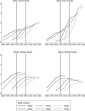
Figure 1 INTER- AND INTRA-REGIONAL MIGRATION OF SOUTHERN-BORN MEN, BY RACE AND BIRTH COHORT, 1880 TO 1960
In 1910, prior to the onset of the Great Migration, only 11 percent of black and white southern-born males in their 30s (the 1870s birth cohort) resided outside the South. For whites, this is approximately the same level of cumulative inter-regional migration as observed ten years earlier (in 1900) for men at a similar point in the lifecycle (the 1860s birth cohort). Later cohorts of whites undertook substantially more inter-regional migration: 15 percent of the 1890s birth cohort had left the South by 1930, and closer to 20 percent had left among those exposed to the WWII boom (observed in 1950). For blacks, the 1870s birth cohort had a slightly higher rate of cumulative inter-regional migration by 1910 than the 1860s cohort observed in 1900 (11 compared to 9 percent). That difference is dwarfed by subsequent changes in black inter-regional migration rates, with nearly one-quarter of the 1890s birth cohort leaving the South by 1930 and even higher rates for cohorts exposed to WWII (e.g., 36 percent of the 1910s birth cohort observed in 1950).
The comparatively low rate of inter-regional migration before 1910 does not imply that the southern labor force was stationary, as there is considerable evidence of mobility within the South (Wright Reference Wright1986). The lower panels of Figure 1 indicate that 15 percent of blacks and nearly 20 percent of whites in the 1870s birth cohort had moved away from their birth state by 1910 but stayed within the South. In this sense, intra-regional mobility was more common than inter-regional mobility prior to 1910. In particular, there were sizable flows of southern-born whites into Texas and Oklahoma and sizable flows of southern-born blacks into Florida, Arkansas, and Mississippi.
After 1910, flows within the South continued, especially to Texas, Oklahoma, and Florida, but destinations like California, Ohio, Illinois, Pennsylvania, and New York became much more prominent than previously. Between 1910 and 1930, Figure 1 shows slight declines in within-South migration but significant increases in inter-regional migration, reflecting a shift in the relative attraction of non-southern residence for both blacks and whites.
Scholars have suggested several reasons for the relatively low rates of African American migration from the South prior to WWI: low levels of human and financial capital, which have been found to impede long-distance migration in this and other settings (Logan Reference Logan2009; Hatton and Williamson Reference Hatton and Williamson2002); discrimination by northern employers who readily hired immigrant laborers from Europe (Myrdal Reference Myrdal1944; Collins Reference Collins1997); and weak integration of northern and southern labor markets compared to the strong ties between northern and European labor markets, a legacy of mass migration from Europe that began in the 1840s (Thomas Reference Thomas1954; Wright Reference Wright1986; Hatton and Williamson Reference Hatton and Williamson1998; Rosenbloom Reference Rosenbloom2002). Impediments to the mobility of southern agricultural workers also may have been significant (Ransom and Sutch Reference Ransom and Sutch1977; Grossman Reference Grossman1989; Naidu Reference Naidu2010).
Despite sizable inter-state flows of southern whites, the history of their internal migration has been far less explored than that of African Americans (Akers Reference Akers1936; Killian Reference Killian1953; Berry Reference Berry2000; Gregory Reference Gregory2005). Of course, some of the same factors that inhibited blacks' movement prior to WWI also may have affected southern whites. But it seems clear that the black and white stories differ in important ways. Most obviously, whites were not recently removed from slavery, were less concentrated than blacks in the Cotton Belt, were more likely than blacks to have acquired some wealth and literacy, and likely faced less discrimination in distant labor markets. For perspective, in 1870 nearly 40 percent of white southern men, age 20 to 60, owned some amount of real property, compared to less than 5 percent of blacks. Approximately 74 percent of southern whites (over age 9) could read and write, compared to 15 percent of blacks (Ruggles et al. Reference Ruggles, Alexander and Genadek2010). However, while southern whites might have found it easier to afford long-distance moves than blacks (on average), they also might have found it less attractive. For instance, opportunities to advance in southern labor markets, whether by ascending the agricultural ladder or moving into skilled non-agricultural work, may have seemed more plentiful to whites than to blacks. It is also possible that lingering hostility from the Civil War influenced white southerners' perceptions of the North.
If ignorance and poverty inhibited long-distance migration by black and white southerners, this constraint may have receded with each generation's educational and economic advances in the late nineteenth and early twentieth centuries (Higgs 1982; Margo Reference Margo1984, Reference Margo1990; Collins and Margo Reference Collins, Margo, Hanushek and Welch2006). In addition, improving transportation and communication networks in the South may have facilitated migration by lowering the associated costs and uncertainties. Surfaced roads more than doubled between 1904 and 1914 in the South (U.S. Department of Agriculture 1917). Nearly all southerners lived in counties with railroad access by 1911 (Atack Reference Atack2013 and personal communication). The circulation of northern newspapers, such as the Chicago Defender, increased in the South during the 1910s (Grossman Reference Grossman1989). Environmental shocks also may have driven some migration (Higgs Reference Higgs1976; Lange, Olmstead, and Rhode Reference Lange, Olmstead and Rhode2009; Boustan, Kahn, and Rhode Reference Boustan, Kahn and Rhode2012; Hornbeck and Naidu Reference Hornbeck and Naidu2014). Most prominently, the boll weevil spread from Texas, where it gained a foothold in the 1890s, to Mississippi by 1907 and North Carolina by 1919. The boll weevil disrupted cotton production and imparted a long-lasting negative productivity shock, perhaps making southern agriculture a less attractive option than before, at least within the Cotton Belt (Higgs Reference Higgs1976; Lange, Olmstead, and Rhode Reference Lange, Olmstead and Rhode2009; Baker Reference Baker2015). Finally, specifically for African Americans, political disenfranchisement, mob violence, de jure segregation, and, in general, the ascendance of the Jim Crow regime may have provided a strong incentive to leave the region (Myrdal Reference Myrdal1944; Woodward Reference Woodward1955; Kousser Reference Kousser1974; Tolnay and Beck Reference Tolnay1990; Margo Reference Margo1990). Taken together, these trends may have yielded a southern labor force circa 1910 that was more able and more inclined to migrate long distances than ever before.
Against this backdrop, the exogenous shock of WWI created both a major labor demand boom in industrial centers, predominantly located in the North, and a temporary halt to European immigration, which was later reinforced by immigration restrictions. Many industrial employers recruited southern migrants for the first time, gained experience in hiring, training, and evaluating them, and established networks to draw on the southern labor supply (Whatley Reference Whatley1990; Berry Reference Berry2000; Foote, Whatley, and Wright Reference Foote, Whatley and Wright2003). As is commonly found in studies of migration, networks of previous migrants helped perpetuate migration patterns in and from the South (Carrington, Detragiache, and Vishwanath Reference Hatton and Williamson1996; Hatton and Williamson Reference Hatton and Williamson1998; McKenzie and Rapoport Reference McKenzie and Rapoport2007). Consequently, high rates of migration continued long after the impetus of WWI, with major repercussions for American economic and social history.
Within this historical setting, our thinking about migration and location choice is guided by theoretical and empirical work by Larry A. Sjaastad (Reference Sjaastad1962), Jennifer Roback (Reference Roback1982), George J. Borjas, Stephen G. Bronars, and Stephen J. Trejo (Reference Borjas, Bronars and Trejo1992), Jeffrey Grogger and Gordon H. Hanson (Reference Borjas, Bronars and Trejo2011), and Enrico Moretti (Reference Moretti, Ashenfelter and Card2011). We suppose that an individual's location decision depends on expected income, amenities, and relocation costs (broadly defined), while recognizing that these expectations may vary across types of workers, by race, skill, or other initial conditions. These differences across workers may give rise to interesting patterns of selection into inter-state migration and of sorting across potential destinations, which we explore later. For both selection and sorting, the dataset of linked census records provides new opportunities for analysis.
NEW DATA: LINKING CENSUS RECORDS, 1910–1930
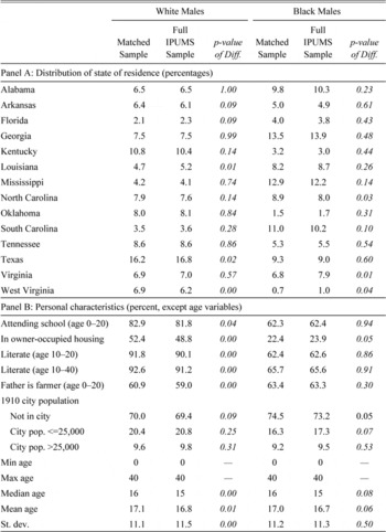
To construct the linked dataset, we began with the IPUMS sample of manuscript data from the 1910 Census of Population and selected all southern-resident males between the ages of 0 and 40 (Ruggles et al. Reference Ruggles, Alexander and Genadek2010). We then attempted to link these men “forward” by locating them in the handwritten manuscripts of the 1930 Census of Population. We used each individual's name, place of birth, and age from the 1910 records as search criteria for location in the 1930 records.Footnote 2 From an initial sample of 111,524 individuals, the linking process successfully located 26,829 individuals, a 24 percent match rate.Footnote 3 The final sample is 20 percent black. Additional details on the linking process and the variables available in each census year are provided in the Appendix.
As mentioned above, the linked data offer several advantages relative to the state-level aggregates or micro-level cross-sections that have typically supported quantitative studies of the Great Migration. The key distinction is that we observe the same person both before and after the onset of the Great Migration's first big wave. In 1910, we see the younger men in our sample when they still resided with their family. Therefore, we observe many characteristics about the household in which they grew up—what their parents did for a living, where they were located, whether they attended school, their literacy (if older than 9), whether they lived on a farm, and so on. The older men in our sample (18 and older) in 1910 are observed after they have left their parents, but also after they have entered the southern labor force. Therefore, we know what kind of job they held in 1910 in addition to whether they were literate, where they lived, whether they owned a home, and so on. In 1930, we see whether the men have moved since 1910 and, if so, to where. Given the 1910 county and state identifiers, it is straightforward to merge the linked dataset with 1910 county and state-level information from Michael Haines (Reference Haines2010), which helps characterize each individual's local economic and social environment.
A major concern for any such dataset is that the linked sample might exhibit selection bias that interferes with subsequent analyses and interpretations. Fortunately, the men in the linked sample are similar to those in the randomly selected base sample from 1910. Table 1 separately reports the summary statistics for the linked and base samples of blacks and whites. Although there are some small differences, their statistical and economic significance is limited. Similar conclusions follow when we estimate the probability of being in the linked sample as a function of observable characteristics, conditional on being in the base IPUMS sample. From that exercise (details of which are discussed in the Appendix), we conclude that literacy, farming occupations, and West Virginia residence are statistically significant predictors of being found in the 1930 census manuscripts, but the practical significance of these increased probabilities is small, generally less than a 3 percent increase.Footnote 4
Table 1 COMPARISON OF LINKED AND BASE SAMPLE CHARACTERISTICS, SOUTHERN MALES 1910
Notes:
A variance-ratio test is used to compare sample standard deviations and a Wilcoxon matched-pairs signed-rank test is used to compare sample medians. All others comparison of means are done with standard t-tests. The matched samples contain 21,367 white men and 5,462 black men.
Source:
The linked sample is created by taking the 1910 IPUMS sample of white and black males, age 0–40, who reside in the South and searching for these men in the 1930 census manuscripts. The text and Appendix describe sample construction in detail. The IPUMS data are from Ruggles et al. (Reference Ruggles, Alexander and Genadek2010).
A separate check with the 1930 IPUMS cross-sectional sample of southern-born black men, age 20 to 60 (to correspond to those 0 to 40 in 1910), reveals that 22 percent resided outside the South at the time of the 1930 census. This is close to the 20 percent of our matched sample who resided in the South in 1910 but not in 1930. We do not expect these numbers to be exactly the same because of interregional migration of men prior to 1910 in the IPUMS cross-section (where migrants are defined using place of birth information) and sampling variation. The corresponding numbers for southern-born whites observed outside the South in 1930 are 15 percent and 17 percent. Across all states, the distribution of inter-state migrants in the linked sample is highly correlated with inter-state migrants in the 1930 IPUMS sample (0.96 for both the white and black samples), and rarely deviates by more than 1 percentage point. The correlation is especially high for non-southern destinations, where pre-1910 migration is less likely to confound the comparisons (Appendix Table 3). Overall, the results do not suggest that the linked sample is biased in a way that will confound our analyses, and we take the linked sample to be fairly representative.
MIGRANT SELECTION
Patterns of migrant selection are important for both sending regions (e.g., whether the region tends to lose highly skilled workers) and receiving regions (e.g., whether migrants are likely to assimilate quickly and whether they are substitutes or complements for the area's native workers). The linked dataset is especially well suited to characterize selection into migration because it has such detailed background information on the men in 1910. These characterizations, in turn, provide a better basis than previously available for understanding the origins and consequences of the Great Migration, even though assessing the full range of possible implications from selection, such as the wage impact on sending and receiving areas (Boustan Reference Boustan2009), is beyond this article's scope.
In this section, we focus on characterizing who migrated and whether there are clear differences between migrants and non-migrants in terms of their background characteristics. We start by classifying all men in the linked sample into three mutually exclusive categories: “non-migrants” (who resided in the same state in 1910 and 1930), “within-South migrants” (who changed state of residence within the region), and “inter-regional migrants.” Between 1910 and 1930, a large fraction of the men in the linked sample (35 percent of whites and 39 percent of blacks) had left their 1910 state of residence, with roughly even splits between “within-South” and “inter-regional” migration.
Table 2, column 1 reports the white men's average characteristics in 1910, before the start of the Great Migration, including their literacy rates, school attendance, occupational income and education scores, farm status and homeownership rates. The figures are tabulated separately by 1930 migration category. The second column reports differences in characteristics between the migrant categories and the non-migrant category, and the third column reports the differences that remain after controlling for age and county-of-origin fixed effects.Footnote 5 In practice, the county-level fixed effects in column 3 absorb local push factors, such as boll weevil destruction, and control for selection that derives from differences in place-of-origin characteristics (which is included in the simple comparison in column 2).Footnote 6 The next three columns repeat the tabulations for the sample of black men. Although this is very basic information about the migrants and non-migrants, none of it can be inferred from census cross-sections, and in this respect the linked manuscript data are crucial.
Table 2 SELECTION INTO 1910–1930 MIGRATION ON BASIS OF 1910 CHARACTERISTICS

* = Significant at the 90 percent level.
** = Significant at the 95 percent level.
*** = Significant at the 99 percent level.
Notes:
“Adjusted differences” are regression coefficients that measure differences in 1910 characteristics among inter-regional, intra-region, and non-migrant categories (where non-migrants are the base category), controlling for age and county-of-origin fixed effects. Non-migrants are defined as residing in the same state in 1910 and 1930; within-South migrants left their state-of-origin but remained in the South. Literacy is recorded for those who are age 10 and over; school attendance is examined for 6 to 15 year olds. Occupational income and education scores are conditional on labor force participation in 1910. The standard deviation for occupation income score (occupation education score) is 12.0 (1.75) for whites and 7.3 (0.93) for blacks. Standard errors, clustered by county of origin, are in parentheses.
Source:
Data are from the sample of linked census records, as described in the text and Appendix.
If ability or productivity were positively correlated with migration, then we would expect migrants to have better outcomes than non-migrants in terms of human capital, occupational status, or family background before leaving the South. While discrimination in the South slowed black men's economic and educational progress, there was considerable variation in literacy, education, occupation, property ownership, and other measures in 1910. For whites and blacks, there is some evidence of positive selection into inter-regional migration on the basis of 1910 literacy (panel A), but the differences are quantitatively small at 1 to 4 percentage points. They are statistically insignificant after controlling for age and place of origin. This contrasts with some of the previous literature's suggestion of strongly positive migrant selection in the early twentieth century based on census cross-sections that observe migrants ex post (e.g., Tolnay Reference Tolnay1998). The discrepancy suggests that migrants might have improved their literacy after leaving the South, or that census enumeration of literacy might have been regionally biased. More generally, this raises concern regarding the practice of using ex post migrant characteristics from cross-sections to make inferences about selection into migration. As linked historical datasets become more common, scholars may be able to avoid this measurement problem.
For an alternative view of educational background, we examined school attendance in 1910 and found small differences in attendance rates between the migrant categories (panel B), with or without controls. From this perspective, migrant selection on the basis of formal education seems rather weak in the early decades of the Great Migration. We note, however, that in comparison to studies of migration in more recent decades (Borjas, Bronars, and Trejo Reference Borjas, Bronars and Trejo1992; Vigdor Reference Vigdor2002; Grogger and Hanson Reference Grogger and Hanson2011), which are often motivated by the Roy model (Reference Roy1951), our metric for educational attainment is fairly crude. We cannot follow such studies without better data for quality-adjusted educational attainment and variation in returns to education (by race) across locations in the early twentieth century, which to our knowledge does not exist.
Among those old enough to report occupations in 1910 (panels C and D), there is somewhat stronger evidence of positive selection on the basis of pre-Great Migration labor market outcomes. To the extent that better skills, ability, or motivation translated into better occupational standing before WWI, the occupational data provide a more sensitive indicator of selection than literacy alone. Individual income was not reported in the 1910 census, and so we first examine a modified version of the “occupational income score” (panel C).Footnote 7 This is a commonly used IPUMS variable that assigns an income to each detailed occupation category based on the median income observed in that occupation in the 1950 census (Ruggles et al. Reference Ruggles, Alexander and Genadek2010). Pre-war occupational scores for “within-South” and “inter-regional” white migrants are 5 to 10 percent higher than for non-migrants. For blacks, most group differences are slightly smaller in magnitude than for whites, but the point estimates are consistent with positive selection.Footnote 8
In panel D, we assign a race-specific “education score” to each detailed occupation in 1910 based on the average educational attainment of southern workers in the corresponding occupation categories in the 1940 census (Ruggles et al. Reference Ruggles, Alexander and Genadek2010), which was the first census to inquire about educational attainment. The goal is simply to provide an alternative characterization of occupational status that is connected to formal educational attainment rather than income. Again, there is some evidence of positive selection into migration, approximately one-tenth of a grade, but the differences are small and statistically insignificant after controlling for age and initial location.
In summary, our measures of skill—whether based on occupational or educational information—are generally consistent with a limited degree of positive selection for both whites and blacks in the early decades of the Great Migration. The differences across migrant groups are quantitatively small, however, and thus the degree of migrant selection from this perspective seems rather weak.
Table 2, panel E examines selection on the basis of farm status in 1910. From this perspective, there are notable differences. For both whites and blacks, those who lived on farms in 1910 were less likely to migrate out of the state than others. In the “unadjusted” columns, the farm-status difference between the migrant groups and the non-migrant group is between 7 and 11 percentage points (whites and blacks). The addition of age and county-of-origin controls reduces the gap relative to non-migrants for white inter-regional migrants and for both categories of African Americans migrants, but non-trivial differences remain, especially for whites. Thus, it appears that an agricultural background tended to hinder long-distance migration, even when comparisons are based on within-county variation.
Owner-occupied housing status, which is examined in Table 2's last panel, is of particular interest because it is the only census variable in 1910 that reflects household assets (ownership of real property). In general, household wealth may facilitate long-distance migration, but in this historical context homeownership may also indicate a prior decision to settle down in a particular area or, for young men in our sample (residing with their parents in owner-occupied housing), it may reflect an expectation to inherit or receive a parental gift of local property (Abramitzky, Boustan, and Eriksson Reference Abramitzky, Boustan and Eriksson2013). Among whites, residing in owner-occupied housing in 1910 is associated with substantially less long-distance migration (between 3 and 7 percentage points), even after adjustments for age and county of residence. African Americans were far less likely than whites to own their homes, and the pattern with respect to migration is different. Inter-regional black migrants were somewhat more likely to reside in owner-occupied housing in 1910. If the negative coefficients for whites are interpreted as indicators of relatively strong local attachments among property owners and their children, then it would appear that black property owners and their children did not share such strong attachments.
Overall, migration in the linked dataset does not conform to a simple characterization in terms of negative or positive selection. Migrants held jobs in 1910 with higher occupation scores than non-migrants on average, which is consistent with positive selection. But these differences were not large. Moreover, differences across migrant groups in terms of literacy, school attendance, or occupational-education scores were small or non-existent. Farm residence was the most robust (negative) predictor of subsequent migration for whites and blacks, a finding that is consistent with our expectations but novel in the sense that, to our knowledge, no previously constructed dataset could observe the pre-migration farm status of individual men in this period. We interpret the overall results as a reflection of remarkably broad participation in internal migration. The differences between migrants and non-migrants in the early decades of the Great Migration appear less salient than the increased volume and new directions of migration. This leads us to investigate further where the migrants moved and why they decided to move there.
OVERVIEW OF MIGRATION PATTERNS AND SORTING
The linked dataset provides new opportunities for studying and comparing migrant sorting patterns, both as a function of individual and place-of-origin characteristics and as a function of labor market conditions and migration costs across space. In addition, the linked data allow us to be more specific about when people moved (between 1910 and 1930) than is possible with census cross-sections, where prior location is known only at the time of birth and migration could have occurred at any time afterwards.
Table 3 provides summary statistics of the migration patterns in the linked dataset, including the propensity to migrate (panel A) and distance and direction of migration (panel B). The table's third column reports simple black-white differences. The fourth column reports coefficients on a black indicator variable from regressions that control for state-of-origin fixed effects. As mentioned above, between 1910 and 1930, a large fraction of the men in the linked sample left their 1910 state of residence, with approximately an even split of migrants between “within-South” and “outside South” destinations. Among those who left the South, the Midwest was the most common destination for both whites and blacks, but black inter-regional migrants moved relatively strongly into the Northeast (compared to whites), whereas whites moved relatively strongly into the West.Footnote 9 Detailed state-to-state migration patterns are reported in the Online Appendix.
Table 3 MIGRATION PATTERN SUMMARY STATISTICS, BY RACE: 1910–1930

Notes:
The last column reports regressions coefficients that compare black and white migration patterns controlling for state-of-origin fixed effects. The “full sample” includes non-migrants (defined as those who do not leave the state-of-origin). South-to-Northeast includes 1930 residents of the Northeast census regions and also Delaware, Maryland, and Washington, DC. Latitude differences are positive for south-to-north migration. Longitude differences are positive for west-to-east migration. Standard errors, clustered by county of origin, are in parentheses.
Sources:
Data are from the linked sample of census records, as described in the text and Appendix.
Panel B of Table 3 reports measures of distance travelled based on the latitude and longitude of the center of each individual's 1910 and 1930 county of residence. In the full sample, average migration distances, including zeros for those who did not change counties, are similar across the black and white samples, with or without controls for state-of-origin. It is clear, however, that conditional on migrating, whites moved farther than blacks on average, both within the South (322 versus 266 miles) and when leaving the South (696 versus 577 miles) (also see Tolnay et al. Reference Tolnay, White and Crowder2005). Controlling for state-of-origin amplifies the large difference in distance travelled by inter-regional migrants (column 4). The average black male moved northward and eastward (positive changes in latitude and longitude), whereas the average white male moved northward and westward, though not as far north as blacks. Among white inter-regional movers, the migrants to the West strongly influence the average change of longitude, and black-white differences in east-west mobility patterns are striking, even when controlling for state of origin.Footnote 10
For the sake of concise description and to facilitate discrete-choice modeling, we focus on the migrants' choice of state. In our sample 51 percent of inter-state migrants chose non-urban locations, and therefore focusing solely on migrants to cities would omit a large share of the sample, distort the ex ante set of destination choices, and generally mischaracterize the period's internal migration patterns. Moreover, because the multinomial logit model, described below, estimates a large number of coefficients for each potential destination, working at the county- or city-level would be computationally prohibitive.
Figure 2 maps the distribution of inter-state southern migrants across destinations between 1910 and 1930. Continuing pre-1910 migration trends, migrants within the South tended to favor Texas, Oklahoma, and Florida, with Texas and Oklahoma being particularly important destinations for whites. In addition, and breaking with pre-1910 patterns, black migrants frequently chose locations in the industrial North; Pennsylvania, Illinois, Ohio, and New York all received more southern black migrants after 1910 than did any southern state. Pennsylvania was the most common destination for blacks, and it drew heavily from Virginia, Georgia, and South Carolina. Southern white migrants were also drawn strongly to Ohio and, to a lesser extent, Illinois. But California also emerged as a major destination for whites, drawing heavily from the 1910 residents of Texas, Oklahoma, Arkansas, and Kentucky.

Figure 2 DISTRIBUTION OF INTER-STATE MIGRANTS IN LINKED SAMPLE, 1910–1930
Although there was a substantial degree of overlap in black and white migration flows, there were also notable differences among the most frequently chosen locales. Only Ohio and Illinois rank among the top five destination states for both groups, and in some cases the black-white differences are quite large (e.g., California and Pennsylvania). A dissimilarity index provides a simple way to summarize the magnitude of black-white differences in the migrants' location choices. It indicates the share of migrants that would have to choose a different location for the distribution of choices to be the same across race categories. The index is calculated as 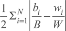 where i denotes a state, b
i
(w
i
) is the number of black (white) men moving to state i and B (W) is the total number of black (white) migrants in the sample. From this perspective, approximately 28 percent (index value of 0.28) of black or white inter-state migrants would have to choose a different destination for the black and white post-migration distributions to be equivalent.
where i denotes a state, b
i
(w
i
) is the number of black (white) men moving to state i and B (W) is the total number of black (white) migrants in the sample. From this perspective, approximately 28 percent (index value of 0.28) of black or white inter-state migrants would have to choose a different destination for the black and white post-migration distributions to be equivalent.
BACKGROUND CHARACTERISTICS AND DIFFERENCES IN BLACK AND WHITE MIGRATION PATTERNS
Because black and white men differed in their observable characteristics and starting locations circa 1910, it is natural to ask whether such differences can account for black-white differences in migration patterns. We take two different approaches to this question. First, looking deeper into the summary statistics reported in Table 3, we estimate a series of ordinary least squares (OLS) regressions that include a race indicator variable and a rich set of background variables, such as age, literacy, industry of employment (or father's industry of employment), place of origin, and so on. Comparing “unadjusted” black-white migration differences to those “adjusted” for background characteristics, we find that the background characteristics generally cannot account for the differences in migration outcomes. In fact, adding control variables tends to widen, not narrow, some black-white differences in migration choices. For the sake of brevity, these results and additional details are provided in the Online Appendix.
Second, similar in spirit to the above but with a sharper focus on the actual choice of destination, we estimate multinomial logit models to characterize the location choices of inter-state migrants as a function of race and background characteristics. The multinomial framework treats each state as a potential destination, with the caveat that we combined some less populous states to facilitate estimation. For the subsample of individuals age 17 and under in 1910, the model includes indicator variables for race, father's literacy and industry of employment, own school attendance, place in the family's birth order, owner-occupied housing status, state of origin, and city size. For those 18 and older in 1910, the list of independent variables is similar, but includes own literacy and industry of employment (rather than father's) and marital status, but omits school attendance and birth order. The Online Appendix provides more details.
Using the model's parameter estimates, the importance of black-white disparities in observable characteristics is revealed by comparing two counterfactual migration distributions in which men have the same characteristics except for race. Specifically, we take the full sample of white and black men and predict destination choices when all are assigned “black” status and then again when all are assigned “white” status, such that the differences across the two sets of predictions are attributable only to differences in race as all other personal attributes are equivalent across counterfactuals (StataCorp 2009). For each man, this procedure estimates probabilities of choosing each state under white and black model parameters; the probabilities are averaged to get the predicted “all white” or “all black” counterfactual distributions of migrants across states. If differences in background characteristics largely explained black-white differences in destination choice, then the value of the dissimilarity index between the all black and all white counterfactual distributions would be substantially less than the index value based on the actual distributions. In practice, however, recalculating the dissimilarity index between the “all black” and “all white” counterfactual distributions yields an index value of 0.27. From this perspective, only a small portion of black-white differences in destination choice, on net, can be accounted for by the background characteristics available in the census. Underlying the dissimilarity index results, we see that background characteristics are helpful in narrowing the black-white difference in migration to some states (most notably California), but they widen the black-white difference in other states (such as Illinois and Missouri), such that the overall dissimilarity index changes little.Footnote 11
In sum, we find that there was substantial overlap in black and white migration patterns, but black-white differences in migration patterns were economically significant and generally were not a reflection of the migrants' background characteristics. Observationally similar southern men circa 1910 tended to make different migration decisions depending on their race. This finding leads us to focus on how strongly (and how differently) white and black migrants responded to variation in the costs and benefits of relocating to each potential destination. Conditional logit models are particularly useful for studying such issues.
CONDITIONAL LOGIT MODEL OF DESTINATION CHOICE
Suppose that individual i chooses to migrate to state j if
where U(˙) represents utility over a vector X ik , which contains variables that reflect the expected income, amenities, and migration costs for individual i in potential destination k. If the utility over each state choice includes a random component with an Extreme Value Type I distribution, the probability of choosing any particular state is represented by:
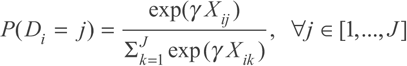
where D i is the location choice of individual i. This is the familiar conditional logit framework for discrete choice described in Daniel McFadden (Reference McFadden and Zarembka1974), applied to a setting in which migrants choose destinations (Davies, Greenwood, and Li Reference Davies and Greenwood2001; Vigdor Reference Vigdor2002; Wozniak Reference Wozniak2010). As cited earlier in the article, our interpretation of the model in this setting is strongly influenced by previous research on the economics of migration and location choice (Sjaastad Reference Sjaastad1962; Roback Reference Roback1982; Borjas, Bronars, and Trejo Reference Borjas, Bronars and Trejo1992; Grogger and Hanson Reference Grogger and Hanson2011; Moretti Reference Moretti, Ashenfelter and Card2011).
Maximum-likelihood estimates of γ describe how differences in economic characteristics across potential destination states are correlated with the choices of inter-state migrants. Note that in conditional logit models, any variable that does not vary across potential destinations for individual i, such as an individual-specific variable or place-of-origin-specific variable, falls out of the estimating equation and is not identified. Coefficients on destination-specific characteristics and on interactions between destination characteristics and individual-specific attributes can be identified (e.g., interactions of labor demand and race).
We estimate the conditional logit model with the sample of inter-state migrants. We do not include non-migrants in the analysis because doing so poses conceptual problems with key variables such as “distance” and “migrant stock” and with the treatment of “home” as a potential destination choice. Since this section of the article is primarily concerned with describing the migrants' choices of destinations rather than their selection into migration, we believe that concentrating on the migrants simplifies the analysis and the interpretation of variables in a way that is helpful.Footnote 12
Several variables comprise X ij , starting with those that may have influenced expected employment opportunities and earnings. We construct a measure of post-1910 labor demand growth (B j ), following Timothy Bartik (Reference Bartik1991). In Bartik's specification, employment growth in each state is predicted by multiplying the size of the 1910 labor force in each industry in each state (e jl ) by a 1910–1930 nationwide employment growth rate in that industry (g l ), and then summing across industries within states.
The Bartik-style measure gauges total employment growth in each state without utilizing ex post state-specific labor force growth rates, which are endogenous to migration. We also estimate specifications that include the percentages of the 1910 labor force employed in agriculture and manufacturing separately rather than the Bartik measure, which combines information over all industries. In the specifications with agriculture and manufacturing employment variables, we also include a control variable for state population size because larger states are likely to attract more migrants all else equal.
The vector X ij also includes race-specific income estimates for each state circa 1910. These measures combine state-level estimates of real income per worker from Kris James Mitchener and Ian W. McLean (Reference Mitchener and McLean1999) with race-specific adjustment factors for each state that are calculated from the 1940 census microdata (the first census year with wage data).Footnote 13 In essence, the output-per-worker benchmark in each state circa 1910 is scaled up or down depending on the ratio of black or white men's wages to all wages in that state in the 1940 census. The Online Appendix provides more detail.
Variables related to the cost of migration are also in X ij . We calculate the log distance from each individual's county of residence in 1910 to each potential destination state to capture relocation costs that are proportional to (log) distance. In addition, we calculate the share of all people born in person i's home state who resided in state j in 1910, separately by race, using the 1910 IPUMS (Ruggles et al. Reference Ruggles, Alexander and Genadek2010). These pre-1910 migration rates help account for the influence of pre-existing and race-specific relationships between states including, but not limited to, networks that facilitate migration by providing a cultural home and assistance with finding employment and housing.
A regional dummy variable for “Non-South” captures the influence of region-specific amenities, some of which may have differentially influenced decisions of black and white migrants, such as more secure civil rights or less rigid social segregation. The coefficient reflects migration above or below what would be expected on the basis of the economic variables included in X ij . This is a simple way to test whether areas outside the South were especially attractive to southern migrants, conditional on other X variables. Of course, identifying this border effect relies upon the sample's inclusion of both intra-regional and inter-regional migrants, and identifying a race-specific border effect relies upon having both white and black migrants. The theme of escaping the South is prominent in many narrative descriptions of African Americans' motives for inter-regional migration (e.g., Wilkerson Reference Wilkerson2010), but others have noted that racial oppression long preceded the onset of the Great Migration (Higgs Reference Higgs1976; Vickery Reference Vickery1977). Whether areas outside the South were especially attractive to black migrants and whether that influence can be detected after controlling for economic conditions are open empirical questions. In subsequent analysis, we estimate separate coefficients for the Northeast, Midwest, and West (rather than treating the Non-South as a single region) or with a full set of destination fixed effects.
The baseline analysis also includes a variable for each state's level of urbanization to see whether migrants were drawn to highly urbanized states for reasons that are not captured by other independent variables. Robustness checks with different specifications and functional form assumptions are discussed later and in further detail in the Online Appendix.
CONDITIONAL LOGIT RESULTS
The baseline results are presented in Table 4. Columns 1 to 3 pertain to the sample of white men, columns 4 to 6 pertain to black men, and columns 7 to 9 pool the samples and report coefficients on X variables interacted with a race dummy variable (black=1) to highlight differences. Models in columns 3, 6, and 9 include destination-state fixed effects. The presence of state fixed effects limits the set of coefficients we can identify to those that vary across individuals within potential destinations, which means we cannot identify most of the X variables' coefficients in this specification. Nonetheless, because distance and migrant-stock variables do vary within destination categories across individuals, their coefficients are identified, and the specification provides a useful robustness check.
Table 4 MIGRANT SORTING, CONDITIONAL LOGIT COEFFICIENTS

* = Significant at the 90 percent level.
** = Significant at the 95 percent level.
*** = Significant at the 99 percent level.
Notes:
The sample includes inter-state migrants from the linked dataset of census records. Columns 1–3 include white men. Columns 4–6 include black men. Columns 7–9 report interaction terms from a pooled regression with each regressor interacted with a race dummy (1=black). Specifications A and B differ in the inclusion/exclusion of labor demand, log population, percent manufacturing and percent agriculture variables only. Specification C includes potential destination state fixed effects. Distance refers to county of resident in 1910 to population-weighted center of each potential destination state. Migrant stock refers to the share of persons born in state i who are residing in state j in 1910 (calculated with IPUMS, Ruggles et al. Reference Ruggles, Alexander and Genadek2010). The labor demand variable follows Bartik (Reference Bartik1991) and uses 1910 industry composition at the state level to form a weighted average of national-level industry-specific growth rates. Log average income combines information from Mitchener and McLean (Reference Mitchener and McLean1999) and the 1940 census microdata (Ruggles et al. Reference Ruggles, Alexander and Genadek2010), as described in the text and Appendix. Non-South equals one for destination states outside the South, including Maryland, Delaware, and Washington, DC. Percent of labor force in manufacturing and agriculture, percent urban, and total population in 1910 are from Haines (Reference Haines2010). Standard errors, clustered at the county of origin, are in parentheses.
Sources:
Data are from the linked sample of census records, as described in the text and Appendix.
A positive logit coefficient indicates that an increase in that variable for a particular state is associated with an increase the probability of migration to that state. Interpreting the magnitude of logit coefficients is not straightforward, and therefore we present some counterfactuals to illustrate the results. For reference, marginal effects for each variable for each destination state and race are reported in the Online Appendix.
Across all specifications and both races, migrants responded negatively to distance and positively to pre-existing stocks of migrants from the same state. Black migrants appear to have been more strongly deterred by distance than whites, and this difference is statistically significant even when controlling for pre-existing migrant stocks and destination fixed effects. The relatively strong response to distance may reflect southern blacks' lower average levels of wealth and educational attainment, which could affect their access to information about distant opportunities and their ability to finance long-distance travel. It is noteworthy, however, that splitting the black sample into literate and illiterate men (in 1910) does not reveal a statistically significant difference in their migration behavior with respect to distance (Online Appendix Table 8), nor does splitting the sample by 1910 homeownership status. For perspective on the magnitude of the distance coefficients in columns 1 and 4 of Table 4, the results suggest that if southern migrants had been located one standard deviation farther away from Ohio (all else held constant), then the share of migrants going to Ohio would have declined by 3 percentage points for whites and 4 percentage points for blacks, relative to a base of 8 and 7 percentage points respectively.Footnote 14 The average “marginal effect” over all destination states (equally weighted) is –1.15 percentage points for whites and –1.43 points for blacks for a one-standard deviation change in log distance. The empirical importance of distance suggests that improvements in transportation and information networks played an important role in facilitating internal migration and integrating U.S. labor markets.
The black and white coefficients on the pre-existing migrant stock variable are positive, similar across specifications, and not statistically different from one another in columns 7 to 9. Thus, responsiveness to migrant networks measured in this manner did not distinguish blacks' migration behavior from that of whites. However, blacks and whites' pre-existing migrant stocks were distributed differently. Therefore, networks might still have been an important determinant of differences in flows.Footnote 15 The results are fairly similar in specifications with destination fixed effects (columns 3 and 6), suggesting that the migrant stock coefficients in other specifications are not simply picking up destination-specific unobservables that had drawn previous migrants. For some states, especially those that had relatively small stocks of previous southern migrants, plausibly sized changes in the migrant-stock variable do not imply large changes in the predicted flow of migrants between 1910 and 1930. In California, for example, increasing the black migrant-stock variable's value to equal that of whites (within each state of origin) would raise California's share of black migrants from 1.8 to 1.9 percent. This accounts for little of the sizable racial difference in migration to California (5 percentage points). However, in some other states, the implications of scaling up the stock of previous migrants are larger. Increasing the black variable's value to equal that of whites for Texas would raise Texas's share of black migrants from 3.8 to 7.8 percent (compared to a share of 10.3 percent for whites). The average marginal effect of a one standard-deviation change in pre-existing migrant stock over all states is 0.45 percentage points for whites and 0.33 points for blacks.
The results in columns 1 and 4 of Table 4 indicate that white and black migration was strongly correlated with exogenous variation in aggregate labor demand growth. The positive response to this variable is no great surprise because booming labor markets are commonly cited as motivation for long-distance migration and, in general, large states tend to have large changes in employment and, therefore, attract large shares of migrants. It is interesting that black men appear to have been highly responsive to this signal relative to white men (column 7), perhaps reflecting the relative importance of finding employment quickly upon arrival or extra weight given to this signal as a correlate of changing employment opportunities for blacks specifically (i.e., relative to previous discriminatory practices in northern and western labor markets). For perspective on the coefficient, if Tennessee's labor demand had grown one standard deviation faster, the estimates suggest that its share of black migrants would have increased by 5 percentage points relative to a base of 5 percent; for whites, the predicted increase is 2 percentage points relative to a base of 4 percent. Given a one-standard-deviation change in labor demand, the average marginal effect over all potential destination states is 1.10 percentage points for whites and 2.27 points for blacks.
In columns 2, 5, and 8, we enter separate variables for manufacturing and agricultural employment shares in 1910, rather than aggregate employment growth, to provide a different perspective on the economic characteristics of states that may have influenced migration patterns. Black men were inclined to select states with high levels of manufacturing employment, but disinclined to select agricultural states, all else the same. It is notable that the coefficient on manufacturing is positive even when a “Non-South” dummy variable, urban share, and average income are included as independent variables in the specification. In other words, the positive manufacturing coefficient for blacks suggests that the sector itself was an important determinant of black migration patterns. For white men, both the manufacturing and agricultural coefficients are negative in column 2, suggesting that they tended to seek residence in states with higher levels of employment in “other” industries, such as construction, mining, trade, transportation, and services.
We also estimate models that distinguish among parts of the South that were differentially affected by the spread of the boll weevil. We defined three groups of states depending on their cotton intensity and the boll weevil's time of arrival. We considered states “cotton intensive” if at least 20 percent of total crop value came from cotton production in 1910 (Haines Reference Haines2010). Based on the map from Walter Hunter and B.R. Coad (Reference Hunter and Coad1923), we coded Texas, Arkansas, Louisiana, and Mississippi as “early boll weevil” states. They were cotton intensive and received the boll weevil prior to our window of observation (before 1910). We coded Alabama, Georgia, South Carolina, North Carolina, and Oklahoma as “late boll weevil” states. They were cotton intensive and received the boll weevil after 1910, within our window of observation. The third group is comprised of Tennessee, Kentucky, Virginia, West Virginia, and Florida, which were not cotton intensive.Footnote 16
If the boll weevil imparted a long-lasting negative productivity shock that is not captured by control variables and was not neutralized by cotton price changes or the redistribution of economic activity to other crops or sectors, then we would expect to see less migration to cotton-intensive places in our sample, ceteris paribus. We find that relative to states where cotton was less important (the omitted category), blacks and whites were both less likely to move to cotton-intensive states (with the exception of blacks in specification B), consistent with a negative and persistent productivity shock across cotton-producing regions.Footnote 17 Coefficients are more negative for the “late” boll weevil states than for the “early” boll weevil states, but the differences between “late” and “early” state groups are not statistically significant.
In Table 4, the coefficients on the average income variable, which varies by destination state and race, are positive but somewhat weaker in specifications that include controls for industrial composition. The coefficients in columns 1 and 4 imply that a one-standard-deviation increase in income in Pennsylvania would have raised its share of white migrants by about 2.6 percentage points and its share of black migrants by about 1.7 percentage points, relative to base shares of 3 and 8 percent, respectively. Columns 7 and 8 suggest that white migrants were more responsive than blacks to variation in pre-war income. It is possible that whites, perhaps because they had higher levels of education or access to more information, were better informed than blacks about wages in distant states and, therefore, more responsive to the existing variation. But again, there is no evidence that literate blacks were more responsive than illiterate blacks to variation in average income (Online Appendix Table 8). Another possibility is that the estimates of race-specific income circa 1910 are a better proxy for whites' expected earnings opportunities after 1910 than for blacks.
For both white and black men in columns 1, 2, 4, and 5 of Table 4, the coefficient on the Non-South variable is negative. Taken at face value, neither white nor black southern migrants were especially attracted to the Non-South, conditional on other X variables.Footnote 18 There is some concern that controlling for pre-existing migrant stocks may absorb some of the attraction of regional amenities to the extent that previous migrants responded to those same amenities. However, omitting the migrant-stock variable from the specifications in columns 4 and 5 has little effect on the Non-South coefficient for black migrants (not shown). In columns 7 and 8, the coefficients on Non-South interacted with race (black=1) are not statistically significant, which again runs counter to some of the literature's emphasis on the idea that black migrants were especially motivated to escape the South (beyond that which is embedded in the other X variables).Footnote 19
A more nuanced picture emerges by separately estimating coefficients for Northeast, Midwest, and West (expressed relative to South), instead of just “Non-South.” Estimates of these coefficients are located in Table 5. Black migrants were significantly more attracted to the Northeast and Midwest than whites conditional on the other X variables, but they were significantly less likely to move to the West. Thus, the “Non-South” variable in Table 4 tends to mask substantial unexplained differences in blacks' and whites' choices of sub-region outside the South. These residual differences in migration might reflect differences in labor market discrimination, civil liberties, or social norms across northern and western locations after 1910, a hypothesis that merits further research. In this interpretation, white migrants serve as a control group to capture the influence of unobserved, race-neutral subregional characteristics, so that black-white differences might then be interpreted as evidence of race-specific factors that vary over subregions. Note that for blacks (columns 3 and 4) the coefficients for Midwest and Northeast are still negative (expressed relative to the South), but they are smaller in magnitude than the negative coefficients for whites.
Table 5 MIGRANT SORTING, CONDITIONAL LOGIT COEFFICIENTS ON REGIONAL INDICATORS

Notes:
All regressions also include corresponding covariates reported in Table 4, with the exception of the “Non-South” indicator. Regional definitions follow standard census regions with the exception of Delaware, Maryland, and Washington DC, which we classify as “Northeast” rather than “South.” See notes to Table 4 for more details.
Sources:
Data are from the linked sample of census records, as described in the text and Appendix.
Returning to Table 4's results, in columns 1 and 4, the coefficient on “urban” is negative for white men but positive for black men. The coefficients suggest small effects on migration patterns. Raising Mississippi's urban share by one standard deviation (22 percentage points) would raise its share of black migrants by only 0.5 percentage points, relative to a base of 3.5 percent. Because urbanization is highly correlated with manufacturing and agricultural employment, we do not emphasize the coefficient on urban in columns 2 and 5.
In sum, the article's earlier analysis found that it was not possible to account for differences in white and black migration patterns with the individuals' background characteristics. Instead, the different patterns must have resulted from differences in perceived opportunities and migration costs across space (X) and differences in how men responded to those opportunities and costs (γ). To gauge how much of the black-white differences in destination choice can be accounted for by distance and migrant stock variables, we apply the parameters of the black conditional logit model with destination fixed effects to all men in the sample (black and white), and then apply the parameters of the white model to all men.Footnote 20 This yields two counterfactual distributions of migrants with the same underlying X values. The dissimilarity index of the two counterfactual distributions is approximately 0.20, substantially less than the unadjusted index value of 0.28. From this perspective, equalizing the migrant-stock and distance variables across black and white migrants reduces the dissimilarity index by about one-fourth. The remaining differences in migration patterns reflect differences in race-specific wages across states (absorbed by race-specific destination fixed effects) and model coefficients (the γ's), which are difficult to interpret definitively. Nonetheless, we believe that additional research could isolate and test specific hypotheses and interpretations (e.g., whether the pattern of black-white differences in destination fixed effects correlates with a measure of local labor market discrimination, perhaps following Sundstrom Reference Sundstrom2007).
CONCLUSION
To study migration patterns during the first decades of the Great Migration, we built a new dataset of more than 26,000 southern men that we linked from the 1910 to the 1930 census. The dataset is novel in that it observes the same men before and after the start of the Great Migration. The scope of analysis is novel in that it includes both white and black southerners and it incorporates information about those who moved within the South as well as those who left the region.
First, we study selection into inter-state and inter-regional migration. There is some evidence of positive selection into migration among both whites and blacks in terms of occupational status, and it is clear that non-farm residents (in 1910) were more likely to move across state and regional lines than farm residents. Overall, however, the differences between migrants and non-migrants were small within race categories, even for those moving inter-regionally. In this sense, participation in internal migration by southern men was remarkably widespread after 1910.
Second, we examine migration patterns between origins and destinations and ask whether individual and local background characteristics account for differences in black and white migration choices. Although there was substantial overlap in black and white migrants' choices of destinations, there were also notable differences. In OLS and multinomial logit frameworks, we find that on net a surprisingly small amount of the black-white differences in migration patterns can be accounted for by differences in background characteristics. In other words, to the extent that black and white migration patterns differed, those differences were not, in general, a simple reflection of where the men started geographically or their personal circumstances circa 1910. Rather, observationally similar men made different location choices depending on their race.
Third, given the findings above, we measure black and white migrants' responsiveness to variation in the characteristics of potential destinations. Black and white men were similarly responsive to pre-existing migrant stocks, but black men were more deterred by distance than whites, more attracted to manufacturing centers, and more responsive to variation in labor demand growth. Conditional on the potential destination states' characteristics, we find only mixed evidence that black migrants were more likely than whites to leave the South. There is, however, interesting variation across areas outside the South, with blacks sorting more strongly than whites into the Midwest and Northeast and whites sorting more strongly into the West, conditional on state characteristics. Variation in the characteristics of potential destinations, such as distance and pre-existing migrant stocks, can account for a non-trivial portion of the black-white dissimilarity index in destinations, but a larger portion is associated with racial differences in responsiveness to the destinations' characteristics and in destination fixed effects. These differences invite further research.
The article's findings rely heavily on the linked dataset of census records for southern males from 1910 to 1930, and it is our hope that other scholars will find this dataset to be useful. We have endeavored to keep the analyses focused on a set of fundamental questions about the nature of internal migration in this period, but it is not difficult to imagine extensions that look at finer levels of geographic detail, exploit more information on the migrants' outcomes, or link to other historical or administrative datasets. More generally, it is clear that this kind of dataset holds great promise for historical research on migration (e.g., Ferrie Reference Ferrie2005; Abramitzky, Boustan, and Eriksson Reference Abramitzky, Boustan and Eriksson2012), and new technologies and initiatives are likely to make them far more common and accessible in the future. Lying just beyond the scope of this article, there is much that remains to be learned about migration during the Great Depression, the growth of black ghettos and suburbanization of whites, the interaction of migration and intergenerational mobility, and much more. All these topics are ripe for reassessment as new datasets that follow individuals over time are brought to light.
Appendix
For each male, age 0 to 40, in the 1910 IPUMS sample (Ruggles et al. Reference Ruggles, Alexander and Genadek2010), we ran two searches in the 1930 census manuscripts: one with exact last name and one with a SOUNDEX version of the last name. In both cases, we conditioned on the first three letters of the first name (or less, if shorter than three letters in length), exact state of birth, age within two years, race, and gender. We counted any individual with a unique match in the exact last name or SOUNDEX search as a successful match. We then eliminated all duplicate matches (i.e., two different individuals in 1910 linked to the same individual in the 1930 census).
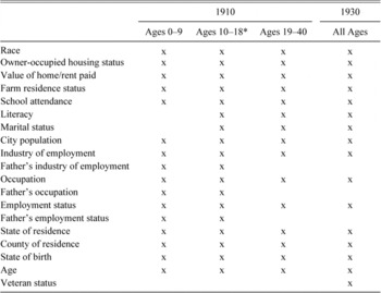
From the 1930 census, we extracted detailed location of residence as well as information on literacy, employment, occupation, industry, and veteran status. Individual and household-level variables available in the linked sample are detailed in Appendix Table 1. The availability of some variables depends on an individual's age at the time of enumeration. And although some variables are technically “available” for all age groups, they are practically missing (e.g., occupation for 0–9 year olds).
Appendix Table 1 VARIABLE AVAILABILITY, 1910–1930 LINKED SAMPLE OF CENSUS RECORDS
The characteristics of males in the matched sample are compared to those of the entire 1910 IPUMS sample in Table 1 of the main text. There, we concluded that the differences are not economically significant and are unlikely to bias the study of migration patterns. Here, we also provide estimates of a linear probability model of being found in 1930 (out of those in the original IPUMS sample), conditional on observable 1910 characteristics. The results are located in Appendix Table 2 and largely echo the conclusions from Table 1 in the main text. Specifically, we estimate the probability of being located in the 1930 manuscripts separately by race and three age categories: 0–9, 10–18, and 19–40. The age groupings correspond to the availability of school attendance, literacy, and farming occupation information in the 1910 data. We observe a slightly increased probability of being found for literate individuals, farmers, and residents of West Virginia, conclusions highlighted in discussion of Table 1, as well. On the other hand, homeownership is a statistically insignificant predictor of sample inclusion conditional on other factors observable in 1910. In each case, the enhanced probability of being located in the 1930 manuscripts is small: 0.78–2.4 percentage points in the case of literacy and 2.0–2.9 percentage points for farming occupations. Residence in West Virginia in 1910 raises the probability of being located in 1930 by as much as 5.5 percentage points, but for a relatively small number of men (6.2 percent of white males in the sample lived in West Virginia in 1910).
Appendix Table 2 ESTIMATED PROBABILITY OF INCLUSION IN MATCHED SAMPLE, BY AGE GROUP AND RACE

In Appendix Table 3, we compare the 1930 characteristics of inter-regional migrants in the linked sample to those in the 1930 IPUMS sample. The matched sample's inter-regional migrants are individuals with a southern state of residence in 1910 and a non-southern residence in 1930. IPUMS migrants, on the other hand, are individuals with a southern place of birth and a non-southern residence in 1930. Thus, individuals who migrated out of the South prior to 1910 will not be included in our sample but will be included in the IPUMS sample. We cannot correct for these fundamental sample differences.Footnote 21 Nonetheless, the differences across samples are small even when they are statistically significant. The most notable exception is the share of white migrants in owner-occupied housing in the linked sample (38 percent) relative to the 1930 cross-sectional sample (33 percent). As mentioned in the main text, when comparing destination shares in the linked and cross-sectional datasets (separately for black and white inter-state migrants), the correlation in migration patterns is high. With inter-regional destination states grouped as in Appendix Table 1, the correlation is more than 0.98 for both whites and blacks.
Appendix Table 3 COMPARISON OF LINKED AND FULL SAMPLES, SOUTHERN MIGRANTS TO THE NON-SOUTH, 1930


