


Introduction
High-resolution, in situ techniques for determination of mineralogy and elemental composition are highly desirable on upcoming space missions. Difficulties regarding mineral determination in situ are mainly related to the strong heterogeneous character of natural rock samples, making direct interpretations complex. Presently, many chemical and mineralogical determinations of rocks are done from bulk material of ground-up samples. This is not only time and energy consuming but also destructive. The need for high-resolution, high-precision techniques is therefore compelling. In this study, a miniaturized laser ablation mass spectrometer (LMS), designed for in situ space research (Rohner et al. Reference Rohner, Whitby and Wurz2003; Riedo et al. Reference Riedo2013b; Tulej et al. Reference Tulej, Iakovleva, Leya and Wurz2010, Reference Tulej, Riedo, Iakovleva and Wurz2012, Reference Tulej2014) is shown to be useful for the measurement of elemental composition and its spatial variations, both laterally and with depth, in a strongly heterogeneous rock sample. Because of the LMS' high dynamic range, small crater sizes and simultaneous measurement of all elements (Riedo et al. Reference Riedo, Bieler, Neuland and Tulej2013a, Reference Riedob), we can show the spatial compositional variation of individual grains and minerals. In this way, it is possible to determine not only the mineralogy of a sample on very small spatial scales but also the degree of weathering and alteration. Using such a minute amount of sample the technique is practically non-destructive and has the potential to be very useful when analysing natural, highly heterogeneous rock samples in situ on rocky extraterrestrial planetary bodies.
Material and methods
The sample used for this study is amygdaloidal pillow basalt from Kinghorn, Fife, Scotland with an approximate age of 360–320 Ma (McMahon et al. Reference McMahon, Parnell and Blamey2012). The basaltic lavas from the Fife area consist of highly weathered basalts with olivine, pyroxene (augite) phenocrysts. The olivine phenocrysts are mostly pseudomorphed to calcite and quartz (Rex & Scott Reference Rex and Scott1987). The sometimes glassy groundmass consists of calcic plagioclase and anhedral titano-magnetite. Amygdales in basaltic lavas are usually formed through gas bubble release when the lava is cooling and the pressure is released upon eruption. After the cooling of the lava, hydrothermal fluids pass through the cavities (vesicles) and precipitate secondary minerals (usually calcite, zeolites and/or quartz), which then become the amygdales.
Polished thin sections (thickness of approx. 30 µm) were prepared from the samples. The sample was chosen to be as representative for extraterrestrial conditions as possible. Mafic rocks are the predominant rock type on terrestrial-like planets such as Mars. Veins and voids in basalts have also been recognized as habitats for endolithic microorganisms, whose remains usually are found in secondary in-filling mineralizations such as carbonates (Ivarsson et al. Reference Ivarsson, Bengtson, Belivanova, Stampanoni, Marone and Tehler2012). The current sample contains filamentous micro-structures similar in size and occurrence to microbial filaments. Despite not being remains of microorganisms their occurrence in secondary carbonates and their morphologies make them excellent specimens to test the instrument for future studies of true microfossils. Mineralogy and microstructures were localized and analysed using optical microscopy, environmental scanning electron microscopy (ESEM) coupled with an energy dispersive spectrometer (EDS) on an FEI QUANTA FEG 650 (Oxford Instruments, UK). For the analysis by EDS, an Oxford T-Max 80 detector was used. No coatings of the samples were used during ESEM/EDS analyses. To minimize surface charging effects, the sample was kept at low vacuum conditions and the acceleration voltage was kept at 20 or 15 kV depending on the nature of the sample. The instrument was calibrated using a cobalt standard. Peak and element analyses were done using INCA Suite 4.11 software. A fragment of the thin section (approximately 2 × 3 mm2) was mounted onto a stainless-steel sample holder with copper tape for chemical analyses using a LMS. The LMS combines a laser ablation/ionization ion source with a reflectron-time-of-flight mass analyser (Rohner et al. Reference Rohner, Whitby and Wurz2003). The full technical details of the instrument are described in previous publications (Riedo et al. Reference Riedo, Bieler, Neuland and Tulej2013a, Reference Riedob, Reference Riedo, Neuland, Meyer, Tulej and Wurzc; Neuland et al. Reference Neuland, Riedo, Meyer, Mezger, Tulej and Wurz2013, Reference Neuland, Meyer, Mezger, Riedo, Tulej and Wurz2014). Here we used a focused femtosecond (fs) laser (τ ~ 190 fs, λ = 775 nm, laser pulse repetition rate ≤1 kHz) for ablation and ionization of the sample (Grimaudo et al. Reference Grimaudo, Moreno-García, Riedo, Neuland, Tulej, Broekmann and Wurz2015). Typical sample consumption is below picograms. The software used for operating the LMS system controls the laser pulse energy, laser pulse repetition rate and number of laser pulses, and is described in an earlier publication (Riedo et al. Reference Riedo, Bieler, Neuland and Tulej2013a). An x-y-z micro-translation stage was used for positioning the sample under the laser ablation location with a positioning accuracy of about ±20 µm. The spot diameter was about 15 µm and the applied energy per pulse was 6 µJ, which resulted in a laser irradiance of 42 TW cm−2. Quantitative elemental composition and derivation of the mineralogy of the sample with lateral and vertical resolution were made investigating a sequence of ten points on the sample separated by 20 µm from each other (see Fig. 1). The size of investigated area is defined by the laser spot diameter. The ablation studies were performed by applying 40 000 laser shots at each location. A total of 200 mass spectra were collected, each being the sum of 200 single-shot spectra. Hence, an individual depth layer is defined as a depth range ablated by 200 consecutive laser shots. The thickness of a depth layer depends strongly on the ablation rate, i.e on the laser fluence and its absorption by the sample. For the investigated sample the ablation rate is observed to increase steadily from location 1 (carbonate host) to location 2 (amygdale inclusion). Based on the results from our recent studies the ablation rate for carbonate material is expected to be in the range 0.01–0.1 nm per laser shot whereas for locations on the darker surface the ablation rate is 1–5 nm per laser shot (Grimaudo et al. Reference Grimaudo, Moreno-García, Riedo, Neuland, Tulej, Broekmann and Wurz2015). For the purpose of the current analysis these estimates should be sufficiently accurate and a more accurate determination of the ablation layer thickness was not attempted. The elemental composition of an individual ablation layer or the average over all the measured layers was determined from the mass spectra using the procedure described in another publication (Riedo et al. Reference Riedo, Bieler, Neuland and Tulej2013a).

Fig. 1. Optical images showing the (a) entire sample including the host basalt (BAS), the amygdale (AM) and the TFS and (b) placement and numbering of the points investigated by LMS in the dark inclusion resembling a tangle of filamentous structures (TFS).
Mineralogical analyses were made using a Horiba instrument LabRAM HR 800 laser Raman confocal spectrometer equipped with a multichannel air-cooled charge-coupled device (CCD) detector. An Ar–ion laser (λ = 514 nm) was used as the excitation source. The instrument was integrated with an Olympus microscope and the laser beam was focused to a spot of 1 µm with a 100x objective and with a spectral resolution of about 0.3 cm–1. The instrument was calibrated using a neon lamp and the Raman line (520.7 cm–1) of a silicon wafer. Instrument control and data acquisition was made with the LabSpec 5 software.
Synchrotron radiation X-ray tomographic microscopy (SRXTM) was performed at the tomographic microscopy and coherent radiology experiments (TOMCAT) beamline of the Swiss Light Source at the Paul Scherrer Institute, Villigen, Switzerland. The X-ray energy was 20 keV, and 1501 projections were obtained over 180°. An LSO : Tb 5.9 µm scintillator and a 40× lens were used, resulting in a voxel size of 0.1625 µm. Reconstruction was based on the Fourier Transform method (Marone & Stampanoni Reference Marone and Stampanoni2012). Slice data were analysed and rendered using Avizo™ software.
Results and discussion
Optical microscopy and X-ray Tomography
A colourless mineral (amygdale, AM) with a dark inclusion resembling a tangle of filamentous structures (TFS) was observed using an optical microscope (Fig. 1(b)). The filaments propagate outward in all directions from a central point. They have a diameter of 0.2–3 µm and vary in length from a few micrometres to up to 150 µm. Tomographic reconstructions of the TFS clearly showed a characteristic millerite (a NiS mineral with a profound acicular habit, commonly associated with serpentine rocks) structure (Fig. 2(a)–(c)) and that there is an overgrowth of brush-like structures covering the millerite structure, especially close to the middle of the TFS. Small denser grains can also be seen both within the TFS and in the surrounding calcite. The SRXTM revealed that the apparent filamentous structure of the TFS seen under optical microscopy (Fig. 2(a) and (b)) in fact consists of pin-straight, even crystals and are thus not organically formed filaments as implied from optical microscopy. Branching was seen using SRXTM (see red arrows in Fig. 2(c)). The entire TFS inclusion is about 200–300 µm in size.

Fig. 2. SRXTM volume renderings showing the morphology, branching and size distribution of the crystals that constitute the TFS and, where (a) shows the entire TFS and arrows pointing on the ‘brush-like’ structures, (b) shows a zoomed-in region where the straight crystal shapes are clearly visible and (c) shows the branching of some crystals (white arrows).
ESEM/EDS
ESEM/EDS elemental mapping revealed elemental concentration differences between the TFS and the surrounding amygdale host rock, Fig. 3. At least three different phases were observed in the TFS; (1) long, needle-shaped structures consisting of Ni-Co-Fe-S (NS), 2) Structureless parts consisting of only Si and O and (SiO), and 3) Phases containing Al-Mg-O-Fe that surround the needle-shaped crystals (ALP).

Fig. 3. ESEM mapping of the TFS, showing the distribution of key elements in the sample. The upper picture is a compilation of the maps of S, Si, Fe, O and Ca.
Raman
The Raman analyses identify the host basaltic rock as composed of clinochlore ((Mg5Al)(AlSi3)O10(OH)8), plagioclase (NaAlSi3O8–CaAl2Si2O8), clinochlore-transformed augite ((Ca,Na)(Mg,Fe,Al,Ti)(Si,Al)2O6), anatase (TiO2) and calcite (CaCO3). This is in agreement with the published data (Geikie & Peach Reference Geikie and Peach1900; Rex & Scott Reference Rex and Scott1987). The amygdale mineral is a calcite, which is also reported in the literature (Geikie & Peach Reference Geikie and Peach1900). The ESEM measurements suggest that Mn is a consistent but minor part of the calcite (Fig. 3), but no Raman spectrum can confirm a Mn-bearing calcite, or a Mn-carbonate.
The long, needle-shaped structures are identified as millerite, a nickel-sulfide mineral (NiS), by Raman spectroscopy (Fig. 4), and SIO is identified as poorly crystalline quartz. Highly weathered amygdaloidal, basaltic samples are consistent with the presence of millerite, which is a low-temperature calcite- and serpentine-associated mineral (Moody Reference Moody1976; Anthony Reference Anthony, Bideaux, Bladh and Nichols1990; Schwarzenbach & Früh-Green Reference Schwarzenbach, Früh-Green and Bernasconi2009), and quartz is a documented pseudomorph of the olivine phenocrysts (Rex & Scott Reference Rex and Scott1987). The ALP phase was identified to represent the mineralogy of the basaltic host rock to a large extent but in general, chlorite was surrounding the millerite crystals.

Fig. 4. Raman spectrum showing the spectrum from the TFS (a mixture of millerite and calcite) in black, the reference spectrum for millerite in red and reference spectrum for calcite in light blue.
LMS
Mass spectra were collected in the low-gain (LG) and high-gain (HG) channel (see Riedo et al. Reference Riedo, Bieler, Neuland and Tulej2013a, Reference Riedob, Reference Riedo, Neuland, Meyer, Tulej and Wurzc) from all ten locations on the sample. As an example the mass spectrum from spot number 6 is shown in Fig. 5. The LG channel records the major elements, which in this case are H, C, O, Na, Mg, Al, Si, S, K, Ca, Fe, Co and Cu. These mass spectra can be interpreted as CaCO3 with additions of quartz, clinochlore and other minor minerals. Mn was associated with CaCO3 and is identified in the LMS data where it is present already in the LG channel and much better seen in the HG channel (Fig. 5), which confirms that Mn is not a major, but a minor, species in the CaCO3 mineral. The HG channel shows the ratio D/H2 and the minor elements Li, B, C, O, Na, Mg, S, Mn, Fe, Ni and carbon clusters, which are all identified in Fig. 5.

Fig. 5. Mass spectrum of the LG and HG channels showing major and minor elements present in the sample in spot number 6. With observed dynamic range close to 106 the detection of elements with the concentrations down to ppm level are expected.
In the following, we discuss the variation of elemental abundances within the investigated depth layers and locations with relevance to mineralogy. Figures 6–10 summarize the results of the measurements performed at each location, 0–9, and the variation of the mass peak intensities of several elements are plotted between the location numbers. The mass spectra provide information on chemical composition change from one to the other location and also compositional changes with the depth. The apparent differences in mass peak intensities between ablation points 0–4 and 5–9 are due to the different ablation rates at these locations, which affected the measurement sensitivity. An increase of laser irradiance would be necessary to increase the ablation rate at the calcite site, but this would result in a decrease in spectral quality on millerite surfaces. The composition of the surrounding host material in the amygdale was known and a decision was made to optimize the laser fluence to the TFS area instead.

Fig. 6. Relative variation of oxygen with depth and proximity to the centre of TFS showing ablation points 0–4 in (a) and ablation points 5–9 in (b).

Fig. 7. Relative variation of (a) sulphur and (b) iron with depth and proximity to the centre of TFS.

Fig. 8. Relative element composition from LMS mass spectra for all ablation points showed in Fig. 5b represented both laterally by the integers at the x-axis giving the ablation point, and with depth (data between the integers with lowest number representing the surface). (a) Shows the relative abundances of Si, S and Fe, (b) O, Al, Ca and (c) Mg, Ni and Co.

Fig. 9. Relative element composition from LMS mass spectra for all ablation points showing the correlation of elements making up specific minerals identified in the sample using Raman spectroscopy. The format is the same as in Fig. 7. (a) shows arrows pointing on locations with overlaps of Co, Ni and S indicative of millerite, (b) shows arrows pointing on locations with overlaps of Ca, C and O indicative of calcite, and (c) shows arrows pointing on locations with overlaps of O and Si indicative of quartz.

Fig. 10. Relative elemental composition from LMS mass spectra for all ablation points showing the correlation of elements in minerals identified by Raman spectroscopy. The format is the same as in Fig. 7. (a) arrows pointing on locations with overlaps of Fe and O indicative of iron oxide, (b) shows data for Ti and O and the locations where the O/Ti ratio = 2 indicative for anastase, and (c) shows the data for Fe, Mg and Al.
The measurements at the first four locations were performed in the pure amygdale calcite, where the mass peaks of the elements C, Ca and O were observed to be the most intense in the mass spectrum and other elements are present in the mass spectra at a minor level. Calcium and O are present and coincide also throughout the entire ablation profile with several other elements. Their abundance ratios are consistent with the composition of calcite.
The oxidizing conditions increase linearly with the proximity to the TFS centre (Fig. 6), which is consistent also with the formation processes associated with the amygdaloidal pillow basalts. The negative correlation between S and Fe in contrast to the ESEM analysis indicates that there are no pyrite in the sample, which is confirmed by the Raman spectra where no pyrite could be observed (Fig. 7(a) and (b)). ESEM analyses are semi-quantitative and has a broad beam spot that may include elements to the spectra outside the target area, which is why Fe and S seems to appear together in the ESEM mapping figure (Fig. 3).
The amount of S increases linearly with the proximity to the TFS centre, Fig. 7(a), but the spatial variation for S and Fe does not show the same pattern. Instead, Fe and O coincide perfectly, which is consistent with the presence of iron oxides (Fig. 7(b)). The major elements appearing in the ESEM maps are S, Si, Fe, O, Ca, Al, Ni, Co and Mg are also present in mass spectra of all ablation points. Fig. 8 shows the analysis of all mass spectra for these elements in three panels for the locations given in Fig. 1(b).
Figure 8(c), shows that Ni and Co are strongly correlated throughout the entire data set, confirming the Raman observations of millerite (Fig. 4). Cobalt is closely correlated to Ni in the entire profile, but since no Co-bearing mineral phase was found with Raman spectroscopy this is likely a substitution of Ni for Co, which is a common feature in millerite (Ineson Reference Ineson2014). This means that both Ni and Co will be present and positively correlated with S because of their mutual association in the mineral.
To confirm the presence of the minerals derived from the Raman analyses, element correlation analyses are presented assuming that characteristic elements of these minerals can be identified in the LMS mass spectra, which are shown in Figs 9 and 10. In Fig. 9(a), the elements Ni, Co and S are positively correlated almost throughout the entire data set but it is most pronounced in the ablation points 2–6. Thereafter, there are some points in which the correlation is negative, where S is very high compared with Ni and Co. From these analyses of the mass spectra one can conclude that millerite is present at least on the edges of the TFS, but likely also inside the TFS. Calcite is mostly identified in the ablation points 0–5, as expected, since calcite is the dominating mineral there and the interferences of other elements are not so profound see Fig. 9(b). Quartz can possibly be observed as increased Si signals correlated with an increased O signal, see Fig. 9(c).
Figure 10(a)–(c), show the relative abundance of elements indicative of the location of iron oxides, anatase and chlorite minerals. The O abundance is loosely tracing the Fe abundance, especially at ablation points 7 and 8, suggesting that iron oxides are present in the sample, which is consistent with the literature from the area (Rex & Scott Reference Rex and Scott1987). However, the location of anatase and chlorite is not unambiguous as many elements show high abundance in the TFS. Our Raman spectrum showed the presence of both anatase and chlorite within the TFS and the elements appearing in those minerals correlate also in the LMS element data (Fig. 10(b) and (c)). In Fig. 10(b), markings have been added to show the positions where the O/Ti ratio is 2 (which represents the anatase O/Ti ratio). From those points, it can be seen that the O/Ti ratio is 2 mostly outside the TFS, indicating that the anatase is coupled to the calcite rather than to the TFS. This indicates that anatase is syngenetic with the calcite and that the TFS is a later alteration product. The increase of O in the TFS with increasing ablation numbers (Fig. 8(b) and Fig. 9(b) and (c)) shows that at least some parts of the TFS are oxidized, which is also confirmed by the presence of iron oxides and alteration products such as clinochlore.
A detailed depth profile analysis is presented for location 4 and 7 in Fig. 11. Typically, at one measurement location the measured mass peak intensities of the analysed elements are observed to decay smoothly with the ablation progress (ablation number layer) when homogenous material is investigated. In the current studies, the peak intensity envelope is generally more complex. The measurements yield relatively large peak intensity variations are indicating a deficit or increase of the concentration of particular elements for particular ablation layer. From the analysis of element correlation (element deficit, element concentration increase) one can get an insight into mineralogical composition of the investigated layer.
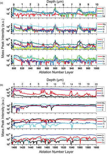
Fig. 11. Variation of mass peak intensities of various elements with ablation depth measured at location 4(a) and 7(b).
The chemical compositional analysis of the first uppermost surface layers measured at location 4 shows no significant relative variation of elemental peak intensities. All peak intensities decay with relatively similar rate, and only very small variations can be seen for these uppermost surface layers. However, at location 7, larger intensity variations are observed. The peak intensities of the elements B, C, O and S decrease steadily with the ablation progress while the mass peak intensities of the other elements are observed to increase; they reach their highest intensities after ablation of approximately 20 layers, thereafter the intensities decrease.
Occasionally, at some depths (at some ablation layers) the peak intensities of some of the elements were observed to increase and others to decrease. At location 4 an increase of peak intensities was observed in the ablation layer ranges 814–820, 830–846, 894–910 and 952–968, respectively. In the depth layer range 865–874, the sulphur intensity is readily decreasing while intensities of other element increase. Large peak intensity variations were observed at location 7 for several ablation layers including 1435–1445, 1465–1488, 1535–1540 and 1570–1590. For these depth layers, an increase in intensity of several elements (including B, C, O, Na, S and Ti) is accompanying a decrease in the peak intensities of other measured elements (Mg, Al. Si, K, Ca, Cr, Fe, Ni and Co). The correlation and anticorrelation indicate presence of chemically different layers or particles. While changes of the intensities of several elements at location 4 (left panel) are relatively well-correlated, at location 7 (right panel) for some of the elements the intensities are anticorrelated. The depth scale is roughly estimated for these locations and leads to the conclusion that the size of these layers/particles is in the range 1–3 µm. The correlation of elements in ablation point number 4 indicates a fast precipitation, in which the calcite was precipitating quickly together with all other elements and no other minerals had the time to form. At ablation point 7, several minerals are present, indicating enough time for minerals (in this case, mainly secondary) to form and precipitate. The elements Mg, Si, Al, V, Ca, K, Co, Cr and Ni are anticorrelating with C, B, O, Na, S and Ti, which suggests a secondary mineralogy forming anatase, sodium carbonates and sulphates, whereas the heavier metals remained within the carbonates during the alteration of the amygdales. This is contradictory to the interpretation of the O/Ti ratio, where anatase was suggested to be syngenetic with the calcite. The solubility of Na, Ti, S, B and C ions is higher than that of the other elements, and it is therefore more likely that anatase is syngenetic with the secondary mineral precipitation than with the calcite. The oxidation of the minerals at point 7 is much higher than at point 4, suggesting that the alteration of the amygdales is through oxidative fluids.
The relative abundances of elements measured at the location 3–7 are presented in Table 1 and displayed in Fig. 12. The elemental analysis at each location was computed from the mass spectrum obtained by summing up the spectra of individual ablation layers.

Fig. 12. Elemental abundance fractions at several locations for major (a), minor (b) and trace elements (c, d).
Table 1. Abundance of elements for locations 3–7 (see Fig. 12) determined from the mass spectrometric analysis. Elements with concentrations down to ppm level are measured (Ca, F and Cl)

In general, many elements are correlated at the same ablation points, and only large deviations may be considered as tenable mineral identification. The size of the ablation crater is likely playing a role in that the ablated materials are picking up signals not only from the structures but also to a large extent from the surrounding host minerals, since the ablation spot size is larger than the thickness of the filaments.
The analyses of depth profiles from each spot are shown between the integer ablation numbers on the x-axis in Figs 8–10. The oxidation of the surface is clearly visible as high O signals at the surface followed by a rapid decrease with depth, except from ablation points 7 and 8, where the O is high throughout the investigated depth layers, indicating the presence of oxidized minerals such as iron oxides. With the first layer discarded, there are still strong sulphur signals with depth, showing repeated occurrence of S-rich grains with minor additions of Ni and Co (Fig. 12).
Conclusions
In general, the LMS mass spectra, the Raman spectra and the ESEM data provide consistent information about the elemental and mineralogical composition of the sample as well as syngenicity and oxidation properties. This suggests that LMS is an instrument by which in situ analyses of mineralogical composition are highly conceivable. The data from the LMS also show that this is not purely a surface analysis technique, but LMS also provides detailed depth information making it a high-resolution, in situ, three-dimensional-analysis technique for elemental composition. This is of great importance for in situ analyses of heterogeneous material on rocky extraterrestrial bodies during future space missions. LMS delivers highly sensitive elemental analysis with high lateral and vertical resolution. This study demonstrates its capability to conduct depth profiling of geological samples with sub-micrometre resolution. These offer new perspectives for context analysis and the detection of micrometre-sized grains/layers, and open new possibilities for the investigation of grain elemental and mineralogical composition.
Acknowledgements
This work has been funded by Swedish National Space Board (Dnr 100/13) and the Swiss National Science Foundation. We would additionally thank Marianne Ahlbom for the help with ESEM analyses.


 Open access