2.1 Flagging and calibration

The MWA band is comprised of 3 072 10 kHz ‘fine’ channels, derived from 24 1.28 MHz ‘coarse’ channels. The eight edge fine channels of each coarse channel suffer aliasing and are flagged in every observation. The central fine channel of each coarse channel contains the (non-zero) DC component of the polyphase filterbank, so is also flagged. Known misbehaving antennas were flagged, and the Orbcomm transmission frequency range 136–138.5 MHz was completely excised. Radio-frequency interference was excised using aoflagger (Offringa, van de Gronde, & Roerdink Reference Offringa, van de Gronde and Roerdink2012); due to the radio-quiet nature of the observatory, less than 3% of the data were affected and removed, mostly at the 136–138 MHz range of the Orbcomm satellite downlink. From a native frequency resolution of 10 kHz, the data were averaged by a factor of four in frequency, appropriately downweighting any frequency bin containing a reduced number of fine channels. From the original time-sampling of 0.5 s, gamma data were averaged by a further factor of two in time, while beta data were time-averaged by a factor of eight, the difference arising from the larger number of long baselines in gamma.

A single calibration solution was determined for each frequency, for each night, based on the calibrator listed in Table 1.

2.2 Subtraction of bright sources in primary beam sidelobes

The first sidelobes of the MWA primary beam are estimated to have a response of approximately 3% of that of the main beam, and the second around 0.1% (see Section 3.5 for more details on the primary beam model). When an extremely bright source such as Cygnus A passes through such a sidelobe, it contributes signal to the visibilities. If not subtracted directly from the visibilities (‘peeled’) or deconvolved, this contribution is visible in the image as striping from the sidelobes of the synthesised beam at the position of the source. In the absence of computing constraints, one could attempt to image the entire sky, such that all sources are deconvolved. However, we found that bright sources sufficiently far (> 45°) from the phase centre were poorly deconvolved even in a snapshot image due to the array not being perfectly coplanar. At the time of analysis, techniques such as w-projection (Cornwell, Golap, & Bhatnagar Reference Cornwell, Golap and Bhatnagar2008) were too computationally expensive for the ~ 10 000 pixel-wide grid required to cover the sky. The sidelobes also introduce a large spectral variation to the image pixels, as they vary much more quickly with frequency than the main beam.

To reduce the effects of bright sources in the sidelobes of the primary beam, we phase-rotated the calibrated, concatenated snapshot datasets to the source positions and performed a shallow (threshold = 10 Jy) clean of a 1° × 1° around each source, with an additional Taylor term, allowing each pixel to have its own spectral index (Sault & Wieringa Reference Sault and Wieringa1994). The model pixels were then subtracted from the visibilities, which were then phase-rotated back to their original positions, ready for imaging. The sources removed in this way were Pictor A, the Crab Nebula, Hydra A, Cygnus A, PKS2153 − 69 and PKS2356 − 61. Only Pictor A was present in the primary beam main lobe, as well as the sidelobe, and we note that this strategy means we are then unable to recover its flux density in the final mosaic.

2.3 Imaging strategy

At 150 MHz, the full-width half maximum (FWHM) of the MWA primary beam at zenith is approximately 30°, corresponding to more than two hours of RA. Sources therefore appear in many of the two minute scans as the sky drifts through the beam. Within any two-minute scan (hereafter a ‘snapshot’), the hybrid beta/gamma array is sufficiently coplanar that snapshot images do not suffer from wide-field effects within the main primary beam lobe (< 15° from the phase centre) and the image coordinates can be described by a slant-orthographic (generalised SIN) projection (Perley Reference Perley, Taylor, Carilli and Perley1999; Calabretta & Greisen Reference Calabretta and Greisen2002). The data were thus divided into snapshots with the phase centre defined as the local sidereal time in the middle of the snapshot. The goal of data processing is to form an image of the entire RA range of the observation using all of the available data.

Given the drift scan observation strategy, standard synthesis imaging techniques are not suitable. In a drift scan, instead of pointing the beam at adjacent locations on the sky, the beam stays constant and the sky moves, relatively. The data are therefore best processed using a mosaicking methodology. Typically the goal of a mosaic observation is to image objects larger than the primary beam of the telescope (e.g. Holdaway Reference Holdaway, Taylor, Carilli and Perley1999). Much of the mosaicking literature and software is therefore focused on recovering the large-scale structure in a synthesis image using an interferometer with very short baselines. In the case of these data, the commissioning sub-array has only 12 baselines shorter than 20 m and thus sensitive to scales > 5°, unlike the full MWA which fully samples up to scales of 12° (at 180 MHz). As we are also observing a part of the sky mostly devoid of objects of large angular scale, our focus is on combining the data to maximise sensitivity to compact structures.

To form the mosaic images, we perform the following steps, for each frequency band, for each polarisation:

• • generate an output accumulation image for the data and primary beam in an equal area coordinate system with 0.5 arcmin pixel resolution and over a sufficient region of the sky for all data;

• • for each snapshot:

  • – invert using multi-frequency synthesis over a field-of-view of 40° × 40°, with a pixel resolution of 1 arcmin, weighting each u, v-cell equally (‘uniform weighting’);

  • – clean to a threshold of three times the typical snapshot root-mean-square (RMS), which itself is typically ≃ 240–80 mJy beam^{− 1} from 120–180 MHz; the synthesised beam sidelobes are only ≈ 10% of the peak response, and a gain factor of 0.1 is used, thus avoiding cleaning the noise, and clean bias;

  • – restore using an elliptical Gaussian approximation of the snapshot synthesised beam;

  • – regrid and add the deconvolved image multiplied by the appropriate primary beam model into the accumulation data image;

  • – likewise, regrid and add the square of the beam image into the accumulation beam image;

• • after all additions, divide the data image by the beam-squared image to form the final mosaic.

In essence, this follows Equation (1) from Sault, Staveley-Smith, & Brouw (Reference Sault, Staveley-Smith and Brouw1996) which maximises the signal-to-noise ratio (S/N) in the output mosaic given the changing S/N over the field in each snapshot due to the primary beam. We use the miriad for the imaging, deconvolution and image arithmetic, and use our own code to generate MWA primary beam models (see Section 3.5 for more details on the primary beam model). miriad’s understanding of advanced World Coordinate Systems (WCS) and ability to regrid between arbitrary coordinate frames is especially useful.

The process of adding snapshots improves the quality of the final image by reducing the thermal noise and improving the synthesised beam, revealing many fainter sources. These fainter sources have not been deconvolved in the snapshots, so their sidelobes remain in the mosaic with ~ 1 h of effective earth rotation synthesis (the time it takes for sources to move through the utilised area of the primary beam). We estimate the (5σ) classical confusion limit (Condon Reference Condon1974) to be approximately 5 mJy beam^{− 1} given our effective synthesised beam size; this is consistent with the confusion measurement by Bernardi et al. (Reference Bernardi2009, Reference Bernardi2010) at 150 MHz at a similar angular resolution and frequency. While we therefore begin to approach the classical confusion limit, the dominant components of noise in our mosaics are sidelobe confusion and calibration errors. A randomly-chosen section of the 180 MHz Dec − 47 mosaic is shown in Figure 3, showing the well-behaved point spread function (PSF) and averaging down of calibration errors that results from the mosaicking process.

Figure 3. A randomly-chosen section of the 180 MHz Dec − 47 pseudo-Stokes I mosaic, representing about 4% of the total MWACS survey area (in one of the three frequency bands). The greyscale is linear and runs from − 0.2 to + 0.8 Jy, and the estimated PSF at the centre of the image is shown as a boxed filled ellipse at the bottom-left of the image, of dimensions 4.31 arcmin × 2.94 arcmin, position angle − 50.°4. Some calibration errors are still in evidence, particularly around the bright source in the north–west. MWACS detections are shown as white ellipses of the same shapes as their fitted Gaussian parameters. The RMS of this image is 28 mJy.

The zenith-pointed MWA primary beam is virtually identical for the XX and YY polarisations. We therefore averaged the XX and YY Dec − 27 mosaics to form a (pseudo) Stokes I image. For the Dec − 47 mosaic, we found that the primary beam response of the XX and YY polarisations was sufficiently different that Dec-dependent corrections were required. Hence, the XX and YY mosaics for Dec − 47 were not combined at this stage. Details of this process and absolute calibration are discussed in Section 3.5.

3.1 Sensitivity

Maps of the RMS value of the 180 MHz mosaic pixels were generated using aegean (Hancock et al. Reference Hancock, Murphy, Gaensler, Hopkins and Curran2012) which calculates the RMS for blocks of pixels with dimensions of approximately 20 × 20 beamsFootnote ⁴ . These are reproduced for two representative mosaics in Figure 4 (see also Figure 16). Two effects can clearly be seen in these figures: an increase in RMS at the edges of the mosaics, and isolated patches of locally high RMS. The first is due to the effect of the primary beam and the second is due to the effect of sidelobe confusion and calibration errors around the brighter sources. The latter is particularly severe near extremely bright, resolved structures which can most easily be seen close to the Galactic plane (at the easternmost edge of the Dec − 47 scan). Fornax A produces more calibration-error noise in the Dec − 27 scan, and less in the better-calibrated Dec − 47 scan; deconvolution errors from poorly reconstructing the largest scales of its structure are present in both.

Figure 4. Log-scaled images of the RMS intensity measured across the mosaics for the highest-frequency Dec − 27 (top) and Dec − 47 (bottom) scan. The greyscale runs from 0.02 to 0.4 Jy beam^{− 1}. The north–south axis is Dec in decimal degrees, and the east–west axis is RA in hours.

3.2 Source identification

We wish to identify and characterise the morphology and flux density of all sources within the field which are bright enough to be discerned from the background noise. Having characterised the noise properties of the mosaics, we identify those pixels of the mosaics whose flux is greater than five times the local RMS, which itself is hereafter denoted σ. blobcat (Hales et al. Reference Hales, Murphy, Curran, Middelberg, Gaensler and Norris2012) was used to identify ‘blobs’: islands of pixels containing a 5σ peak, expanded to include all contiguous pixels brighter than 3.5σ, while accounting for various biases.

This was repeated for all three (Dec − 27, Dec − 47 XX and Dec − 47 YY) of the highest frequency (180 MHz) mosaics. These were used exclusively for source-finding since the highest resolution allowed the greatest separation of neighbouring sources into discrete blobs. The objects detected in the three maps were combined into a single list (i.e. from this point on no regard was taken as to which map the source was detected in).

3.3 Characterising the point spread function

For an interferometer coplanar to the plane perpendicular to the zenith, observing at zero hour angle, the synthesised beam becomes elongated N-S relative to the zenith, as csc ζ, where ζ is the zenith angle. Regridding from a slant orthographic projection to a zenithal equal area projection (using standard miriad WCS tools) conserves the synthesised beam volume, ignoring this effect, such that a correction factor of csc ζ must be applied to rescale the N-S extent of the synthesised beam. We apply this immediately, before making further measurements.

While the synthesised beam shape for an individual snapshot is known very accurately (short-timescale ionospheric effects aside), determination of the effective synthesised beam in the mosaics is a much more difficult problem. The mosaic contains approximately an hour (depending on frequency) of effective earth rotation synthesis which significantly circularises the PSF. However, refraction from the ionosphere acts differently in each snapshot and enlarges the PSF as snapshots are combined to form each mosaic.

To measure this effect, we fitted 2D Gaussians to all detected sources, and plotted the distribution of ellipse values against various parameters (such as RA, Dec) and checked for correlations: none were seen. Plotting against S/N, as in Figure 5, shows that the ellipse sizes of unresolved sources form a line, with the resolved sources having larger values. For each Gaussian parameter, a line was fitted to the unresolved sources, and compared with the predicted value in order to calculate the correction needed to increase the size of the PSF to match the data.

Figure 5. An example of the analysis used to find the correct PSF for the mosaicked images: in this case, we examine the major axis of sources detected in the zenith scan at 180 MHz. The black crosses show the measured major axis of each source against its S/N; the grey stars show the expected major axis if the zenith-angle-dependent projection effect were the only source of change in the synthesised beam; the light grey dashed line shows a S/N-weighted horizontal fit to the major axis measurements. The ratio of this fit to the predicted major axis gives the correction factor by which the major axis of the PSF must be increased to match the data: see Table 2 for a list of the corrected PSFs for each mosaic.

Table 2. Gaussian parameters for corrected PSFs for the mosaics, at their original phase centres. The Dec − 47 entries apply to both the XX and YY mosaics.

Henceforth, all source-finding uses the corrected PSFs, shown in Table 2. Note that the PSFs are identical for the XX and YY polarisation Dec − 47 mosaics, as all of these effects are polarisation independent. A further projection factor of csc ζ is applied when measuring sources in the mosaics. Figure 6 shows an exaggerated illustration of the effect of these changes. After these corrections, it is possible to recover the flux densities of extended sources, which would otherwise be over- or under-estimated depending on the difference between the local PSF and average PSFFootnote ⁵ .

Figure 6. An exaggerated example of the corrections made to the PSF: the solid black ellipse shows a 150 MHz synthesised beam at the zenith; the dashed line shows the synthesised beam for a pointing due south, at a zenith angle of 45° (15° further than the maximum zenith angle of MWACS), resulting in a stretch in Dec; the dotted line shows an increase in the size of the PSF by a further 5%; the real magnitude of the correction is closer to 2%, and accounts for the effects of ionospheric smearing and image-based mosaicking.

3.4 Characterisation of discrete sources

We now aim to determine flux density and morphology as accurately as possible given the three (Dec − 27), six (Dec − 47) or nine (overlapping region) measurements that we have for each source. On visual inspection it is clear that the vast majority of our objects can be characterised by a single elliptical Gaussian similar in shape to the synthesised beam. This reflects the fact that the vast majority of our sources are unresolved, as expected.

In order that they be fit with the minimum number of free parameters possible, we begin by modelling each of our sources as a single elliptical Gaussian, only attempting to characterise more complex morphology when this assumption is determined to be invalid (see Section 3.4.1). In another refinement to avoid the effects of confusion due to nearby sources, the fits were performed only over those pixels which lie within the FWHM of the a priori fit (with an extra margin of 10%). Levenburg–Macquart least-squares fits were made to these pixels, with free parameters: amplitude; major axis, a; minor axis, b; position angle, θ; RA offset, Δ_RA; and Dec offset, Δ_Dec. The initial parameters were the synthesised beam (with frequency and position dependence calculated as described in Section 2.3) with an amplitude of the peak pixel in the region of the fit, centred on the flux weighted centroid of the object.

For error calculation purposes the RMS in the region of the blob in each map was determined by taking the mean of the RMS map over an array of 24 × 24 pixels centred on the centroid of the blob. This provides a modest amount of smoothing of the RMS shown in Figure 4 (where the RMS is determined over blocks a factor of ~ 5 × 5 larger).

3.5 Flux density calibration

The southern sky at low frequencies is poorly surveyed and flux densities derived from extrapolation of various radio catalogues to the MWA frequency range disagree at the 10–20% level. Work is under way in the community to develop a unified radio flux density scale from MHz–GHz frequenciesFootnote ⁶ , and GLEAM will expand this scale over the entire southern sky. At the time of writing, the best course of action was to bootstrap from the fairly well-understood northern sky to the south. Conveniently these declinations pass close to the zenith for the MWA, allowing the use of a simple model of the MWA primary beam.

The MWA primary beam has previously been approximated by an analytic model incorporating a dipole over groundscreen and geometric array factor with good results (e.g. Williams et al. Reference Williams2012; McKinley et al. Reference McKinley2013; Bell et al. Reference Bell2014), and we adopt the same approach in this paper. Bernardi et al. (Reference Bernardi2013) find that the zenith primary beam model is incorrect at the ~ 2% level at higher frequencies, and we expect the model to be less correct further from zenith as the simple dipole approximation becomes less valid. Due to the uncertainty in the primary beam model, especially away from the zenith, it is impossible to correctly perform the absolute flux density calibration in a single step. In addition, phase errors from imperfect phase calibration will reduce the recovered peak flux of radio sources, necessitating a small, position-independent correction. We note that understanding and improving the primary beam model is an ongoing activity within the MWA collaboration. Recent work (Sutinjo et al. Reference Sutinjo, O’Sullivan, Lenc, Wayth, Padhi, Hall and Tingay2014) to incorporate mutual coupling effects into the model has improved our understanding of the response of the MWA beam. However, the work is still ongoing and for the purposes of this paper our empirical method to bootstrap the flux density scale, described below, was sufficient.

In order to provide an absolute flux density scale, a list of sources was drawn up which appear in our catalogue as well as all of the Culgoora (80, 160 MHz Slee Reference Slee1995), VLSS (74 MHz Cohen et al. Reference Cohen, Lane, Cotton, Kassim, Lazio, Perley, Condon and Erickson2007), WISH (325 MHz De Breuck et al. Reference De Breuck, Tang, de Bruyn, Röttgering and van Breugel2002), MRC (408 MHz Large et al. Reference Large, Mills, Little, Crawford and Sutton1981), and NVSS (1.4 GHz Condon et al. Reference Condon, Cotton, Greisen, Yin, Perley, Taylor and Broderick1998) catalogues. A good choice of flux calibrator might be our northern phase calibrator, 3C444; however, there are two reasons to avoid using this source. Firstly, it is towards the edge of our RA range, and is only sampled by a few snapshots. Secondly, it is resolved into two components by NVSS, so measurements by different instruments with different resolutions may give conflicting results.

The second brightest candidate is 3C32. This source as it appears in NVSS (see Figure 7) would be unresolved in our data; its flux density is well-modelled by a simple power law (Figure 8) and shows no evidence of variability or being resolved. In particular, the VLSS 74 MHz and Culgoora 80 MHz flux densities both lie on the power-law fit within the errors, despite their differing resolutions and epochs of observation. We performed an image-plane Gaussian fit (Figure 9) to measure the flux density of the source and confirmed it as unresolved. We therefore scaled the integrated flux densities of each of the Dec − 27 maps appropriately to fit the least-squares fit to the catalogue fluxes (see Table 3). Since the zenith analytic primary beam model had already been divided out in creating the Dec − 27 mosaic, the relative flux densities of sources were already correct and only this single scaling factor should be required to set the absolute flux density scale across the whole mosaic, assuming that the zenith primary beam model is correct.

Figure 7. A postage stamp image of 3C32 extracted from the NVSS survey. Peak flux density is 2.11 Jy beam^{− 1}. Contours begin at 0.2% peak and have a common ratio of 2.

Figure 8. 3C32 flux densities from the VLSS, Culgoora, MRC, and NVSS surveys shown with uncorrected MWA fluxes. Two fits to the non-MWA points are shown: the solid line is a power-law (i.e. a straight-line fit in log–log space); the dashed line fits a parabola in log–log space. MWA flux densities were corrected to lie on the power-law fit.

Figure 9. Least-squares fits to pixel values for the source 3C32 at 119, 150, and 180 MHz. RA and Dec are in degrees; axes of top figure are arcminutes. Circles represent image pixels with circle diameter proportion to brightness. Unfilled pixels are those with at least 50% of the brightness of the blobcat peak. Grey are those with at least 25% of the blobcat peak. Red are those with negative values. Solid ellipses show half-power-beam-width and √2×half-power-beam-width of the fitted elliptical Gaussian. Dashed ellipses show the synthesised beam. Bottom-left plots and residuals show fit of pixels with a, b and θ constrained to the synthesised beam parameters. Bottom-right plots and residuals show fit of pixels with a, b and θ as free parameters. Vertical lines on bottom plots correspond to the ellipses on the upper plot. The fit ellipses are barely discernible from the synthesised beam ellipses, indicating that the sources is unresolved.

Table 3. Scaling factors applied to the measured flux densities. The Dec − 27 corrections make the fluxes consistent with the absolute flux scale determined for 3C32. The Dec − 47 corrections make the flux densities in the two fields consistent with each other.

The flux densities measured in the XX and YY mosaics of the Dec − 47 field disagree at the ~ 5% level due to unmodelled primary beam effects. A second-order polynomial fit (weighted by the two flux densities added in quadrature) was made to the Dec-dependent discrepancy between XX and YY as shown in Figure 10. The XX mosaic was then scaled to match the YY mosaic.

Figure 10. Ratio of XX to YY flux density for all sources detected in both maps plotted against Dec for all frequencies (low to high). The colour axis is the log₁₀ of the source flux density in Jy (as measured in the YY scan before amplitude calibration).

The Dec − 47 mosaic was corrected to be consistent with the Dec − 27 mosaic by using the ≈ 600 unresolved sources which lay in the overlapping region. The mean of the flux density ratio between the two maps of all of these sources was taken to be the additional correction factor to the Dec − 47 mosaic to produce a corrected absolute flux density calibration scale consistent with that used for Dec − 27 (Table 3). After this correction, the XX and YY mosaics of the Dec − 47 field were combined, weighted by their respective primary beam responses (which differ by around 5%), to form a pseudo-Stokes I mosaic, on which source-finding can be performed.

3.6 Combining the mosaics

Many MWACS sources are detected both in the Dec − 27 and Dec − 47 mosaics. Combining the information from both mosaics is likely to give superior results for a number of reasons. This would recover some of the signal-to-noise in the overlapping region of the two mosaics (at Dec ≃ −36°) which is otherwise attenuated by the primary beam, especially at the highest frequency. The differing primary beam between the two scans also means that the signal from sources in the distant sidelobes of the primary beam will be somewhat different, so combining the mosaics would reduce this noise.

Unfortunately, the very different state of the ionosphere between the two gamma drift scans makes a simple image-plane combination difficult; without extensive modelling of the ionosphere, there would be large position- and frequency-dependent smearing of the sources. This is evident from Figure 14; the astrometry errors are time-dependent (seen as a change in RA) and differ night-to-night. However, an improved flux density estimate can be determined for each source in the overlapping region by taking the mean of the two peak flux densities, weighted by the S/N of the fit in each of the maps (as defined in Section 3.8).

Though the size of the overlapping region varies dramatically with frequency, for simplicity and transparency the map flux densities were only combined in the region well-sampled by both the Dec − 27 and Dec − 47 scans at the highest frequency: a Dec range of − 38.°20 < δ < −35.°25. Furthermore, the positions and morphologies of the sources in the overlap region were taken as those measured in the Dec − 47 mosaic, as this scan has a somewhat more compact synthesised beam and marginally better phase calibration (see Section 4.1.1).

3.7 Fitting 180 MHz flux densities

The majority of the MWACS source-flux densities are well-characterised by a simple power-law spectral index; as described in Section 3.2, we perform source detection at the highest resolution available, at 180 MHz, so we use the fitted integrated source flux densities at each frequency to measure the spectral indices. Alongside this, we report the 180 MHz flux density for each source.

We performed weighted least-squares fits to the flux densities at the three frequencies, propagating the confusion and fitting errors described in Section 3.8.

3.8 Estimation of errors

3.8.1 Noise-like errors

Condon (Reference Condon1997) addresses the problem of determining the error on the parameters of a least-squares fit of an elliptical Gaussian G(x_k, y_k ) to a set of pixel values a_k . Here, we adopt the same notation where A, θ _M , θ _m , ϕ x ₀ and y ₀ are the amplitude, FWHM major and minor axes, position angle and centroid offsets, respectively, of a Gaussian fit over a_k pixel amplitudes, each having the same Gaussian error distribution of RMS μ. In our case, the noise, whether it be thermal or confusion noise, will be correlated on the scale of the synthesised beam. For the case of unresolved or weakly resolved sources, where the correlation of the noise matches the apparent source size, the error on A ², μ²(A) is μ², i.e. the error on the flux density of the source due to noise is simply the local RMS. The errors on A, θ _M and θ _m are therefore:

(1) \begin{equation} \frac{\mu ^2(A)}{A^2} = \frac{\mu ^2(\theta _M)}{\theta _M^2} = \frac{\mu ^2(\theta _m)}{\theta _m^2} = \frac{\mu ^2}{A^2}. \end{equation}

By analogy to Condon (Reference Condon1997) Equation 21,

(2) \begin{equation} \mu ^2(\phi ) = 2\left(\frac{\theta _M\theta _m}{\theta _M^2-\theta _m^2}\right) \frac{\mu ^2(A)}{A^2} , \end{equation}

where μ(ϕ) > 90°, μ(ϕ) is set to null.

Finally, the errors on RA (α) and Dec (δ) due to noise-like errors are given by

(3) \begin{equation} \mu ^2(\alpha ) = \mu ^2(\theta _M)\sin ^2(\phi ) + \mu ^2(\theta _m)\cos ^2(\phi ) ,\\ \end{equation}

(4) \begin{equation} \mu ^2(\delta ) = \mu ^2(\theta _M)\cos ^2(\phi ) + \mu ^2(\theta _m)\sin ^2(\phi ). \end{equation}

3.9 Remaining systematic errors

3.9.1 Error on the absolute calibration

To test the consistency of the absolute flux density calibration across the field and across different sources, we first cross-matched our catalogue with the only other catalogue which lies within our frequency range: the Culgoora-3 list of radio source measurements at 160 MHz, at a resolution of 1.85 arcmin. These flux densities were scaled to 180 MHz using the MWACS spectral index and the scaled flux densities compared with the MWACS flux densities, shown in Figure 11. While the scatter in the ratio of flux densities is large, and considerably larger than the estimated error on the Culgoora fluxes (Slee Reference Slee1977, Tables 1 and 2), there is no evidence of a systematic offset with respect to declination, which would have indicated uncorrected primary beam errors.

Figure 11. Plotted against Dec, the ratio of 180 MHz flux density as predicted from catalogued values to that determined in our survey, for cross-matched unresolved sources. Unfilled diamonds represent 210 unresolved Culgoora sources with the 160 MHz flux density scaled to a 180 MHz flux density using the MWACS spectral index. Greyscale is the MWACS source flux density in Jy. Other points are fits to sources in the MRC and MS4 samples (as described in Section 3.9.1). Dots represent the 32 sources fit best by a curved spectrum. Crosses show 21 sources without curved spectra whose 180 MHz flux was extrapolated. Circles show the 32 sources classified as neither curved nor extrapolated.

In addition, we identified all 41 sources which appeared in all the five catalogues used for absolute calibration (Section 3.5) and which had an MRC (408 MHz) flux density greater than 4 Jy (hereafter the MRC4 sample). Since these catalogues only cover a restricted Dec range near the top of our field, these sources were supplemented by 73 sources from the ‘MS4’ sample, defined by Burgess & Hunstead (Reference Burgess and Hunstead2006) as those sources in the MRC catalogue with a flux density greater than 4 JyFootnote ⁷ .

From the resulting sample we excluded all sources which were resolved in our catalogue—defined as those with a fitted ellipse > 5% larger than synthesised beam ellipse (19/73 MRC4 sources and 9/41 MS4 sources were excluded). Two fits were made to the catalogued flux densities: one a simple power law (i.e. a straight-line fit in log–log space); another incorporating curvature (a parabolic fit in log–log space). Those sources where the 180 MHz flux density predicted by the two fits were discrepant by more than 10% were classified as ‘curved’. For the MS4 sources we used the multi-frequency flux density measurements compiled by Burgess & Hunstead (Reference Burgess and Hunstead2006). Many of these sources had not listed flux density below 300 MHz (i.e. the 180 MHz flux density is extrapolated from flux density measurements at 365 or 408 MHz and above). These sources were classified as ‘extrapolated’. The resulting flux density ratios are also shown in Figure 11, which overall illustrates the challenge of defining a low-frequency flux scale in the southern hemisphere. There are few sources with well-characterised spectra at this frequency, and there are inconsistencies between these sources.

Figure 12 replots these data as cumulative histograms of the difference of the flux density ratio from unity. Three subsets of (unresolved) sources are shown: Culgoora, MS4 & MRC4, and MS4 & MRC4 sources which do not have curved spectra and are not pure extrapolations from 408 MHz downward. Using this latter, most high-quality subset, we see that 68% of sources lie within 10% of unity. We therefore add an absolute flux calibration error of 10% in quadrature to the final flux density error after fitting.

Figure 12. The cumulative histograms of the difference of the flux density ratio from unity, where the ratio is the ratio of the flux densities of unresolved sources found in MWACS to the flux densities as measured by other catalogues (see Section 3.9.1). The grey line shows Culgoora, the thin black line shows all MS4 and MRC4 sources, and the thick black line shows only those MS4 and MRC4 sources which do not have curved spectra and are not pure extrapolations from 408 MHz downward. The left panel shows the histogram in linear intervals, while the right panel shows the histogram with a log scale.

3.9.2 Primary-beam errors

For a mosaicked drift scan, an error in the primary beam model would be expected to manifest itself as a Dec-dependent error in flux density. Overall there is little evidence of a Dec-dependent error in Figure 11.

Any error in the primary beam model would very likely have strong frequency-dependence, such that it may systematically affect the spectral index. This can be tested by binning the sources by spectral index and looking for systematic changes with Dec. The results of this analysis are shown in Figure 13.

Figure 13. Quartiles of spectral index (filled circles indicate median, bars indicate upper and lower quartiles) of sources in each of 20 equal-width bins covering the full range of Dec. The shaded region indicates the declination range of the overlap region; the dotted vertical line indicates the declination of 3C32.

There are clearly systematic changes in the median spectral index with Dec, though there is no obvious functional form which could be modelled to take account of this. However the change in spectral index across the band corresponds to an error across the frequency range of less than 10%. An error of 0.1 is added in quadrature to the to the error on the fitted spectral index to take account of the systematic shift in spectral index seen here.

3.9.3 Astrometry errors

Figure 14 shows the astrometric error for all unresolved sources cross-matched between our catalogue and the NVSS catalogue for the Dec − 27 mosaic, and the SUMSS catalogue for the Dec − 47 mosaic. The astrometric errors in RA and Dec are not entirely correlated, vary with RA (time, for a drift scan), and are likely to be functions of ionospheric activity and viewing angle through the ionosphere (i.e. zenith angle). As we do not attempt to solve this systematic error, we measure the RMS without weighting each measurement by the flux density of the sources, which leads to a conservative astrometric RMS estimate of 0.3 arcmin. This value is added in quadrature to the errors on the RA and Dec derived in Section 3.8.1.

Figure 14. Astrometric offsets (left: RA; right: Dec) for the 180 MHz mosaics, shown against RA (effectively, time of night). Top: Dec − 27 mosaic, cross-matched against NVSS. Bottom: Dec − 47 mosaic, cross-matched against SUMSS. The colour axis is the log₁₀ of the source flux density in Jy (as measured in the 180 MHz mosaic before amplitude calibration).

3.10 Resolved sources

While the majority of sources in the catalogue are unresolved at the resolution of the commissioning array, and are therefore described well by a single flux density, some objects are more complex and must be examined more closely to determine an integrated flux density. These are automatically detected as described in Section 3.4.1.

For each of these sources, a 100 × 100 pixel subsection of the mosaic was regridded to a local SIN projection, and the appropriate PSF determined in Section 2.3 was added to the header. The source-finding software aegean was then run on the sub-image, detecting and fitting multiple components simultaneously. The results of this fitting at the highest frequency only were used to produce the integrated flux density measurement at 180 MHz.

Due to the varying resolution over the bandwidth of the array, cross-matching from the 180 MHz-detected sources to the other two frequencies is not always straightforward when sources are extended, or close to each other.

• • For some sources, particularly those which are only slightly extended and not confused with other nearby sources, the components match easily, and integrated flux densities are calculated for each freqency.

• • For confused sources, where different numbers of components are detected at different frequencies, an integrated flux density is calculated for each frequency. This is done by flood-filling an aegean-detected island down to a level four times the local RMS flux density, and integrating.

• • For those (≈ 5σ) sources which were not easily fit by a Gaussian, or by a flood-fill, at 120 and 150 MHz, the position centroid from the source fit to the 180 MHz data was used to perform a ‘forced’ measurement on that pixel position in the lower-frequency data.

The flux densities at each frequency are then fitted in the usual way to produce a single spectral index for the 180 MHz source components.

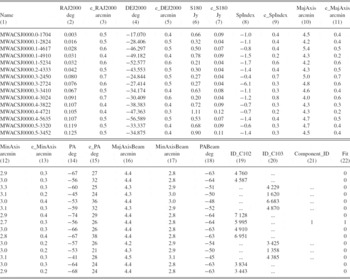
Examples of each method are shown in Figure 15. The fitted spectral indices and 180 MHz flux densities for the components of resolved sources are reported in the catalogue in the same way as for the unresolved sources. As shown in Table 4, a column in the table indicates whether the spectral index was determined by integrating an extended source, or performing a forced measurement.

Figure 15. Examples of measuring extended emission; top: cross-matching extended components; middle: integrating a flux density where the source is comprised of multiple components; bottom: forcing measurements on faint sources. In each case, the 180 MHz image is shown on the left, the 150 MHz image in the middle, and the 119 MHz image on the right. All images are square and measure 21′ on each side. The colour scales are linear and the same for each source; the minimum is always − 0.2Jy beam^{− 1} and the maxima are 3, 1.5 and 0.4 Jy beam^{− 1}, from top to bottom. The white contours are linear at 5σ levels, starting at 4σ; left-to-right, top-to-bottom, the local RMS σ = 100, 60, 42, 71, 47, 30, 54, 30, and 23 mJy beam^{− 1}. The effective PSF is shown as a filled ellipse in the bottom-left corner. (a) The source is detected as a single extended object at all frequencies, so the aegean component fits are cross-matched, and the integrated flux densities fitted to produce S _{180 MHz} and α as for unresolved sources. (b) For multiple-component sources where aegean was unable to detect separate components at the lower frequencies, the components detected at 180 MHz are used to set up peaks from which the 150 and 119 MHz images are flood-filled down to a level of 4σ, shown as a thicker contour. The integrated flux densities of the measurements at all three frequencies are used to fit a spectral index for all of the components resolved and reported at 180 MHz. (c) For those sources which are not well-fit by a Gaussian, and are very close to 5σ at the lower frequencies, we force measurements at the position (indicated by a cross) of the 180 MHz centroid (black ellipse) on the 150 and 120 MHz mosaics. All three flux density measurements are used to fit a spectral index for the components resolved and reported at 180 MHz.

Table 4. Source catalogue (only the first 15 sources are shown) table columns are defined as follows: (1) IAU name hhmm.m+ddmm. (2) RA. (3) Error on RA. (4) Dec. (5) Error on Dec. (6) Integrated flux density at 180 MHz. (7) Error on integrated flux density. (8) Spectral index (α where S _ν∝ν^α). (9) Error on spectral index. (10) Major axis of source. (11) Error on major axis. (12) Minor axis of source. (13) Error on minor axis. (14) Position angle of source. (15) Error on position angle of source. (NB 10, 12 & 14, are as measured in the 180 MHz maps and include convolution with the synthesised beam). (16, 17, 18) Major axis, minor axis and position angle of the PSF at location of source. (19) Source index within Dec − 27 field. (20) Source index within Dec − 47 field. (21) For sources where a multi-component fit was required: the index of the component (NB sources in the overlap region are identified by having non-null values for both 19&20. 19, 20 & 21 can be used to cross-match multiple components. All components will share a value for columns 19 and/or 20 with each component source having a unique value for 21). (22) Type of spectral fit used to determine source spectral index; 0 indicates source fitting at all three frequencies (Figure 15a); 1 indicates flood-fill (Figure 15b); 2 indicates a forced measurement (Figure 15c).

Error measurements for the flux densities of these extended sources were identical to those discussed in Section 3.8, with the fitting error combined in quadrature with the RMS noise. It should be noted, however, that the changing resolution of the instrument at different frequencies, combined with the intrinsic complexity of these sources, mean that the automatically derived spectral indices should be treated with caution. Postage stamps of the extended sources are available on request should the reader wish to perform their own measurements.

4.1 Catalogue reliability and completeness

Recall that all of the source-finding for this survey was performed on the highest-frequency mosaic. For point sources, after source identification, the source was fitted at all other frequencies. If any of these fits failed, the source would be treated as resolved; see Section 3.10 for details. We searched for and identified ten spurious sources in the sidelobes of bright sources by searching the areas around (≈ 100) sources of S > 10 Jy, comparing images at all frequencies, and removed these from the catalogue; the faintest source which produced a spurious sidelobe source was 14 Jy. In typical circumstances away from bright sources, we require that all sources are detectable at 5σ at 180 MHz and well-fitted by a Gaussian in the other bands, so with a Gaussian random background, the chance of any source being spurious is vanishingly small. Our noise is somewhat non-Gaussian due to the presence of undeconvolved source sidelobes, but in the general field, these sidelobes are faint due to our good u, v-coverage, which suppresses sidelobes down to a 10% level even before deconvolution; and the positions of change sidelobe alignments would vary with frequency and thus be unlikely to be detected in every channel. Therefore, we can have an extremely high confidence that all of the sources in the catalogue are real.

The varying detection threshold affects the catalogue completeness for two reasons. More obviously, the variations in the local RMS cause a varying absolute detection limit across the field. In addition, the noise in the map introduces a non-zero probability that a source whose intrinsic flux is > 5σ, has a measured flux < 5σ due to instrumental effects (and vice versa). We therefore present the noise properties of our maps in some detail.

4.1.1 Variations in RMS sensitivity

Figure 4 shows maps of the local RMS of the mosaics rescaled to take into account absolute calibration (with XX and YY combined together for the Dec − 47 scan). This information is summarised in Figure 16.

Figure 16. Cumulative distribution functions of the RMS at 180 MHz for those areas of the map outside of the overlap region for the Dec − 27 scan (black dashed line) and Dec − 47 scan (black dotted line). A subset of data truncated in RA and Dec range is also shown for both scans: Dec − 27 (grey dashed line: 22^h00^m < α < 07^h30^m, − 30° < δ < −20°); Dec − 47 (grey dotted line: 21^h15^m < α < 06^h40^m, − 42° < δ < −52°)

This figure shows that the extremely high RMS regions associated with bright extended sources, particularly near the Galactic plane, account for a small proportion of survey area. Overall, the sensitivity of the survey varies about the median of ~ 40 mJy by less than a factor of two over 80% of the survey area, a variation in sensitivity comparable with the VLSS (cf. Cohen et al. Reference Cohen, Lane, Cotton, Kassim, Lazio, Perley, Condon and Erickson2007, Figure 7).

The RMS in the Dec − 27 and Dec − 47 mosaics are reasonably comparable, though the Dec − 47 mosaic has a somewhat lower RMS, particularly for regions below the median. We ascribe this to a better phase calibration for the Dec − 47 data, as a brighter phase calibrator was used. The RMS becomes only marginally worse towards the edge of the primary beam in the Dec − 47 mosaic, however it becomes significantly worse towards the edge of the primary beam in the Dec − 27 mosaic. This is because the sky rotates more quickly through the primary beam closer to the celestial equator.

Figure 17 shows the histogram of flux density values across a significant proportion of each mosaic. When calculated over a wide area, the RMS for the two maps agrees to ~ 10%; 90% of the surveyed area has an RMS lower than 50 mJy, except for the very northern edge.

Figure 17. Histogram of the pixel brightness of the 180 MHz maps (P(D)). RA and Dec ranges are 22^h00^m < α < 07^h30^m, − 30° < δ < −20° (approx 1 300 square degrees) for the Dec − 27 mosaic (top) and 21^h15^m < α < 06^h40^m, − 42° < δ < −52° (approx 1 000 square degrees) for the Dec − 47 mosaic (bottom). The RMS for each pixel distribution (determined via the semi-interhexile range) is 0.035 Jy beam^{− 1} and 0.029 Jy beam^{− 1} respectively. The dashed line is a gaussian curve with this RMS, centred on the median flux density (− 2.4 mJy beam^{− 1} and − 3.2 mJy beam^{− 1} respectively).

4.2 Fornax A

Fornax A is a nearby (z ≈ 0.006) radio galaxy, situated in the Fornax cluster of galaxies. It comprises two large lobes extending NNW and SSE 20 arcmin (≈ 200 kpc) from the lenticular galaxy NGC 1316, at RA = 03^h 22^m 41^s.789 Dec = − 37°12′ 29.′′52. On scales ≳ 20′ , structure is not sampled by MWACS, so we cannot measure the integrated flux density for this object, only set lower limits. This under-sampling also causes deconvolution errors across our mosaics, resulting in increased noise levels around the Fornax A region.

Using blobcat to flood-fill the entire region down to a 4σ level and measure the integrated flux density, we set lower limits across the entirety of Fornax A at 786 ± 39, 668 ± 33, and 514 ± 26 Jy at 120, 150, and 180 MHz, respectively; these are consistent with the values measured by Bernardi et al. (Reference Bernardi2013) and McKinley et al. (Reference McKinley2014). An image of the radio galaxy at the highest MWACS resolution is shown in Figure 18.

Figure 18. Fornax A at 180 MHz; contours are linear at 10% levels from the peak brightness of 16.75 Jy beam^{− 1}. The synthesised beam is shown as an open ellipse at the bottom-left of the image, with dimensions 4.22 arcmin × 2.85 arcmin, position angle − 53.°8. The RMS of this image is 92 mJy.