


Introduction
Although southern European countries still hold vast areas of agro-steppes, the current multifactorial changes at the landscape level, induced both by agricultural intensification and abandonment, combined with increasingly frequent construction of infrastructure, such as highways, railroads, dams, power lines and urban sprawl (e.g. Morales et al. Reference Morales, Mañosa and Camprodon2005, Martínez-Abraín et al. 2009) are causing large-scale habitat modification and fragmentation. These changes may imply serious risks for endangered species living in these areas. The Little Bustard Tetrax tetrax is a bird that lives in natural steppes and in extensive agricultural landscapes and it has been decreasing and disappearing from several countries (Iñigo and Borov Reference Iñigo and Borov2010, Silva et al. Reference Silva, Estanque, Moreira and Palmeirim2014a). The species has a fragmented range encompassing south-western and south-eastern Europe and Central Asia (Iñigo and Borov Reference Iñigo and Borov2010, Silva et al. Reference Silva, Estanque, Moreira and Palmeirim2014a). It is considered Near Threatened (IUCN 2008) and a conservation priority species under the European Bird Directive (2009/147/CE). Several studies indicate that agricultural intensification and landscape structural changes are the main reasons for its decline (Martínez and Tapia, Reference Martínez and Tapia2002, Traba et al., Reference Traba, Morales, de la Morena, Delgado and Krištín2008, Bretagnolle et al. Reference Bretagnolle, Villers, Denonfoux, Cornulier, Inchausti and Badenhausser2011). Most works concerning Little Bustard focus on the agricultural patchwork configuration, field characteristics/management and species bio-ecology (Traba et al. Reference Traba, Morales, de la Morena, Delgado and Krištín2008, Bretagnolle et al. Reference Bretagnolle, Villers, Denonfoux, Cornulier, Inchausti and Badenhausser2011, Faria et al. Reference Faria, Rabaça and Morales2012, Moreira et al. Reference Moreira, Silva, Estanque, Palmeirim, Lecoq, Pinto, Leitão, Alonso, Pedroso, Santos, Catry, Silva, Henrqiues and Delgado2012, Tarjuelo et al. Reference Tarjuelo, Delgado, Bota, Morales, Traba, Ponjoan, Hervás and Mañosa2013) but few address mortality and exclusion/barrier effects associated with utility corridors such as roads and overhead power lines (e.g. Silva et al. Reference Silva, Santos, Queirós, Leitão, Moreira, Pinto, Lecoq and Cabral2010, Reference Silva, Palmeirim, Alcazar, Correia, Delgado and Moreira2014b). Actually the combined influence of overhead power lines, road networks and agricultural changes on the density of Little Bustard breeding populations was, to the best of our knowledge, only assessed by Silva et al. (Reference Silva, Santos, Queirós, Leitão, Moreira, Pinto, Lecoq and Cabral2010). That work depicts a useful methodology to predict changes in Little Bustard density for specific locations within a site (areas holding important populations) and considers dynamic changes in the surrounding habitats. Nevertheless, that study was not able to expand and/or project the explicit spatio-temporal responses to the entire site (Silva et al. Reference Silva, Santos, Queirós, Leitão, Moreira, Pinto, Lecoq and Cabral2010, Santos et al. Reference Santos, Bastos and Cabral2013). When local processes such as land use changes become so significant as to affect species dynamics, spatially explicit methods are proposed, providing powerful ways to link fine-scale changes to coarse-scale dynamics (Liebhold and Gurevitch Reference Liebhold and Gurevitch2002, Chen et al. Reference Chen, Han, Ye and Li2011, Santos et al. Reference Santos, Bastos and Cabral2013). This is particularly relevant for the Little Bustard that depends on the presence of specific habitats within a complex and highly dynamic mosaic of agro-ecosystems (Delgado et al. Reference Delgado, Morales, Traba and Garcia de la Morena2009).
In support of technical and political decisions, modelling can be very useful as a research tool to predict the outcome of alternative scenarios, guiding current management options from expected future targets and simulating conditions that are difficult or impossible to understand otherwise (e.g. Santos et al. Reference Santos, Bastos and Cabral2013). The Stochastic Dynamic Methodology (StDM) has been developed as a sequential modelling process to predict the ecological status of changing ecosystems, from which management strategies can be designed (Santos and Cabral Reference Santos and Cabral2004). This recent research is based on the premise that general statistical patterns of ecological phenomena are emergent indices of complex ecological processes (Santos and Cabral Reference Santos and Cabral2004). The Stochastic Dynamic Methodology (StDM) combines statistical and dynamic modelling with geostatistical techniques to address complex spatially-explicit emergent problems, from the individual habitat patch to the whole landscape context (Santos et al. Reference Santos, Bastos and Cabral2013). While the parameters of the dynamic model can be calibrated directly from knowledge of ecosystem characteristics and bibliographic information (ecologically driven), others, namely holistic parameters, have to be estimated using statistical algorithms, i.e. stochastically generated (black-box). The stochastically derived parameters, if supported by a database that includes relevant gradients, represent effective conceptual representations of spatial and temporal ecosystem properties and might be used for simulation or prediction, assuming that ecosystem conditions remain comparable. The StDM is initiated by the analysis of landscape and habitat composition, which defines the suitable parameters that contextualize the physical and biotic descriptors at the study unit level. This procedure involves the use of robust information and theoretic approaches based on generalized linear models (Nelder and Wedderburn Reference Nelder and Wedderburn1972) in order to establish the interaction criteria between the construction of the dynamic model (Ford Reference Ford1999) and the resulting stochastic dynamic simulations for each study unit (Bastos et al. Reference Bastos, Santos, Ramos, Vicente, Guerra, Alonso, Honrado, Ceia, Timóteo and Cabral2012, Santos et al. Reference Santos, Bastos and Cabral2013). These simulations, when projected into a geographic space (e.g. Johnston Reference Johnston1998) and submitted to an appropriate geostatistical interpolation (Urban Reference Urban2006), create an integrative picture, in space and time, of the responses to the gradients of habitat changes, namely considering management options and species responses. When applied as a multi-scale approach to address the effects of drivers on relevant indicators, the StDM’s spatially explicit outputs (Bastos et al. Reference Bastos, Santos, Ramos, Vicente, Guerra, Alonso, Honrado, Ceia, Timóteo and Cabral2012, Santos et al. Reference Santos, Bastos and Cabral2013) can be interpreted both locally and regionally, considering stochastic phenomena that characterise ecological processes. The StDM framework has been successfully tested in several types of ecosystems affected by gradients of change (Santos et al. Reference Santos, Bastos, Travassos, Bessa, Repas and Cabral2010, Reference Santos, Freitas, Crespí, Hughes and Cabral2011, Carvalho et al. Reference Carvalho, Horta, Raposeira, Santos, Luís and Cabral2013, Fernandes et al. Reference Fernandes, Cabral, Crespí, Hughes and Santos2013) including wildlife conservation (Silva et al. Reference Silva, Santos, Queirós, Leitão, Moreira, Pinto, Lecoq and Cabral2010, Bastos et al. Reference Bastos, Santos, Ramos, Vicente, Guerra, Alonso, Honrado, Ceia, Timóteo and Cabral2012).
In this way, the objectives of the present work were: (1) modelling site-specific spatio-temporal changes in the landscape, specifically agriculture conversion, linear infrastructure installation (such as roads and overhead power lines) and the combination of both stressors; (2) uncovering the effects of these changes on particular Little Bustard breeding populations, whose spatially explicit distribution patterns are the basis of the ecological assessments; (3) supporting site management and policy decisions by creating a tool informing the consequences of alternative landscape scenarios on the species distribution and abundances; and (4) comparing the StDM framework with analogous methodologies for assessing impacts of landscape changes on threatened species.
Material and methods
Study area and Little Bustard counts
The StDM model construction was supported by existing databases related to the campaigns carried out during the national breeding census, between 2003 and 2006, in the Alentejo region (Project LIFE02NAT/P/8476: Conservation of the Little Bustard in Alentejo), which holds the most important populations of the species in Portugal (http://life-sisao.spea.pt/pt/). Since females and non-breeding males are not conspicuous enough to be detected in workable numbers, Little Bustard censuses were based on breeding male estimates derived from 868 survey points performed at 31 sites (Figure 1). A second survey programme with 697 survey points was carried out during 2010 in 22 of these sites, and these data used to assess the StDM model performance. Census details are provided Appendix S1 in the online supplementary material. Spatial correlation of Little Bustard male abundance was assessed by Moran’s I, by comparing values found at all pairs of points in the given distance class (Moran Reference Moran1950).

Figure 1. (A) Location of the Alentejo region in southern Portugal and (B) the spatial distribution of the sites (white shapes) in the study area.
StDM methodology
Stochastic Dynamic Methodology (StDM) is a mechanistic framework for understanding ecological processes based on statistical parameter estimation methods (Santos and Cabral Reference Santos and Cabral2004, Santos et al. Reference Santos, Freitas, Crespí, Hughes and Cabral2011, Reference Santos, Bastos and Cabral2013). This methodology combines both modelling paradigms, black-box and ecologically driven models within the same application. The basic unit of a StDM model is a state variable based on the relationships detected in the statistical analysis, described by difference equations (the discrete parallel to differential equations, where we use old values from the system to calculate new ones). Generically, the response variables of the statistical model correspond to the ecological consequences or state variables under study and the explanatory variables are the principal environmental factors or drivers considered. Therefore, StDM models base the inflows and outflows of these state variables on constants and coefficients of the statistical model (Appendix S2.1). Nevertheless, since the previous statistical test output is static, one of the central requirements of StDM is that the dataset used for parametrising the stochastic component includes relevant environmental gradients (Santos and Cabral Reference Santos and Cabral2004), allowing more realism, as the respective parameters are being considered with regard to their embedding in time and space (Santos et al. Reference Santos, Bastos and Cabral2013). The partial regression coefficients represent the global influence of the environmental variables selected that are of significance on several complex ecological processes. Yet the latter are not included explicitly in the model, but taken into consideration within the “data-space” of the environmental gradients monitored in changed ecosystems.
The spatially explicit StDM framework
General overview
The proposed Spatially Explicit StDM framework is a sequential process for detecting the influence of spatio-temporal changes in the functioning of selected elements of ecosystems, as depicted in Figure 2 (details in Appendix S2.2).

Figure 2. The Spatially Explicit StDM framework for forecasting changes in Little Bustard abundance and distribution as a response to local drivers: (A) analyses of landscape in each survey point surrounding area; (B) the statistical analysis to determine the convenient parameters that capture the influence of the land use/cover and infrastructure characteristics on the species’ response at the survey point level; (C) the construction of the stochastic dynamic model for simulating abundance trends at the point level; (D) site specific projection of the resultant stochastic dynamic point simulations into a geographic plane; (E) site specific geostatistical chrono-sequential interpolations for creating interactive and integrative pictures.
Land use/cover mapping and habitat classes
Land use/cover of every survey point (within a circular buffer of 250 m; Appendix S1) was characterised (Figure 2A) using a GIS database (Corine Land Cover 2006; Caetano et al. Reference Caetano, Nunes and Nunes2009). Land use/cover was grouped in eight classes, Rainfed, Artificial Surfaces, Irrigated Crops, Permanent Crops, Heterogeneous Agriculture, Forests, Water bodies and Other (Table 1). Additional information was collected for calculating infrastructure attributes associated with overhead power lines and road network: Line Length, Roads Length and Line Distance (Table 1). The spatial analyses were carried out using ArcGIS® 10.1 Geographic Information System software (Esri 2013) and SAM (Rangel et al. Reference Rangel, Diniz-Filho and Bini2010).
Table 1. List of the variables considered in the StDM model construction

Statistical analyses
The StDM dynamic model construction (Figure 2C) was preceded by a statistical procedure (Figure 2B) for parameter estimation, testing relationships between response and explanatory variables (Santos and Cabral Reference Santos and Cabral2004). The response variable corresponds to Little Bustard male abundance and the explanatory variables are expressed by the area occupied by each habitat class and linear infrastructures associated that characterised each point (Silva et al. Reference Silva, Santos, Queirós, Leitão, Moreira, Pinto, Lecoq and Cabral2010). In order to avoid multicollinearity, the 10 predictors selected were tested for pairwise correlation using Spearman’s rho correlation coefficient and only predictors with correlation lower than 0.7 (Elith et al. Reference Elith, Graham, Anderson, Ferrier, Dudik, Guisan, Hijmans, Huettmann, Leathwick, Lehmann, Li, Lohmann, Loiselle, Manion, Moritz, Nakamura, Nakazawa, Overton, Peterson, Phillips, Richardson, Scachetti-Pereira, Schapire, Soberon, Williams, Wisz and Zimmermann2006, Wisz and Guisan Reference Wisz and Guisan2009) and Generalized Variance Inflation Factor lower than 5 were considered (Neter et al. Reference Neter, Kutner, Nachtshei and Wasserma1996). A generalized linear model (GLM) with a log-link function to fit the model (count data with an approximate Poisson distribution; O’Hara and Kotze, Reference O’Hara and Kotze2010) was used so that the effect of each explanatory variable in the presence of all others could be examined prior to the dynamic model construction (Figure 2B). We assessed the fit of each candidate model using the Akaike Information Criterion (AIC) value (Akaike Reference Akaike1974, Hurvich and Tsai Reference Hurvich and Tsai1989), by comparing all possible combinations using the Akaike weights (AICwi; Anderson et al. Reference Anderson, Burnham and Thompson2000). In order to reduce complexity, we selected the “best model” supported by the data (lower AIC and higher adjusted R2; Santos et al. Reference Santos, Freitas, Crespí, Hughes and Cabral2011). All statistical analyses (Appendix S2.3) were carried out using Genstat statistical software (version 13.0, VSN International) and SAM (Rangel et al. Reference Rangel, Diniz-Filho and Bini2010).
Conceptualisation of the dynamic model
Significant partial regression coefficients were used to construct a stochastic dynamic model (e.g. Santos and Cabral Reference Santos and Cabral2004, Santos et al. Reference Santos, Bastos and Cabral2013) for estimating Little Bustard occurrence and abundance in changing habitats (Figure 2B). In a holistic perspective, the partial regression coefficients represent the influence of the habitat variables selected that are of significant importance on several complex ecological processes (Santos and Cabral Reference Santos and Cabral2004) and are related to Little Bustard occurrence. We used the software STELLA (version 10.1., Isee Systems, Inc., http://www.iseesystems.com) for the dynamic model development. The model was also constructed to automatically receive each point land use/cover and infrastructural variables for different periods, calculating the rates of change used for modelling each point landscape dynamics.
Converting dynamic simulations in spatially explicit dynamic projections
To create the spatial dynamic projections for each site, the dynamic simulations by point were achieved considering the respective trends in land use/cover and linear infrastructure. Using this information the StDM model was able to estimate the respective abundance of the Little Bustard for each point in the periods considered (Figure 2D). The spatial representation of multiple StDM simulations enabled the creation of geographical projections of land use/cover, linear infrastructure and Little Bustard densities for each site (Fig. 2E, Appendix S2.4) (Cressie and Ver Hoef Reference Cressie, Ver Hoef, Goodchild, Parks and Steyaert1993, Walker et al. Reference Walker, Balling, Briggs, Katti, Warren and Wentz2008, Dormann Reference Dormann, Jopp, Reuter and Breckling2011, Sherman Reference Sherman2011, Zhang and Murayama Reference Zhang and Murayama2000).
The framework simulations were analysed facing realistic scenarios of change, in terms of land use and/or infrastructural alterations: scenario 1 associated with actual infrastructure developments and small changes in land use/cover that have occurred in the site within the study region called “Cuba”; scenario 2 related to no infrastructure developments but with large transformations in land uses/cover that have occurred in the site within the study region called “Airoso”, mostly related with irrigation and agriculture intensification supplied by the increasing water availability from the recently built Alqueva Dam (Costa et al. Reference Costa, Moors and Fraser2011); scenario 3, applied in the “Airoso” site and combining the actual land use changes with possible infrastructure developments. In order to perceive changes in the landscape and compare Little Bustard densities and distribution, three time steps of the dynamic simulations were selected from which the respective spatial projections were depicted (Figures 2D, 2E).
Spatially explicit StDM framework performance
For assessing regional performance for the Alentejo, a set of independent data was used to compare the simulated populations with real estimated populations (22 sites monitored in 2010). Results of the average population estimates for these sites were compared with the respective expected values from our spatially explicit simulations, using Model II regression analyses (Standardized Major Axis regression-SMA using the software SMATR 3.0; Warton et al. Reference Warton, Duursma, Falster and Taskinen2012). The 95% confidence limits for the intercept and the slope of the regression were determined for each analysis to assess the proximity of the produced simulations in relation to the respective estimated values (Sokal and Rohlf Reference Sokal and Rohlf1995). The spatially explicit simulations were considered with regional accuracy (considering all sites from the Alentejo region) when (1) a statistically significant correlation occurred between both sets of data (simulated populations per site versus estimated populations per site); (2) the intercept of the common regression line was not statistically significantly different from 0 and; (3) the slope of the common regression line was not statistically significantly different from 1 (Sokal and Rohlf Reference Sokal and Rohlf1995, Warton et al. Reference Warton, Duursma, Falster and Taskinen2012). Complementary to the previous regional performance assessment, differences between each point simulated abundances and estimated abundances (grouped by site) were compared to assess local performances using the Wilcoxon signed rank test (Wilcoxon Reference Wilcoxon1945). The simulations were considered with local accuracy if the simulated abundances and the estimated abundances were not different from each other (statistically non-significant differences between the simulated and estimated values).
Results
Effects of environmental variables on the abundance of Little Bustard males
A total of 11 independent variables (Table 1) were considered in the GLM analysis to test any possible correlation between the Little Bustard’s (male) abundance and the habitat variables of the data used in the StDM model construction. With regard to significant habitat variables, the abundance was found to be positively related with the area occupied in each point by Rainfed (rain-fed cereals, fallow and pastures) and negatively related to the area of Water bodies (reservoirs), Forests (natural and planted), Line Length (metres of overhead high tension power line) and Roads Length (the metres of paved road) in each point (AIC = 1,411. 7; df = 6; Adj. R2 = 8.31; F = 39.62; P < 0.001; Appendix S3). GLM residuals seem to show the same pattern of the raw data, i.e. positive autocorrelation at shorter distances and a mostly negative autocorrelation at longer distances (Appendix S4).
Dynamic model conceptualisation
The dynamic model was constructed to simulate land use changes and infrastructural developments, using the actual and predicted areas/lengths occupied by land use / cover and infrastructure: rates were calculated using historical information for each point in each site (Caetano et al. Reference Caetano, Nunes and Nunes2009). The GLM significant partial regression coefficients were used to estimate Little Bustard occurrence and abundance under the influence of land use/cover and infrastructural changes (Santos et al. Reference Santos, Bastos and Cabral2013). The original conceptual diagram of the overall model and full explanation of processes, parameters and equations included in the model construction are shown in Appendices S2, S5, S6.
Spatially explicit dynamic scenarios
Scenario 1
The interpolated spatio-temporal simulations, incorporating the spatial autocorrelation in the kriging procedure, of the landscape changes that have occurred from the years 2003 to 2010 in the site of “Cuba” and the respective interpolated Little Bustard responses, expressed in densities (number of males per 100 ha), are shown in Figure 3 (semi-variograms and Moran’s I are depicted in Appendix S7). The importance of the areas occupied by Rainfed land use, a main road crossing the southeast and the installation of an overhead transmission power line in 2004, in the extreme north are the core variables depicted (Figure 3A). The interpolated influence of these multifactorial changes in the density of the Little Bustard is shown in Figure 3B: higher densities seem to be associated with areas away from the main road and, with the construction of the overhead power line, of both infrastructures and dominated by Rainfed land use. Overall the population of this site was predicted to have decreased by 5% from 2003 to 2010 in response to the landscape changes associated with the construction of the overhead power line and a small decrease in the Rainfed area (Appendix S8).

Figure 3. (A) Spatial representation of changes in the land use/cover and infrastructure for scenario 1 and (B) the respective Little Bustard responses, expressed in densities (applied to the “Cuba” site). The main change is associated with the installation in 2004 (t = 3) of an overhead power line. Only Rainfed land use/cover is represented considering that all other land use/cover values are below 25% of representativeness. Little Bustard densities were calculated with a continuous distribution function based on a simple kriging and its temporal variation from t = 1 to t = 8. The distribution area was calculated based in the aggregation of the point referenced data.
Scenario 2
In “Airoso” site the landscape changes were mostly related to the substitution of crops. The interpolated spatio-temporal simulations, incorporating the spatial autocorrelation in the kriging procedure, of the landscape changes, from the years 2004 to 2010 and the respective interpolated Little Bustard density responses are shown in Figure 4 (semi-variograms and Moran’s I are in Appendix S7). The reduction in the areas of Rainfed land use/cover, substituted by Permanent crops, through a conversion to olive orchards (Figures 4A and 4B) was predicted to have caused changes in the distribution and a general decline in the population (Figure 4C). In fact in the north of the site, the population collapsed in response to the changes that occurred and only the southern fringes still hold significant densities. Overall, the population of the “Airoso” site was predicted to have decreased by 45% in response to the combination of land use changes described (Appendix S9).

Figure 4. Spatial representation of the main changes in land use/cover for scenario 2: (A) the decrease in the area occupied by Rainfed, (B) the concomitant increase in the area dominated by Permanent crops (olive orchards), and (C) the respective Little Bustard responses, expressed in densities (applied to the “Airoso” site). Little Bustard densities were calculated considering a continuous distribution function based on a simple kriging and its temporal variation from t = 1 to t = 7. The distribution area was calculated based in the aggregation of the point referenced data.
Scenario 3
The interpolated spatio-temporal simulations, combining land use changes (identical to scenario 2) with the possible construction of a road in the south and the installation of an overhead transmission power line crossing the “Airoso” site during 2008 and the respective interpolated Little Bustard density responses are depicted in Figure 5. These changes could intensify the scenario 2 general decline in the population (Figure 4C versus Figure 5C), namely in the southern fringes. Overall, the population of the “Airoso” site could have decreased by 56% (an extra 11% decline, compared to scenario 2) in response to the combination of stressors described (Appendix S10).

Figure 5. Spatial representation of the main changes in the land use/cover and infrastructures for scenario 3: (A) the decrease in area occupied by Rainfed and the installation of power lines and a road in 2008, (B) the concomitant increase of the area dominated by Permanent crops (olive orchards), and (C) the respective Little Bustard responses, expressed in densities (applied to the “Airoso” site). Little Bustard densities were calculated considering a continuous distribution function based on a simple kriging and its temporal variation from t = 1 to t = 7. The distribution area was calculated based on aggregation of the point referenced data.
Spatially explicit StDM framework performance
The results of the performance analysis, based on the confrontation between simulated and estimated values for 22 independent sites (not used to construct the model), expressed in the respective populations are shown in Figure 6. Despite the non-statistical validation of our regional estimates (n = 22; R2= 0.808; T = -4.451; F = 136.554; P < 0.001; Appendix S11), we could easily recognise the consistent patterns in the spatially explicit outputs, although sometimes underestimated or overestimated in identifying the population of these sites (Figure 6). Moreover, 66% of the most important sites (Silva and Pinto Reference Silva and Pinto2006), with estimated populations of 100 or more males were predicted by the framework to attain populations above 100 (Figure 6). Concerning our local performance assessment, in 55% of sites (12 out of 22) the confrontation between the interpolated abundances simulated and estimated by point was not statistically significantly different (Table 2).

Figure 6. Comparisons between simulated and estimated male population sizes by site and associated standard errors (error bars). Dashed line separates sites with more than 100 males.
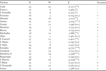
Table 2. Results of the Wilcoxon test for comparisons between simulated and estimated males abundances by survey point (grouped by site). Number of points by site (N), the Wilcoxon value (W), verification of differences using Z-value (Z) and significance level (*** - P < 0.001, ** - P < 0.01, * - P < 0.05, ns – non significant). The last column summarizes the sites that were accurately predicted “+” and inaccurately predicted“−”.
Discussion
Habitats, infrastructure and bird density
The StDM spatially explicit patterns simulated are in agreement with previous studies showing higher densities of the Little Bustard in areas of extensive fallow/pastures and cereal (e.g. Silva et al. Reference Silva, Faria and Catry2007, Moreira et al. Reference Moreira, Silva, Estanque, Palmeirim, Lecoq, Pinto, Leitão, Alonso, Pedroso, Santos, Catry, Silva, Henrqiues and Delgado2012). The predicted absences and/or low densities are mainly related to the dominance of other land uses, particularly forests, permanent crops and intensive agriculture, which are mostly unsuitable habitats for the species (Garcia et al. Reference Garcia, Suárez-Seoane, Miguélez, Osborne and Zumalacárregui2007, Delgado et al. Reference Delgado, Morales, Traba and Garcia de la Morena2009, Silva et al. Reference Silva, Estanque, Moreira and Palmeirim2014a). In fact, the population size and spatial distribution throughout simulations seemed to be greatly influenced by the dynamics of the land use/cover, stressing the importance of the landscape patchwork layout for conservation of the species (Osborne and Suárez-Seoane Reference Osborne and Suárez-Seoane2006).
Nevertheless, the progressive development of infrastructure, such as roads and overhead transmission power lines, even in areas of suitable habitat, contributes to the deterioration in the ecological conditions in such places, with negative consequences for the species’ distribution and abundance. Our results suggesting that infrastructure can have an additional negative impact, namely associated with an exclusion effect, on Little Bustard breeding populations and that this impact is more evident close to the infrastructure are in agreement with other work on similar species (e.g. Benítez-López et al. Reference Benítez-López, Alkemade and Verweij2010). The most commonly reported impacts of infrastructure include habitat loss, intrusion of edge effects in natural areas, isolation of populations, barrier effects, road mortality, collisions and increased human access (Janss et al. Reference Janss2000, Benítez-López et al. Reference Benítez-López, Alkemade and Verweij2010, Santos et al. Reference Santos, Bastos, Travassos, Bessa, Repas and Cabral2010, Silva et al. Reference Silva, Santos, Queirós, Leitão, Moreira, Pinto, Lecoq and Cabral2010). Several works also report increasing levels of predation by birds of prey near infrastructure, reducing habitat quality and the abundance of many prey species (e.g. Lambertucci et al. Reference Lambertucci, Speziale, Rogers and Morales2009). Overall, the StDM framework outputs suggest that the sustainability of each site’s reproductive population may be guaranteed by combining suitable land use with the absence or distant installation of linear infrastructure such as roads and overhead power lines. Although the patterns of our model are clear, we would like to emphasize that these only represent a partial estimate of the actual combined effect of landscape on Little Bustard breeding populations. Therefore, we highlight the importance of broadening the analysis to other parts of the year, namely winter (Silva et al. Reference Silva, Pinto and Palmeirim2004) when habitat selection by the species can be different and using complementary information, such as mortality or landscape genetics, to assess real impacts. These developments would add to the current holistic model/framework presented, contributing to an integrative methodology that would provide a more accurate estimate of the effects of infrastructure development and landscape changes on Little Bustard populations.
Methodology usefulness
Ecologists classify most quantitative models into correlative models (black-box models: Species Distribution Models, Maxent and others) and ecologically driven models (System Dynamics, Agent Based, Discrete-Event and others) (Guisan and Zimmermann Reference Guisan and Zimmermann2000, Jørgensen Reference Jørgensen2008). Black-box models, although used to simplify the modelling protocol in ecological processes, are considered unable to describe, in a comprehensible way, the structural changes when ecosystem conditions are changing substantially (e.g. Perry and Millington Reference Perry and Millington2008). In fact, in holistic correlative approaches, many details are not considered, such as individual variability, adaptation, local idiosyncrasies, and highly dynamic ecological phenomena. Although this simplification enables the understanding of whole-system processes such as resilience, resistance, persistence, regulation, and density dependence, it is difficult to follow at other scales, namely when local properties are crucial to the system’s behaviour.
On the other hand, the strength of ecologically driven models lies in their ability to take into account the individual/systemic and evolving nature of inter-related activities, showing the interactions between principal drivers (Chen et al. Reference Chen, Han, Ye and Li2011). Although ecologically driven models are usually data-intensive and frequently over-parameterized, many scientists consider them useful in a wide variety of applications related to ecosystem functioning (e.g. Jørgensen Reference Jørgensen2008). Furthermore, modellers or users of these models should address the issue of the applicability of the models in data-poor conditions, especially when multitudes of field parameters, which are necessary for empiric model calibration, are not available (Santos et al. 2013, Reference Santos, Bastos, Vicente, Berger, Filho, Rodrigues, Alonso, Guerra, Martins, Honrado, Cabral and Canning-ClodeSantos et al. in press). Actually, in a reductionist analytical perspective, parameter estimation is often the weakest point in modelling (van Nes and Scheffer Reference van Nes and Scheffer2005). Determining the appropriate values of the parameters entered in the model is one of the most critical and challenging parts of model building (Santos et al. Reference Santos, Bastos and Cabral2013).
The main objective of applying the StDM methodology is to minimise problems in model creation such as parameterisation, model complexity and choice of variables (Santos et al. Reference Santos, Freitas, Crespí, Hughes and Cabral2011). The StDM incorporates a number of particularities when compared to the usual ecological dynamic modelling approaches. The first and probably the most important difference is calculation of the parameters that result from statistical estimation. Therefore, the sensitivity analysis routine, considered crucial in standard dynamic modelling, is not an imperative for StDM parameter estimation and dynamic model testing (Santos et al. Reference Santos, Bastos and Cabral2013). This modelling tool has emerged from the idea of the so-called hybrid models (Chen et al. Reference Chen, Han, Ye and Li2011): modelling species distributions on the basis of large-scale holistic relationships while at the same time considering the most important processes. This is one of the major advantages of StDM models (Santos et al. Reference Santos, Bastos and Cabral2013): combining different approaches and enabling information transfer at a local scale, facilitating a better understanding of ecosystem dynamics, and leading to emergence and similar system characteristics.
The results obtained also show that space-for-time information in an StDM application can overcome problems associated with chrono-sequential information (Santos and Cabral Reference Santos and Cabral2004). The fact that studies in environmental change and community dynamics require regularly updated information further compounds the problem of data availability (Santos et al. Reference Santos, Bastos and Cabral2013). The identified spatial autocorrelation patterns in the Little Bustard distribution, probably associated with the males’ lekking behaviour, were not solved in the GLM but were incorporated in the final spatio-temporal StDM simulations. Kriging, which accounts for spatial autocorrelation based on a variogram, provided a way to estimate a spatial random field at unobserved locations (Urban Reference Urban2006). This technique computes the value of interest at an unknown point as a weighted average, defined by the variogram model of the sampled neighbours (Urban Reference Urban2006). The option of using this technique following the GLM to adjust autocorrelation, instead of other spatial models (generalized least squares, geographically weighted regressions, among others) (Rangel et al. Reference Rangel, Diniz-Filho and Bini2010) which correct autocorrelation and create new parameters for the dynamic model, was related to work with a more parsimonious StDM model, while incorporating spatial autocorrelation as an ecological factor affecting species abundance and distribution.
Implications for conservation
Regarding a priority species depending on traditional agriculture and occurring in areas which are mostly classified under the European protected area network (Natura 2000, special protection areas and others) this study highlights the conflicts between conservation efforts, agricultural conversion and/or infrastructure development such as utility corridors. Therefore, there is an increased need for management policies in the European network of protected areas to take appropriate action to avoid a deterioration in habitat and other disturbance affecting birds (Directive 2009/147/EC). In the present work, the combined effects of roads and overhead transmission lines did not per se imply a significant decrease in the overall population size but caused changes in the use of space by the species, contributing to a higher aggregation, which might in turn lead to higher vulnerability due to population and environmental stochasticity (Torres et al. Reference Torres, Palacín, Seoane and Alonso2011). In other words, distance from linear infrastructure is an important variable even in areas dominated by high quality breeding habitat (fallows, non-irrigated cereals and pastures). On the other hand, Little Bustard density decreases associated with agriculture conversion might reduce dramatically the breeding populations in areas considered crucial for nature conservation. A defensible strategy for conservation can be created, and most reliably will involve long-term maintenance of agro-steppe areas and management, using agri-environmental measures, combined with a limited and distant road and overhead power line network. The challenge will be for local and national authorities, jointly with farmers and linear infrastructure stakeholders, to outline the main corridors for these utility infrastructures that avoid priority conservation sites.
Conclusion
Our results contribute to increasing the knowledge of the responses of Little Bustard populations to the combined effects of utility corridors in a dynamic context of agricultural changes, quantifying some of the negative effects that should be considered when planning and evaluating alternative infrastructure developments and landscape planning. Specifically, our framework can be used to demonstrate and support decisions such as the implementation of agri-environment schemes and infrastructure location, improving the current situation where results of previous studies on ecological directives or estimated impacts are barely taken into account (Roedenbeck et al. Reference Roedenbeck, Fahrig, Findlay, Houlahan, Jaeger, Klar, Kramer-Schadt and van der Grift2007, Stoate et al. Reference Stoate, Báldi, Beja, Boatman, Herzon, Van Doorn, de Snoo, Rakosy and Ramwell2009).
The effective implementation of the Spatially Explicit StDM framework is very recent (Bastos et al. Reference Bastos, Santos, Ramos, Vicente, Guerra, Alonso, Honrado, Ceia, Timóteo and Cabral2012, Santos et al. Reference Santos, Bastos and Cabral2013). Although conceptually simpler and more intuitive than other modelling methodologies such as Artificial Intelligence (Džeroski et al. Reference Džeroski, Grbovic, Walley and Kompare1997), the modelling framework can predict ecological trends, including relevant temporal and spatial gradients of stochastic environmental characteristics. It provides accessible explanations for underlying associations between variables based on conventional statistical methods that allow a more direct development of testable hypotheses. Additionally, the development of ecosystem change assessment methodologies must take into account the application’s viability and if the results can be applied to other areas of interest (Andreasen et al. Reference Andreasen, O’Neill, Noss and Slosser2001). The proposed methodology and model was parametrised for the Alentejo region (south-west Iberia) and can be easily adjusted or adapted to other species, other sites in the region and eventually to similar regions of Iberia.
This type of modelling may provide a basis for decision-making regarding permitting and mitigating prior to construction of infrastructure and/or land use changes, when few other tools are available for making such decisions. The work also provides valuable information to assess the negative impact of existing infrastructure as well as allowing the recognition of locations that should be avoided when constructing new developments. Overall, our approach can underpin landscape management and policy decisions in agricultural landscapes and assure ecosystem services/conservation of wildlife in the face of ongoing environmental changes.
Supplementary material
To view supplementary material for this article, please visit https://doi.org/10.1017/S0959270915000258
Acknowledgements
The authors are indebted to all who carried out the Little Bustard surveys in 2003–2006 and 2010, namely A. Cavaco, A. Delgado, B. Estanque, C. Carrapato, C. Cruz, C. Conde, D. Leitão, E. Santos, G. Gaspar, I. Henriques, I. Alonso, J. Baptista, N. Sequeira, P. Rocha, R. Alcazar, R. Pedroso. Special thanks are addressed to Robert Sauvé for the English revision of our manuscript. The 2003–2006 monitoring programme was part of the project LIFE02NAT/P/8476 “Project Tetrax: the conservation of the Little Bustard in the Alentejo”. Regina Bessa was financially supported by a scholarship of the Laboratory of Applied Ecology of the University of Trás-os-Montes e Alto Douro. João Paulo Silva was funded by grant SFRH/BPD/72311/2010 from Fundação para a Ciência e Tecnologia.


