


Introduction
Group testing is becoming increasingly popular because it can substantially reduce the number of required diagnostic tests compared to individual testing. Dorfman (Reference Dorfman1943) proposed the original group testing method in which g pools of size s are randomly formed from a sample of n individuals selected from the population using simple random sampling (SRS). Dorfman's method has been extended in many ways. For example, there are group testing regression models for fixed effects, for mixed effects, for multiple-disease group testing data, with imperfect diagnostic tests [with sensitivity
 $$( S _{ e }) $$
, specificity
$$( S _{ e }) $$
, specificity
 $$( S _{ p })\lt 1 $$
, or with dilution effect], and non-parametric group testing methods, among others (Yamamura and Hino, Reference Yamamura and Hino2007; Hernández-Suárez et al., Reference Hernández-Suárez, Montesinos-López, McLaren and Crossa2008; Chen et al., Reference Chen, Tebbs and Bilder2009; Zhang et al., Reference Zhang, Bilder and Tebbs2013).
$$( S _{ p })\lt 1 $$
, or with dilution effect], and non-parametric group testing methods, among others (Yamamura and Hino, Reference Yamamura and Hino2007; Hernández-Suárez et al., Reference Hernández-Suárez, Montesinos-López, McLaren and Crossa2008; Chen et al., Reference Chen, Tebbs and Bilder2009; Zhang et al., Reference Zhang, Bilder and Tebbs2013).
Group testing methods have been used to detect diseases in potential donors (Dodd et al., Reference Dodd, Notari and Stramer2002); to detect drugs (Remlinger et al., Reference Remlinger, Hughes-Oliver, Young and Lam2006); to estimate and detect the prevalence of human (Verstraeten et al., Reference Verstraeten, Farah, Duchateau and Matu1998), plant (Tebbs and Bilder, Reference Tebbs and Bilder2004) and animal (Peck, Reference Peck2006) diseases; to detect and estimate the presence of transgenic plants (Yamamura and Hino, Reference Yamamura and Hino2007; Hernández-Suárez et al., Reference Hernández-Suárez, Montesinos-López, McLaren and Crossa2008); and to solve problems in information theory (Wolf, Reference Wolf1985) and even in science fiction (Bilder, Reference Bilder2009). When individuals are not nested within clusters, the issue of the number of pools the sample should have to achieve a certain power or precision for estimating the proportion of interest
 $$\tilde {>\pi } $$
has been solved (Yamamura and Hino, Reference Yamamura and Hino2007; Hernández-Suárez et al., Reference Hernández-Suárez, Montesinos-López, McLaren and Crossa2008; Montesinos-López et al., Reference Montesinos-López, Montesinos-López, Crossa, Eskridge and Hernández-Suárez2010, Reference Montesinos-López, Montesinos-López, Crossa, Eskridge and Sáenz-Casas2011). In practice, however, populations often have a multilevel structure, with individuals nested within clusters that may themselves be nested within higher-order clusters. For example, in the detection of transgenic corn in Mexico, sample plants are nested in fields, which are nested in geographical areas. For such surveys, at least two stages may arise, and outcomes within the same cluster tend to be more alike than outcomes from different clusters. To account for such correlated outcomes, more clusters are needed to achieve the same precision as SRS which generates outcomes that are independent (Moerbeek, Reference Moerbeek2006).
$$\tilde {>\pi } $$
has been solved (Yamamura and Hino, Reference Yamamura and Hino2007; Hernández-Suárez et al., Reference Hernández-Suárez, Montesinos-López, McLaren and Crossa2008; Montesinos-López et al., Reference Montesinos-López, Montesinos-López, Crossa, Eskridge and Hernández-Suárez2010, Reference Montesinos-López, Montesinos-López, Crossa, Eskridge and Sáenz-Casas2011). In practice, however, populations often have a multilevel structure, with individuals nested within clusters that may themselves be nested within higher-order clusters. For example, in the detection of transgenic corn in Mexico, sample plants are nested in fields, which are nested in geographical areas. For such surveys, at least two stages may arise, and outcomes within the same cluster tend to be more alike than outcomes from different clusters. To account for such correlated outcomes, more clusters are needed to achieve the same precision as SRS which generates outcomes that are independent (Moerbeek, Reference Moerbeek2006).
Multistage surveys are often justified because it is difficult or impossible to obtain a sampling frame or list of individuals, or it may be too expensive to take an SRS. For example, it would not be possible to take an SRS of corn plants in Mexico due to travel costs between fields. Instead of using SRS, multistage or cluster sampling methods would typically be employed in this situation. Sampling units of two or more sizes are used and larger units, called clusters or primary sampling units (PSUs), are selected using a probability sampling design. Then some or all of the smaller units (called secondary sampling units or SSUs) are selected from each PSU in the sample. In the example of sampling for transgenic corn, PSU = field and SSU = plant. This design would be less expensive to implement than an SRS of individuals, due to the reduction in travel costs. Also, cluster sampling does not require a list of households or persons in the entire country. Instead, a list is constructed for the PSUs selected to be in the sample (Lohr, Reference Lohr, de Leeuw, Hox and Dillman2008).
In a non-group testing context, optimal sample size gives the most precise estimate of the proportion of interest and the largest test power or precision given a fixed sampling budget (Van Breukelen et al., Reference Van Breukelen, Candel and Berger2007). It can also be defined as the cheapest sample size that gives a certain power or precision of the estimate of interest (Van Breukelen et al., Reference Van Breukelen, Candel and Berger2007). It is less costly to sample a few clusters with many individuals per cluster than many clusters with just a few individuals per cluster because sampling in an already selected cluster may be less expensive than sampling in a new cluster (Moerbeek et al., Reference Moerbeek, van Breukelen and Berger2000). However, simulation studies in a non-group testing context indicate that it is more important to have a larger number of clusters than a larger number of individuals per cluster (Maas and Hox, Reference Maas and Hox2004). In a group testing context, no work has been published on the optimal sample size in two-stage sampling, given a specified sampling budget. Thus new methods are needed to determine the required number of clusters and pools per cluster, given a certain budget, for obtaining a desired precision for estimating the proportion of interest using group testing.
Often optimal sample size calculations for multistage sampling completely assume equal cluster sizes (equal number of individuals per cluster). However, in practice, there are large discrepancies in cluster sizes, and ignoring this imbalance in cluster size could have a major impact on the power and precision required for the parameter estimates. For this reason, sample size formulas have to be adjusted for varying cluster sizes. One approach used to compensate for this loss of efficiency is to develop correction factors to convert the variance of equal cluster size into the variance of the unequal cluster size (Moerbeek et al., Reference Moerbeek, Van Breukelen and Berger2001a; Van Breukelen et al., Reference Van Breukelen, Candel and Berger2007, Reference Van Breukelen, Candel and Berger2008; Candel and Van Breukelen Reference Candel and Van Breukelen2010). This correction factor is normally constructed as the inverse of the relative efficiency (RE), which is calculated as the ratio of the variances of the parameter of interest of equal versus unequal cluster sizes. This RE concept has been used in mixed-effects models for continuous and binary data to study loss of efficiency due to varying cluster sizes in a non-group testing context for the estimation of fixed parameters and for variance components (Van Breukelen et al., Reference Van Breukelen, Candel and Berger2007, Reference Van Breukelen, Candel and Berger2008; Candel et al., Reference Candel, Van Breukelen, Kotova and Berger2008). In the group testing framework, the RE concept has not been used to adjust optimal sample sizes under the assumption of equal cluster sizes.
In this study, we obtain optimal sample sizes in two stages in a group testing context using a multilevel logistic group testing model where we assume that clusters are randomly sampled from a large number of clusters. First, under the assumption that cluster sizes do not vary, we derive analytical expressions for the optimal allocation of clusters and individuals under a budget constraint. These analytical expressions were derived by linearization using a first-order marginal quasi-likelihood to approach the multilevel logistic group testing model. Although equal sample sizes per cluster are generally optimal for parameter estimation, they are rarely feasible. For this reason, we derived an approximate formula for the relative efficiency of unequal versus equal cluster sizes for adjusting the required sample sizes for estimating the proportion in a group testing context. The approximate RE obtained is a function of the mean, the variance of cluster size and the intraclass correlation. The proposed expressions are also useful for estimating the budget required to achieve a certain power or precision when the goal is to achieve a confidence interval of a certain width or to obtain a pre-specified power for a given hypothesis.
Materials and methods
Random logistic model for individual testing
In the context of individual testing, the standard random logistic model is obtained by conditioning on all fixed and random effects, and assuming that the responses
 $$y _{ ij } $$
are independent and Bernoulli distributed with probabilities
$$y _{ ij } $$
are independent and Bernoulli distributed with probabilities
 $$\pi _{ i } $$
and that these probabilities are not related to any covariable (Moerbeek et al., Reference Moerbeek, Van Breukelen and Berger2001a). Then the linear predictor using a logit link is equal to
$$\pi _{ i } $$
and that these probabilities are not related to any covariable (Moerbeek et al., Reference Moerbeek, Van Breukelen and Berger2001a). Then the linear predictor using a logit link is equal to
 $$ \eta _{ i } = logit\left ( \pi _{ i }\right ) = \,ln\,\left (\frac { \pi _{ i }}{1 - \pi _{ i }}\right ) = \beta _{0} + b _{ i } $$
where
 $$\eta _{ i } $$
is the linear predictor that is formed from a fixed part
$$\eta _{ i } $$
is the linear predictor that is formed from a fixed part
 $$( \beta _{0}) $$
and a random part
$$( \beta _{0}) $$
and a random part
 $$( b _{ i }) $$
, which is Gaussian iid with mean zero and variance
$$( b _{ i }) $$
, which is Gaussian iid with mean zero and variance
 $$\sigma _{ b }^{2} $$
. Therefore, equation (1) can be written in terms of the probability of a positive individual as:
$$\sigma _{ b }^{2} $$
. Therefore, equation (1) can be written in terms of the probability of a positive individual as:
 $$ \pi _{ i } = \pi _{ i }( \beta _{0}, \sigma _{ b }) = [1 + \,exp\,\{ - ( \beta _{0} + b _{ i })\}]^{ - 1}. $$
The mixed logit model for binary responses can be written as the probability
 $$\pi _{ i } $$
plus a level 1 residual, denoted
$$\pi _{ i } $$
plus a level 1 residual, denoted
 $$e _{ ij } $$
:
$$e _{ ij } $$
:
 $$\begin{eqnarray} y _{ ij } = \pi _{ i } + e _{ ij } \end{eqnarray}$$
where
 $$e _{ ij } $$
has zero mean and variance
$$e _{ ij } $$
has zero mean and variance
 $$\left ( y _{ ij }\vert b _{ i }\right ) = \pi _{ i }(1 - \pi _{ i }) $$
(Goldstein, Reference Goldstein1991, Reference Goldstein2003; Rodríguez and Goldman, Reference Rodríguez and Goldman1995; Candy, Reference Candy2000; Moerbeek et al., Reference Moerbeek, van Breukelen and Berger2001b; Skrondal and Rabe-Hesketh, Reference Skrondal and Rabe-Hesketh2007; Candel and Van Breukelen, Reference Candel and Van Breukelen2010). This model is widely used for estimating optimal sample sizes when the variance components are assumed known (Goldstein, Reference Goldstein1991, Reference Goldstein2003; Rodríguez and Goldman, Reference Rodríguez and Goldman1995; Candy, Reference Candy2000; Moerbeek et al., Reference Moerbeek, Van Breukelen and Berger2001a).
$$\left ( y _{ ij }\vert b _{ i }\right ) = \pi _{ i }(1 - \pi _{ i }) $$
(Goldstein, Reference Goldstein1991, Reference Goldstein2003; Rodríguez and Goldman, Reference Rodríguez and Goldman1995; Candy, Reference Candy2000; Moerbeek et al., Reference Moerbeek, van Breukelen and Berger2001b; Skrondal and Rabe-Hesketh, Reference Skrondal and Rabe-Hesketh2007; Candel and Van Breukelen, Reference Candel and Van Breukelen2010). This model is widely used for estimating optimal sample sizes when the variance components are assumed known (Goldstein, Reference Goldstein1991, Reference Goldstein2003; Rodríguez and Goldman, Reference Rodríguez and Goldman1995; Candy, Reference Candy2000; Moerbeek et al., Reference Moerbeek, Van Breukelen and Berger2001a).
Random logistic model for group testing
Suppose that, within the ith field, each plant is randomly assigned to one of the
 $$g _{ i } $$
pools; let
$$g _{ i } $$
pools; let
 $$y _{ ijk } = 0 $$
if the kth plant in the jth pool in field i is negative, or
$$y _{ ijk } = 0 $$
if the kth plant in the jth pool in field i is negative, or
 $$y _{ ijk } = 1 $$
otherwise for
$$y _{ ijk } = 1 $$
otherwise for
 $$i = 1,2,\ldots , m $$
,
$$i = 1,2,\ldots , m $$
,
 $$j = 1,2,\ldots , g _{ i } $$
and
$$j = 1,2,\ldots , g _{ i } $$
and
 $$k = 1,2,\ldots , s _{ ij } $$
as the pool size. Note that
$$k = 1,2,\ldots , s _{ ij } $$
as the pool size. Note that
 $$y _{ ijk } $$
is not observed, except when the pool size is 1. Define the random binary variable
$$y _{ ijk } $$
is not observed, except when the pool size is 1. Define the random binary variable
 $$Z _{ ij } $$
that takes the value of
$$Z _{ ij } $$
that takes the value of
 $$Z _{ ij } = 1 $$
if the jth pool in field i tests positive and
$$Z _{ ij } = 1 $$
if the jth pool in field i tests positive and
 $$Z _{ ij } = 0 $$
otherwise. Therefore, the two-level generalized linear mixed model (Breslow and Clayton, Reference Breslow and Clayton1993; Rabe-Hesketh and Skrondal, Reference Rabe-Hesketh and Skrondal2006) for the response
$$Z _{ ij } = 0 $$
otherwise. Therefore, the two-level generalized linear mixed model (Breslow and Clayton, Reference Breslow and Clayton1993; Rabe-Hesketh and Skrondal, Reference Rabe-Hesketh and Skrondal2006) for the response
 $$Z _{ ij } $$
is exactly the same as that given for individual testing in equation (1). Conditional on the random effect
$$Z _{ ij } $$
is exactly the same as that given for individual testing in equation (1). Conditional on the random effect
 $$[ b _{ i }] $$
, the statuses of pools within field i are independent, and assuming that the statuses of pools from different fields are independent, the probability that the jth pool in field i is given as
$$[ b _{ i }] $$
, the statuses of pools within field i are independent, and assuming that the statuses of pools from different fields are independent, the probability that the jth pool in field i is given as
 $$ P \left ( Z _{ ij } = 1\left | b _{ i }\right. \right ) = \pi _{ i }^{ p } = S _{ e } + (1 - S _{ e } - S _{ p }){ \prod _{ k = 1}^{ s _{ ij }} }\,(1 - \pi _{ ijk }) $$
where
 $$S _{ e } $$
and
$$S _{ e } $$
and
 $$S _{ p } $$
denote the sensitivity and specificity of the diagnostic test, respectively.
$$S _{ p } $$
denote the sensitivity and specificity of the diagnostic test, respectively.
 $$S _{ e } $$
and
$$S _{ e } $$
and
 $$S _{ p } $$
are assumed constant and close to 1 (Chen et al., Reference Chen, Tebbs and Bilder2009). For simplicity in planning the required sample, we will assume an equal pool size, s, in all clusters, and under this assumption equation (3) reduces to:
$$S _{ p } $$
are assumed constant and close to 1 (Chen et al., Reference Chen, Tebbs and Bilder2009). For simplicity in planning the required sample, we will assume an equal pool size, s, in all clusters, and under this assumption equation (3) reduces to:
 $$ P \left ( Z _{ ij } = 1\left | b _{ i }\right. \right ) = \pi _{ i }^{ p } = S _{ e } + \varphi \,\,(1 - \pi _{ i })^{ s } $$
where
 $$\varphi = (1 - S _{ e } - S _{ p }) $$
. The mixed group testing logit model for binary responses can be written as the probability
$$\varphi = (1 - S _{ e } - S _{ p }) $$
. The mixed group testing logit model for binary responses can be written as the probability
 $$\pi _{ i }^{ p } $$
plus a level 1 residual, denoted
$$\pi _{ i }^{ p } $$
plus a level 1 residual, denoted
 $$e _{ ij }^{ p } $$
:
$$e _{ ij }^{ p } $$
:
 $$ Z _{ ij } = \pi _{ i }^{ p } + e _{ ij }^{ p } $$
where
 $$\pi _{ i }^{ p } $$
is as given in equation (4) and
$$\pi _{ i }^{ p } $$
is as given in equation (4) and
 $$e _{ ij }^{ p } $$
has zero mean and variance
$$e _{ ij }^{ p } $$
has zero mean and variance
 $$V \left ( Z _{ ij }\vert b _{ i }\right ) = \pi _{ i }^{ p }\left (1 - \pi _{ i }^{ p }\right ) $$
. Now let
$$V \left ( Z _{ ij }\vert b _{ i }\right ) = \pi _{ i }^{ p }\left (1 - \pi _{ i }^{ p }\right ) $$
. Now let
 $$\mathbf{ \theta } = ( \beta _{0}, \sigma _{ b }) $$
denote the vector of all estimable parameters. The multilevel likelihood is calculated for each level of nesting. First, the conditional likelihood for pool j in field i is given by:
$$\mathbf{ \theta } = ( \beta _{0}, \sigma _{ b }) $$
denote the vector of all estimable parameters. The multilevel likelihood is calculated for each level of nesting. First, the conditional likelihood for pool j in field i is given by:
 $$ L _{ ij }(\mathbf{\theta }\left | b _{ i }) = \left [ \pi _{ i }^{ p }\right ]^{ Z _{ ij }}[1 - \pi _{ i }^{ p }]^{1 - Z _{ ij }}.\right. $$
By multiplying the conditional likelihood (equation 6) by the density of
 $$b _{ i } $$
and integrating out the random effects, we get the marginal (unconditional) overall likelihood:
$$b _{ i } $$
and integrating out the random effects, we get the marginal (unconditional) overall likelihood:
 $$\begin{eqnarray} L (\mathbf{\theta }\vert y ) = { \prod _{ i = 1}^{ m } }\,\left \{\int { \prod _{ j = 1}^{ g _{ i }} }\, L _{ ij }(\mathbf{\theta }\left | b _{ i })\, f ( b _{ i }) db _{ i }\right. \right \}, \end{eqnarray}$$
where
 $$f \left ( b _{ i }\right ) $$
is the density function of
$$f \left ( b _{ i }\right ) $$
is the density function of
 $$b _{ i } $$
. Unfortunately, this unconditional likelihood is intractable. There are various ways of approximating the marginal likelihood function. Two of them are: (1) to use integral approximations such as Gaussian quadrature; and (2) to linearize the non-linear part using Taylor series expansion (TSE) (Moerbeek et al., Reference Moerbeek, Van Breukelen and Berger2001a; Breslow and Clayton, Reference Breslow and Clayton1993). The marginal form of the generalized linear mixed model (GLMM) is of interest here, since it expresses the variance as a function of the marginal mean.
$$b _{ i } $$
. Unfortunately, this unconditional likelihood is intractable. There are various ways of approximating the marginal likelihood function. Two of them are: (1) to use integral approximations such as Gaussian quadrature; and (2) to linearize the non-linear part using Taylor series expansion (TSE) (Moerbeek et al., Reference Moerbeek, Van Breukelen and Berger2001a; Breslow and Clayton, Reference Breslow and Clayton1993). The marginal form of the generalized linear mixed model (GLMM) is of interest here, since it expresses the variance as a function of the marginal mean.
Approximate marginal variance of the proportion
The marginal model can be fitted by integrating the random effects out of the log-likelihood and maximizing the resulting marginal log-likelihood or, alternatively, by using an approximate method based on TSE (Breslow and Clayton, Reference Breslow and Clayton1993). Next,
 $$\pi _{ i }^{ p } $$
is approximated using a first-order TSE around
$$\pi _{ i }^{ p } $$
is approximated using a first-order TSE around
 $$b _{ i } = 0 $$
, as
$$b _{ i } = 0 $$
, as
 $$\begin{eqnarray} \pi _{ i }^{ p }\approx \left. \pi _{ i }^{ p }\right |_{ b _{ i } = 0} + \left. \frac {\partial \pi _{ i }^{ p }}{ b _{ i }}\right |_{ b _{ i } = 0}\left ( b _{ i } - 0\right ) \end{eqnarray}$$
 $$\begin{eqnarray} \pi _{ i }^{ p }\approx \left. \pi _{ i }^{ p }\right |_{ b _{ i } = 0} + \left. s\varphi \,(1 - \pi _{ i })^{ s - 1} \pi _{ i }\left (1 - \pi _{ i }\right )\right |_{ b _{ i } = 0}\left ( b _{ i }\right ) \end{eqnarray}$$
 $$ \pi _{ i }^{ p }\approx \tilde {>\pi } ^{ p } + s\varphi \,(1 - \tilde {>\pi } )^{ s - 1} \tilde {>\pi } (1 - \tilde {>\pi } ) b _{ i } $$
where
 $$\tilde {>\pi } ^{ p } = \left. \pi _{ i }^{ p }\right |_{ b _{ i } = 0} = Se + \varphi \left (1 - \left [1 + \,exp\,\left ( - \beta _{0}\right )\right ]^{ - 1}\right )^{ s } $$
and
$$\tilde {>\pi } ^{ p } = \left. \pi _{ i }^{ p }\right |_{ b _{ i } = 0} = Se + \varphi \left (1 - \left [1 + \,exp\,\left ( - \beta _{0}\right )\right ]^{ - 1}\right )^{ s } $$
and
 $$\tilde {>\pi } = \left. \pi _{ i }\right |_{ b _{ i } = 0} = \left [1 + \,exp\,\left ( - \beta _{0}\right )\right ]^{ - 1} $$
, since
$$\tilde {>\pi } = \left. \pi _{ i }\right |_{ b _{ i } = 0} = \left [1 + \,exp\,\left ( - \beta _{0}\right )\right ]^{ - 1} $$
, since
 $$b _{ i } $$
are independent and identically distributed (iid), and we use the fact that
$$b _{ i } $$
are independent and identically distributed (iid), and we use the fact that
 $$\begin{eqnarray} \frac {\partial \pi _{ i }^{ p }}{ b _{ i }} = \frac {\partial \pi _{ i }^{ p }}{ \pi _{ i }}\frac {\partial \pi _{ i }}{\partial b _{ i }},\quad \frac {\partial \pi _{ i }}{\partial b _{ i }} = \frac {\partial \pi _{ i }}{\partial \eta _{ i }} = \pi _{ i }(1 - \pi _{ i })\ and \end{eqnarray}$$
 $$\begin{eqnarray} \frac {\partial \pi _{ i }^{ p }}{ \pi _{ i }} = s\varphi \,(1 - \pi _{ i })^{ s - 1} \end{eqnarray}$$
Now, by substituting equation (7) in equation (5), we can approximate equation (5) by
 $$ Z _{ ij }\approx \tilde {>\pi } ^{ p } + s\varphi \,(1 - \tilde {>\pi } )^{ s - 1} \tilde {>\pi } (1 - \tilde {>\pi } ) b _{ i } + e _{ ij }^{ p }. $$
Therefore, the approximate marginal variance based on a first–order TSE of the responses of a pool is equal to:
 $$\begin{eqnarray} Var\left ( Z _{ ij }\right )\approx \{ s\varphi \,(1 - \tilde {>\pi } )^{ s - 1}\}^{2}\{ \tilde {>\pi } \,(1 - \tilde {>\pi } )\}^{2} \sigma _{ b }^{2} + \tilde {>\pi } ^{ p }\left (1 - \tilde {>\pi } ^{ p }\right ) \end{eqnarray}$$
where the variance of
 $$e _{ ij }^{ p } $$
was approximated by
$$e _{ ij }^{ p } $$
was approximated by
 $$\tilde {>\pi } ^{ p }\left (1 - \tilde {>\pi } ^{ p }\right ) $$
. Note that
$$\tilde {>\pi } ^{ p }\left (1 - \tilde {>\pi } ^{ p }\right ) $$
. Note that
 $$\bar {>Z} = \frac { \sum _{ j = 1}^{ m } \sum _{ j }^{ g } Z _{ ij }}{ mg } $$
is a moment estimator of
$$\bar {>Z} = \frac { \sum _{ j = 1}^{ m } \sum _{ j }^{ g } Z _{ ij }}{ mg } $$
is a moment estimator of
 $$E ( \pi _{ i }^{ p }) $$
and its variance is equal to:
$$E ( \pi _{ i }^{ p }) $$
and its variance is equal to:
 $$ Var \left ( \bar {>Z} \right )\approx \frac {\{ s\varphi \,(1 - \tilde {>\pi } )^{ s - 1}\}^{2}\{ \tilde {>\pi } \,(1 - \tilde {>\pi } )\}^{2} \sigma _{ b }^{2}}{ m } + \frac { \tilde {>\pi } ^{ p }\left (1 - \tilde {>\pi } ^{ p }\right )}{ mg } $$
Recall that we will select a sample of m fields, assuming that the same number of pools per field will be obtained, i.e.
 $$g = \bar {>g} $$
. Since the probability of success is not a constant over trials but varies systematically from field to field, the parameter
$$g = \bar {>g} $$
. Since the probability of success is not a constant over trials but varies systematically from field to field, the parameter
 $$\pi _{ i } $$
is a random variable with a probability distribution. Therefore, it is reasonable to work with the expected value of
$$\pi _{ i } $$
is a random variable with a probability distribution. Therefore, it is reasonable to work with the expected value of
 $$\pi _{ i } $$
across fields to determine sample size. To approximate
$$\pi _{ i } $$
across fields to determine sample size. To approximate
 $$E ( \pi _{ i }) $$
, we take advantage of the relationship between
$$E ( \pi _{ i }) $$
, we take advantage of the relationship between
 $$\bar {>Z} \,and\, E \left ( \pi _{ i }^{ p }\right ) $$
:
$$\bar {>Z} \,and\, E \left ( \pi _{ i }^{ p }\right ) $$
:
 $$ \bar {>Z} = E \left ( \pi _{ i }^{ p }\right ) = E \left ( S _{ e } + \varphi \,(1 - \pi _{ i })^{ s }\right ) = E \left ( S _{ e }) + E ( \varphi \,(1 - \pi _{ i })^{ s }\right ) = S _{ e } + \varphi E ( K ) $$
where
 $$K = (1 - \pi _{ i })^{ s } $$
. Using a first-order TSE around
$$K = (1 - \pi _{ i })^{ s } $$
. Using a first-order TSE around
 $$b _{ i } $$
= 0, we can approximate
$$b _{ i } $$
= 0, we can approximate
 $$K $$
as
$$K $$
as
 $$\begin{eqnarray} K \approx \left. K \right |_{ b _{ i } = 0} + \left. \frac {\partial K }{ b _{ i }}\right |_{ b _{ i } = 0}\left ( b _{ i } - 0\right ) \end{eqnarray}$$
 $$ K \approx \tilde {>K} + s (1 - \tilde {>\pi } )^{ s - 1} \tilde {>\pi } \,(1 - \tilde {>\pi } ) b _{ i } $$
where
 $$\tilde {>K} = \left. K \right |_{ b _{ i } = 0} = \left (1 - \left [1 + \,exp\,\left ( - \beta _{0}\right )\right ]^{ - 1}\right )^{ s } = (1 - \tilde {>\pi } )^{ s } $$
and we use the fact that
$$\tilde {>K} = \left. K \right |_{ b _{ i } = 0} = \left (1 - \left [1 + \,exp\,\left ( - \beta _{0}\right )\right ]^{ - 1}\right )^{ s } = (1 - \tilde {>\pi } )^{ s } $$
and we use the fact that
 $$\begin{eqnarray} \frac {\partial K }{ b _{ i }} = \frac {\partial K }{ \pi _{ i }}\frac {\partial \pi _{ i }}{\partial b _{ i }},\quad \frac {\partial \pi _{ i }}{\partial b _{ i }} = \frac {\partial \pi _{ i }}{\partial \eta _{ i }} = \pi _{ i }(1 - \pi _{ i })\ and \end{eqnarray}$$
 $$\begin{eqnarray} \frac {\partial K }{ \pi _{ i }} = s (1 - \pi _{ i })^{ s - 1}. \end{eqnarray}$$
Then
 $$\begin{eqnarray} E \left ( K \right )\approx \tilde {>K} . \end{eqnarray}$$
But doing TSE of the first order, we can obtain that
 $$\left (1 - E ( \pi _{ i })\right )^{ s }\approx \left (1 - \tilde {>\pi } \right )^{ s } $$
=
$$\left (1 - E ( \pi _{ i })\right )^{ s }\approx \left (1 - \tilde {>\pi } \right )^{ s } $$
=
 $$\tilde {>K} $$
, and so
$$\tilde {>K} $$
, and so
 $$\begin{eqnarray} E \left ( K \right )\approx \left (1 - E ( \pi _{ i })\right )^{ s }. \end{eqnarray}$$
That is, we approximate
 $$E \left ( K \right ) = E [(1 - \pi _{ i })^{ s }] $$
by
$$E \left ( K \right ) = E [(1 - \pi _{ i })^{ s }] $$
by
 $$[1 - E \left ( \pi _{ i }\right )]^{ s } $$
. This implies that
$$[1 - E \left ( \pi _{ i }\right )]^{ s } $$
. This implies that
 $$E \left ( \pi _{ i }^{ p }\right )\approx S _{ e } + $$
 $$\varphi \,(1 - E ( \pi _{ i }))^{ s } $$
, and since
$$\varphi \,(1 - E ( \pi _{ i }))^{ s } $$
, and since
 $$\bar {>Z} $$
is an estimator for
$$\bar {>Z} $$
is an estimator for
 $$E \left ( \pi _{ i }^{ p }\right ) $$
, then an estimator for
$$E \left ( \pi _{ i }^{ p }\right ) $$
, then an estimator for
 $$E ( \pi _{ i }) $$
can be obtained from
$$E ( \pi _{ i }) $$
can be obtained from
 $$\begin{eqnarray} S _{ e } + \varphi \,(1 - E ( \pi _{ i }))^{ s }\approx \bar {>Z} . \end{eqnarray}$$
Therefore, an estimator for
 $$E ( \pi _{ i }) $$
is
$$E ( \pi _{ i }) $$
is
 $$\begin{eqnarray} E ( \pi _{ i })\approx 1 - \left (\frac { S _{ e } - E \left ( \pi _{ i }^{ p }\right )}{ \varphi }\right )^{\frac {1}{ s }} = 1 - \left (\frac { S _{ e } - \bar {>Z} }{ \varphi }\right )^{\frac {1}{ s }}. \end{eqnarray}$$
The variance of this estimator,
 $$E ( \pi _{ i }) $$
, can be approximated from the variance of
$$E ( \pi _{ i }) $$
, can be approximated from the variance of
 $$\bar {>Z} $$
(equation 9) with a first-order TSE around
$$\bar {>Z} $$
(equation 9) with a first-order TSE around
 $$E ( \pi _{ i }^{ p }) $$
of the function
$$E ( \pi _{ i }^{ p }) $$
of the function
 $$g \left ( z \right ) = 1 - \left (\frac { S _{ e } - z }{ \varphi }\right )^{\frac {1}{ s }} $$
. After some algebra we get:
$$g \left ( z \right ) = 1 - \left (\frac { S _{ e } - z }{ \varphi }\right )^{\frac {1}{ s }} $$
. After some algebra we get:
 $$\begin{eqnarray} V \left ( E ( \pi _{ i })\right )\approx \left (\left. \frac {\partial g \left ( z \,\right )}{\partial z }\right |_{ z = E \left ( \pi _{ i }^{ p }\right )}\right )^{2}Var\left ( \bar {>Z} \right ) \end{eqnarray}$$
where
 $$\frac {\partial g \left ( \circ {>z} \right )}{\partial z } = \frac {1}{ s }\left (\frac { S _{ e } - z }{ \varphi }\right )^{\frac {1}{ s } - 1}\frac {1}{ \varphi } = \frac {1}{ s\varphi \,(1 - \tilde {>\pi } )^{ s - 1}} $$
. However, since
$$\frac {\partial g \left ( \circ {>z} \right )}{\partial z } = \frac {1}{ s }\left (\frac { S _{ e } - z }{ \varphi }\right )^{\frac {1}{ s } - 1}\frac {1}{ \varphi } = \frac {1}{ s\varphi \,(1 - \tilde {>\pi } )^{ s - 1}} $$
. However, since
 $$E ( \pi _{ i }^{ p }) $$
doesn't have a close exact form, we replace this with
$$E ( \pi _{ i }^{ p }) $$
doesn't have a close exact form, we replace this with
 $$\tilde {>\pi } ^{ p } $$
and obtain:
$$\tilde {>\pi } ^{ p } $$
and obtain:
 $$ V \left ( E ( \pi _{ i })\right ) = V \left ( \circ {>\pi } \right )\approx \frac { \sigma _{ b }^{2\ast }}{ m } + \frac { V \left ( \delta \right )}{ mg } = \frac {( \sigma _{ b }^{2\ast } + V ( \delta ))[\left ( \bar {>g} - 1\right ) \rho + 1]}{ m\bar {>g} } $$
where
 $$\sigma _{ b }^{2\ast } = \{ \tilde {>\pi } \left (1 - \tilde {>\pi } \right )\}^{2} \sigma _{ b }^{2} $$
,
$$\sigma _{ b }^{2\ast } = \{ \tilde {>\pi } \left (1 - \tilde {>\pi } \right )\}^{2} \sigma _{ b }^{2} $$
,
 $$V ( \delta ) = \frac {\left ( Se - \tilde {>\pi } ^{ p }\right )^{\frac {2}{ s } - 2} \tilde {>\pi } ^{ p }(1 - \tilde {>\pi } ^{ p })}{ s ^{2}( \varphi )^{2/ s }} $$
,
$$V ( \delta ) = \frac {\left ( Se - \tilde {>\pi } ^{ p }\right )^{\frac {2}{ s } - 2} \tilde {>\pi } ^{ p }(1 - \tilde {>\pi } ^{ p })}{ s ^{2}( \varphi )^{2/ s }} $$
,
 $$\tilde {>\pi } ^{ p } = S _{ e } + \varphi \,\,(1 - \tilde {>\pi } )^{ s } $$
and
$$\tilde {>\pi } ^{ p } = S _{ e } + \varphi \,\,(1 - \tilde {>\pi } )^{ s } $$
and
 $$\rho = \sigma _{ b }^{2\ast }/[ \sigma _{ b }^{2\ast } + V ( \delta ))] $$
is the intraclass correlation coefficient that measures the amount of variance between clusters (fields).
$$\rho = \sigma _{ b }^{2\ast }/[ \sigma _{ b }^{2\ast } + V ( \delta ))] $$
is the intraclass correlation coefficient that measures the amount of variance between clusters (fields).
Results and discussion
Optimal sample size assuming equal cluster size
Minimizing variance subject to a budget constraint
Now assume we have a fixed sampling budget for estimating the population proportion,
 $$\pi $$
. The question of interest is how to allocate clusters (m) and pools per cluster (g) to estimate the proportion
$$\pi $$
. The question of interest is how to allocate clusters (m) and pools per cluster (g) to estimate the proportion
 $$\tilde {>\pi } $$
with minimum variance, subject to the budget constraint:
$$\tilde {>\pi } $$
with minimum variance, subject to the budget constraint:
 $$C = mgc _{1} + mc _{2}\quad ( c _{ l }> 0,\, m , g \geq 2,\, l = 1,2) $$
where C is the total sampling budget available,
 $$c _{1} $$
is the cost of obtaining a pool of s plants from a field, and
$$c _{1} $$
is the cost of obtaining a pool of s plants from a field, and
 $$c _{2} $$
is the cost of obtaining a cluster. The optimal allocation of units can be obtained using Lagrange multipliers. By combining equations (12) and (13), we obtain the Lagrangean
$$c _{2} $$
is the cost of obtaining a cluster. The optimal allocation of units can be obtained using Lagrange multipliers. By combining equations (12) and (13), we obtain the Lagrangean
 $$ L ( m , g , \lambda ) = L = V ( \circ {>\pi } ) + \lambda [C - ( mgc _{1} + mc _{2})] $$
where
 $$V \left ( \circ {>\pi } \right ) $$
, given by equation (12), is the objective function that will be minimized with respect to m and g, subject to the constraint given in equation (13), and
$$V \left ( \circ {>\pi } \right ) $$
, given by equation (12), is the objective function that will be minimized with respect to m and g, subject to the constraint given in equation (13), and
 $$\lambda $$
is the Lagrange multiplier. The partial derivatives of equation (14) with respect to
$$\lambda $$
is the Lagrange multiplier. The partial derivatives of equation (14) with respect to
 $$\lambda , m $$
and g are:
$$\lambda , m $$
and g are:
 $$\begin{eqnarray} \frac {\partial L }{\partial \lambda } = 0 = C - ( mgc _{1} + mc _{2});\ then\ m = \frac { C }{ c _{2} + gc _{1}} \end{eqnarray}$$
 $$\begin{eqnarray} \frac {\partial L }{\partial g } = 0 = - \frac { V ( \delta )}{ g ^{2} m } - \lambda mc _{1};\,then\ \lambda = - \frac { V ( \delta )}{ g ^{2} m ^{2} c _{1}} \end{eqnarray}$$
 $$\begin{eqnarray} \frac {\partial L }{\partial m } = 0 = - \frac {\{ \tilde {>\pi } (1 - \tilde {>\pi } )\}^{2} \sigma _{ b }^{2}}{ m ^{2}} - \frac { V ( \delta )}{ m ^{2} g } - \lambda [ gc _{1} + c _{2}]. \end{eqnarray}$$
Solving these equations results in the optimal values for m and g (see Appendix A):
 $$ m = \frac { C }{ c _{2} + gc _{1}},\ where\ g = \sqrt {\frac { c _{2}}{ c _{1}}}\frac {\sqrt { V ( \delta )}}{ \tilde {>\pi } (1 - \tilde {>\pi } ) \sigma _{ b }}. $$
First, we calculate the number of pools per field, g, rounded to the nearest integer. Using this value, we calculate the number of fields to sample, m, rounded to the nearest integer. Note that equation (15) is a generalization of the optimal sample sizes for continuous data for two–level sampling given by Brooks (Reference Brooks1955) and Cochran (Reference Cochran1977).
Minimizing the budget to obtain a certain width of the confidence interval
Often a researcher is interested in choosing the number of clusters and pools per cluster to minimize the total budget, C, to obtain a specified width
 $$( \omega ) $$
of the confidence interval (CI) of the proportion of interest. Assuming that the distribution of
$$( \omega ) $$
of the confidence interval (CI) of the proportion of interest. Assuming that the distribution of
 $$\circ {>\pi } $$
is approximately normal with a mean
$$\circ {>\pi } $$
is approximately normal with a mean
 $$\tilde {>\pi } $$
and a fixed variance
$$\tilde {>\pi } $$
and a fixed variance
 $$Var\left ( \circ {>\pi } \right ) $$
, then the
$$Var\left ( \circ {>\pi } \right ) $$
, then the
 $$\left (1 - \alpha \right )100\% $$
Wald confidence interval of
$$\left (1 - \alpha \right )100\% $$
Wald confidence interval of
 $$\tilde {>\pi } $$
is given by
$$\tilde {>\pi } $$
is given by
 $$\circ {>\pi } \mp Z _{1 - \alpha /2}\sqrt {Var( \circ {>\pi } )} $$
, where
$$\circ {>\pi } \mp Z _{1 - \alpha /2}\sqrt {Var( \circ {>\pi } )} $$
, where
 $$Z _{1 - \alpha /2} $$
is the quantile
$$Z _{1 - \alpha /2} $$
is the quantile
 $$1 - \alpha /2 $$
of the standard normal distribution. Therefore, the observed width of the CI is equal to
$$1 - \alpha /2 $$
of the standard normal distribution. Therefore, the observed width of the CI is equal to
 $$W = 2 Z _{1 - \alpha /2}\sqrt {Var( \circ {>\pi } )} $$
, and since we specified the required width of the CI to be
$$W = 2 Z _{1 - \alpha /2}\sqrt {Var( \circ {>\pi } )} $$
, and since we specified the required width of the CI to be
 $$\omega $$
, this implies that
$$\omega $$
, this implies that
 $$V \left ( \circ {>\pi } \right ) = \omega ^{2}/4 Z _{1 - \alpha /2}^{2} $$
. Here the optimization problem is to minimize the sampling budget as given in equation (13) under the condition that
$$V \left ( \circ {>\pi } \right ) = \omega ^{2}/4 Z _{1 - \alpha /2}^{2} $$
. Here the optimization problem is to minimize the sampling budget as given in equation (13) under the condition that
 $$V \left ( \circ {>\pi } \right ) $$
(equation 12) is fixed. That is, we want to minimize
$$V \left ( \circ {>\pi } \right ) $$
(equation 12) is fixed. That is, we want to minimize
 $$C = mgc _{1} + mc _{2} $$
subject to
$$C = mgc _{1} + mc _{2} $$
subject to
 $$V \left ( \circ {>\pi } \right ) = V _{0} $$
. Again, using Lagrange multipliers, the corresponding Lagrangean is
$$V \left ( \circ {>\pi } \right ) = V _{0} $$
. Again, using Lagrange multipliers, the corresponding Lagrangean is
 $$L ( m ,g, \lambda ) = L = mgc _{1} + mc _{2} + \lambda [ V \left ( \circ {>\pi } \right ) - V _{0}] $$
. Now the partial derivatives of L with respect to
$$L ( m ,g, \lambda ) = L = mgc _{1} + mc _{2} + \lambda [ V \left ( \circ {>\pi } \right ) - V _{0}] $$
. Now the partial derivatives of L with respect to
 $$\lambda $$
, m and g are
$$\lambda $$
, m and g are
 $$\frac {\partial L }{\partial \lambda } = 0 = \frac {\{ \tilde {>\pi } (1 - \tilde {>\pi } )\}^{2} \sigma _{ b }^{2}}{ m } + \frac { V ( \delta )}{ mg } - V _{0};\ then $$
 $$\begin{eqnarray} m = \left [\left \{ \tilde {>\pi } \,\,(1 - \tilde {>\pi } )\right \}^{2} \sigma _{ b }^{2} + \frac { V ( \delta )}{ g }\right ]/ V _{0} \end{eqnarray}$$
 $$\frac {\partial L }{\partial g } = 0 = mc _{1} - \lambda \frac { V ( \delta )}{ g ^{2} m } - \lambda mc _{1};\ then\ \lambda = \frac { g ^{2} m ^{2} c _{1}}{ V ( \delta )} $$
 $$\frac {\partial L }{\partial m } = 0 = gc _{1} + c _{2} - \frac { \lambda }{ m ^{2}}\left [\left \{ \tilde {>\pi } (1 - \tilde {>\pi } )\right \}^{2} \sigma _{ b }^{2} + \frac { V ( \delta )}{ g }\right ]. $$
Solving these equations for the optimal values gives (see Appendix B):
 $$ m = \left [\{ \tilde {>\pi } \,(1 - \tilde {>\pi } )\}^{2} \sigma _{ b \,}^{2} + \frac { V ( \delta )}{ g }\right ]/ V _{0},\ where $$
 $$\begin{eqnarray} g = \sqrt {\frac { c _{2}}{ c _{1}}}\frac {\sqrt { V ( \delta )}}{ \tilde {>\pi } \,(1 - \tilde {>\pi } ) \sigma _{ b }} \end{eqnarray}$$
Note that the number of pools per cluster, g, required when we minimize the cost subject to
 $$V \left ( \circ {>\pi } \right ) = V _{0} $$
is the same as when minimizing
$$V \left ( \circ {>\pi } \right ) = V _{0} $$
is the same as when minimizing
 $$V \left ( \circ {>\pi } \right ) $$
(equation 14) subject to a budget constraint. However, the expression for obtaining the required number of clusters, m, is different. In this case, the value of
$$V \left ( \circ {>\pi } \right ) $$
(equation 14) subject to a budget constraint. However, the expression for obtaining the required number of clusters, m, is different. In this case, the value of
 $$V _{0} = \omega ^{2} $$
/4
$$V _{0} = \omega ^{2} $$
/4
 $$Z _{1 - \alpha /2}^{2} $$
is substituted into equation (16) and the expression for the required number of clusters is
$$Z _{1 - \alpha /2}^{2} $$
is substituted into equation (16) and the expression for the required number of clusters is
 $$m = \frac {4 Z _{1 - \alpha /2}^{2}}{ \omega ^{2}}\left [\left \{ \tilde {>\pi } (1 - \tilde {>\pi } )\right \}^{2} \sigma _{ b }^{2} + \frac { V ( \delta )}{ g }\right ] $$
. Another way of obtaining the same solution to this problem is given in Appendix C.
$$m = \frac {4 Z _{1 - \alpha /2}^{2}}{ \omega ^{2}}\left [\left \{ \tilde {>\pi } (1 - \tilde {>\pi } )\right \}^{2} \sigma _{ b }^{2} + \frac { V ( \delta )}{ g }\right ] $$
. Another way of obtaining the same solution to this problem is given in Appendix C.
It is useful to consider the problem without a budget constraint. For a fixed number of pools per cluster (g), with a CI width of
 $$\omega $$
, we can get the required number of clusters, m, by making
$$\omega $$
, we can get the required number of clusters, m, by making
 $$2 Z _{1 - \alpha /2}\sqrt {\frac { g \left \{ \tilde {>\pi } \,(1 - \tilde {>\pi } )\right \}^{2} \sigma _{ b }^{2}}{ gm } + \frac { V ( \delta )}{ mg }} = \omega $$
and solving for m. The required number, m, is equal to:
$$2 Z _{1 - \alpha /2}\sqrt {\frac { g \left \{ \tilde {>\pi } \,(1 - \tilde {>\pi } )\right \}^{2} \sigma _{ b }^{2}}{ gm } + \frac { V ( \delta )}{ mg }} = \omega $$
and solving for m. The required number, m, is equal to:
 $$ m = \frac {4 Z _{1 - \alpha /2}^{2}}{ \omega ^{2}}\left [\left \{ \tilde {>\pi } \,(1 - \tilde {>\pi } )\right \}^{2} \sigma _{ b }^{2} + \frac { V ( \delta )}{ g }\right ] $$
Equation (17) is the same expression as derived in equation (16) for the required number of clusters for minimizing the total budget subject to a variance constraint. However, equation (17) produces optimal allocation of clusters, m, only when we replace the values of
 $$g = \sqrt {\frac { c _{2}}{ c _{1}}}\frac {\sqrt { V ( \delta )}}{ \tilde {>\pi } \,(1 - \tilde {>\pi } ) \sigma _{ b }} $$
in equation (17).
$$g = \sqrt {\frac { c _{2}}{ c _{1}}}\frac {\sqrt { V ( \delta )}}{ \tilde {>\pi } \,(1 - \tilde {>\pi } ) \sigma _{ b }} $$
in equation (17).
Minimizing the budget to obtain a certain power
Assume a threshold is defined a priori, and our main interest is to test
 $$H _{0}: \tilde {>\pi } = \tilde {>\pi } _{0} $$
versus
$$H _{0}: \tilde {>\pi } = \tilde {>\pi } _{0} $$
versus
 $$H _{1}: \tilde {>\pi } > \tilde {>\pi } _{0} $$
. For example, the European Union (Anonymous, 2003) requires that the proportion of genetically modified (GM) seed impurities in a seed lot be lower than 0.005. Here the issue of interest is to determine a sampling plan (i.e. m and g) budget required for this test to have a specified power (
$$H _{1}: \tilde {>\pi } > \tilde {>\pi } _{0} $$
. For example, the European Union (Anonymous, 2003) requires that the proportion of genetically modified (GM) seed impurities in a seed lot be lower than 0.005. Here the issue of interest is to determine a sampling plan (i.e. m and g) budget required for this test to have a specified power (
 $$1 - \gamma ) $$
and significance level
$$1 - \gamma ) $$
and significance level
 $$\alpha $$
when
$$\alpha $$
when
 $$\delta = \left | \tilde {>\pi } _{1} - \tilde {>\pi } _{0}\right | $$
. For performing a test with a type I error rate of α and a type II error rate of
$$\delta = \left | \tilde {>\pi } _{1} - \tilde {>\pi } _{0}\right | $$
. For performing a test with a type I error rate of α and a type II error rate of
 $$\gamma $$
when
$$\gamma $$
when
 $$\tilde {>\pi } = \tilde {>\pi } _{1} $$
under
$$\tilde {>\pi } = \tilde {>\pi } _{1} $$
under
 $$H _{1} $$
, the following must hold:
$$H _{1} $$
, the following must hold:
 $$\begin{eqnarray} Z _{1 - \alpha } = ( \circ {>\pi } - \tilde {>\pi } _{0})/\sqrt {var\left ( \pi _{0}\right )}\ and \end{eqnarray}$$
 $$\begin{eqnarray} Z _{1 - \gamma } = ( \circ {>\pi } - \tilde {>\pi } _{1})/\sqrt {var\left ( \pi _{0}\right )}. \end{eqnarray}$$
Here
 $$var( \pi _{0}) $$
is the variance of
$$var( \pi _{0}) $$
is the variance of
 $$\circ {>\pi } $$
but under the value of the null hypothesis. Both
$$\circ {>\pi } $$
but under the value of the null hypothesis. Both
 $$Z _{1 - \alpha } $$
and
$$Z _{1 - \alpha } $$
and
 $$Z _{1 - \gamma } $$
have a standard normal distribution because the variance components are assumed known. According to Cochran (Reference Cochran1977) and Moerbeek et al. (Reference Moerbeek, van Breukelen and Berger2000), these equations result in the relation:
$$Z _{1 - \gamma } $$
have a standard normal distribution because the variance components are assumed known. According to Cochran (Reference Cochran1977) and Moerbeek et al. (Reference Moerbeek, van Breukelen and Berger2000), these equations result in the relation:
 $$ V _{2} = \frac {\left | \delta \right |^{2}}{( Z _{1 - \alpha } + Z _{1 - \gamma })^{2}}. $$
If we change the alternative hypothesis to
 $$H _{1}: \tilde {\gt\pi } \lt \tilde {\gt\pi } _{0} $$
, equation (18) is still valid, but if we change to a two-sided test
$$H _{1}: \tilde {\gt\pi } \lt \tilde {\gt\pi } _{0} $$
, equation (18) is still valid, but if we change to a two-sided test
 $$H _{1}: \tilde {>\pi } \ne \tilde {>\pi } _{0} $$
,
$$H _{1}: \tilde {>\pi } \ne \tilde {>\pi } _{0} $$
,
 $$Z _{1 - \alpha } $$
in equation (18) is replaced by
$$Z _{1 - \alpha } $$
in equation (18) is replaced by
 $$Z _{1 - \alpha /2} $$
. This is because we want the required budget for this test to have the specified power
$$Z _{1 - \alpha /2} $$
. This is because we want the required budget for this test to have the specified power
 $$(1 - \gamma ) $$
and significance level
$$(1 - \gamma ) $$
and significance level
 $$\alpha $$
when
$$\alpha $$
when
 $$\delta = \left | \tilde {>\pi } _{1} - \tilde {>\pi } _{0}\right | $$
.
$$\delta = \left | \tilde {>\pi } _{1} - \tilde {>\pi } _{0}\right | $$
.
Similarly, we are interested in minimizing the total budget to obtain a specified power
 $$(1 - \gamma ) $$
. This implies that
$$(1 - \gamma ) $$
. This implies that
 $$V ( \pi _{0}) $$
is a fixed quantity and equal to equation (18). Therefore, the problem is exactly the same as minimizing the budget to obtain a certain width of the confidence interval, but with a value of
$$V ( \pi _{0}) $$
is a fixed quantity and equal to equation (18). Therefore, the problem is exactly the same as minimizing the budget to obtain a certain width of the confidence interval, but with a value of
 $$V _{0} $$
equal to equation (18), since we want to minimize
$$V _{0} $$
equal to equation (18), since we want to minimize
 $$min\,(C = mgc _{1} + mc _{2}) $$
subject to
$$min\,(C = mgc _{1} + mc _{2}) $$
subject to
 $$V \left ( \circ {>\pi } \right ) = V _{2} $$
. Thus the optimal allocation of clusters and pools per cluster is also given in equation (16) but using equation (18) in place of
$$V \left ( \circ {>\pi } \right ) = V _{2} $$
. Thus the optimal allocation of clusters and pools per cluster is also given in equation (16) but using equation (18) in place of
 $$V _{0} $$
,
$$V _{0} $$
,
 $$V ( \delta _{0}) = \frac {\left ( Se - \tilde {>\pi } _{0}^{ p }\right )^{\frac {2}{ s } - 2} \tilde {>\pi } _{0}^{ p }(1 - \tilde {>\pi } _{0}^{ p })}{ s ^{2}( Se + Sp - 1)^{2/ s }} $$
in place of
$$V ( \delta _{0}) = \frac {\left ( Se - \tilde {>\pi } _{0}^{ p }\right )^{\frac {2}{ s } - 2} \tilde {>\pi } _{0}^{ p }(1 - \tilde {>\pi } _{0}^{ p })}{ s ^{2}( Se + Sp - 1)^{2/ s }} $$
in place of
 $$V ( \delta ) $$
, and
$$V ( \delta ) $$
, and
 $$\tilde {>\pi } _{0} $$
in place of
$$\tilde {>\pi } _{0} $$
in place of
 $$\tilde {>\pi } $$
; therefore,
$$\tilde {>\pi } $$
; therefore,
 $$\tilde {>\pi } _{0}^{ p } = S _{ e } + (1 - S _{ e } - S _{ p })(1 - \tilde {>\pi } _{0})^{ s } $$
since these values need to be calculated under the null hypothesis. This implies that
$$\tilde {>\pi } _{0}^{ p } = S _{ e } + (1 - S _{ e } - S _{ p })(1 - \tilde {>\pi } _{0})^{ s } $$
since these values need to be calculated under the null hypothesis. This implies that
 $$m = \frac {( Z _{1 - \alpha } + Z _{1 - \gamma })^{2}}{\left | \delta \right |^{2}}\left [\left \{ \tilde {>\pi } _{0}\left (1 - \tilde {>\pi } _{0}\right )\right \}^{2} \sigma _{ b }^{2} + \frac { V ( \delta _{0})}{ g }\right ] $$
and
$$m = \frac {( Z _{1 - \alpha } + Z _{1 - \gamma })^{2}}{\left | \delta \right |^{2}}\left [\left \{ \tilde {>\pi } _{0}\left (1 - \tilde {>\pi } _{0}\right )\right \}^{2} \sigma _{ b }^{2} + \frac { V ( \delta _{0})}{ g }\right ] $$
and
 $$g = \sqrt {\frac { c _{2}}{ c _{1}}}\frac {\sqrt { V ( \delta _{0})}}{ \tilde {>\pi } _{0}\left (1 - \tilde {>\pi } _{0}\right ) \sigma _{ b }} $$
.
$$g = \sqrt {\frac { c _{2}}{ c _{1}}}\frac {\sqrt { V ( \delta _{0})}}{ \tilde {>\pi } _{0}\left (1 - \tilde {>\pi } _{0}\right ) \sigma _{ b }} $$
.
Again, assuming no budget constraint and a given number of pools per cluster, g, we can solve for the required number of clusters, m, to achieve a power level
 $$\left (1 - \gamma \right ) $$
for a desired
$$\left (1 - \gamma \right ) $$
for a desired
 $$\delta $$
. To get the required m we need to make
$$\delta $$
. To get the required m we need to make
 $$var\left ( \pi _{0}\right ) = \frac {\left | \delta \right |^{2}}{( Z _{1 - \alpha } + Z _{1 - \gamma })^{2}} $$
and solve for m. Therefore, solving for m from equation (18) indicates that the required number of clusters (m) is equal to:
$$var\left ( \pi _{0}\right ) = \frac {\left | \delta \right |^{2}}{( Z _{1 - \alpha } + Z _{1 - \gamma })^{2}} $$
and solve for m. Therefore, solving for m from equation (18) indicates that the required number of clusters (m) is equal to:
 $$ m = \frac {( Z _{1 - \alpha } + Z _{1 - \gamma })^{2}}{\left | \delta \right |^{2}}\left [\left \{ \tilde {>\pi } _{0}\left (1 - \tilde {>\pi } _{0}\right )\right \}^{2} \sigma _{ b }^{2} + \frac { V ( \delta _{0})}{ g }\right ]. $$
Here, also, equation (19) is the same as that obtained for m from equation (16) but with
 $$V _{0} = \frac {\left | \delta \right |^{2}}{( Z _{1 - \alpha } + Z _{1 - \gamma })^{2}} $$
. For this reason, equation (19) produces optimal values if we use
$$V _{0} = \frac {\left | \delta \right |^{2}}{( Z _{1 - \alpha } + Z _{1 - \gamma })^{2}} $$
. For this reason, equation (19) produces optimal values if we use
 $$g = \sqrt {\frac { c _{2}}{ c _{1}}}\frac {\sqrt { V ( \delta _{0})}}{ \tilde {>\pi } _{0}\left (1 - \tilde {>\pi } _{0}\right ) \sigma _{ b }} $$
.
$$g = \sqrt {\frac { c _{2}}{ c _{1}}}\frac {\sqrt { V ( \delta _{0})}}{ \tilde {>\pi } _{0}\left (1 - \tilde {>\pi } _{0}\right ) \sigma _{ b }} $$
.
Behaviour of the optimal sample size for equal cluster sizes
Figure 1a presents several graphs that demonstrate the behaviour of the optimal sample size for equal cluster sizes and values of
 $$\sigma _{ b }^{2} = 0.25 $$
. Most of the time the optimal sample size requires fewer clusters (m) than pools per cluster (g) since the ratio (m/g) is usually less than 1. However, for values of
$$\sigma _{ b }^{2} = 0.25 $$
. Most of the time the optimal sample size requires fewer clusters (m) than pools per cluster (g) since the ratio (m/g) is usually less than 1. However, for values of
 $$\sigma _{ b }^{2}\geq 0.65 $$
and
$$\sigma _{ b }^{2}\geq 0.65 $$
and
 $$\pi > 0.04 $$
, m/g>1, and more clusters (m) than pools per cluster (g) are required. Figure 1a illustrates that when the variability between clusters,
$$\pi > 0.04 $$
, m/g>1, and more clusters (m) than pools per cluster (g) are required. Figure 1a illustrates that when the variability between clusters,
 $$\sigma _{ b }^{2} $$
, is greater than the variability within clusters,
$$\sigma _{ b }^{2} $$
, is greater than the variability within clusters,
 $$V ( \delta ) $$
, more clusters than pools per cluster are needed when the remaining parameters are fixed.
$$V ( \delta ) $$
, more clusters than pools per cluster are needed when the remaining parameters are fixed.
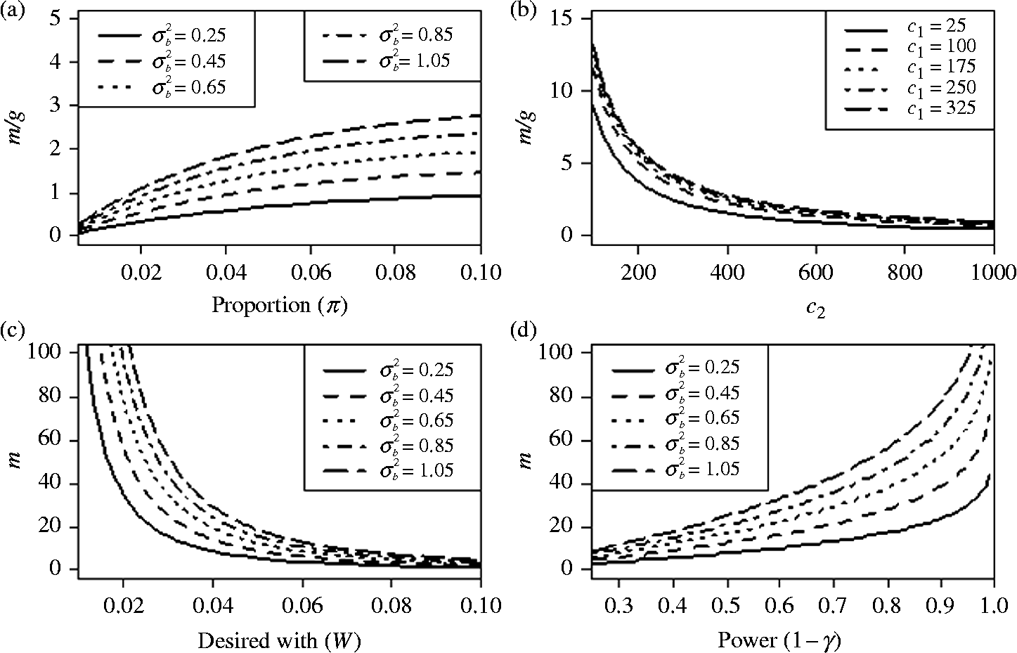
Figure 1 Ratio of the number of clusters and number of pools per cluster. (a) Ratio of the number of clusters and number of pools per cluster m/g as a function of the proportion (
 $$\tilde {>\pi } $$
), for
$$\tilde {>\pi } $$
), for
 $$C = 10,000 $$
,
$$C = 10,000 $$
,
 $$c _{1} = 250, c _{2} = 800, s = 10, S _{ e } = 0.98, S _{ p } = 0.96 $$
and five different values of
$$c _{1} = 250, c _{2} = 800, s = 10, S _{ e } = 0.98, S _{ p } = 0.96 $$
and five different values of
 $$\sigma _{ b }^{2} $$
. (b) Ratio of m/g as a function of
$$\sigma _{ b }^{2} $$
. (b) Ratio of m/g as a function of
 $$c _{2} $$
, for
$$c _{2} $$
, for
 $$C = 10,000 $$
,
$$C = 10,000 $$
,
 $$\sigma _{ b }^{2} = 0.5, \tilde {>\pi } = 0.05 $$
,
$$\sigma _{ b }^{2} = 0.5, \tilde {>\pi } = 0.05 $$
,
 $$s = 10, S _{ e } = 0.98, S _{ p } = 0.96 $$
and several values of
$$s = 10, S _{ e } = 0.98, S _{ p } = 0.96 $$
and several values of
 $$c _{1} $$
. (c) Required number of clusters, m, as a function of the desired confidence interval width
$$c _{1} $$
. (c) Required number of clusters, m, as a function of the desired confidence interval width
 $$\left ( \omega \right ) $$
, for
$$\left ( \omega \right ) $$
, for
 $$c _{1} = 50, c _{2} = 1600, \tilde {>\pi } = 0.05, s = 10, S _{ e } = 0.98, S _{ p } = 0.96 $$
, and five different values of
$$c _{1} = 50, c _{2} = 1600, \tilde {>\pi } = 0.05, s = 10, S _{ e } = 0.98, S _{ p } = 0.96 $$
, and five different values of
 $$\sigma _{ b }^{2} $$
. (d) Required number of clusters, m, as a function of the desired power
$$\sigma _{ b }^{2} $$
. (d) Required number of clusters, m, as a function of the desired power
 $$(1 - \gamma ) $$
, for
$$(1 - \gamma ) $$
, for
 $$c _{1} = 50, c _{2} = 1600, \tilde {>\pi } = 0.04, d = 0.015, s = 10, S _{ e } = 0.98,S_{ p } = 0.96, \alpha = 0.05 $$
and five different values of
$$c _{1} = 50, c _{2} = 1600, \tilde {>\pi } = 0.04, d = 0.015, s = 10, S _{ e } = 0.98,S_{ p } = 0.96, \alpha = 0.05 $$
and five different values of
 $$\sigma _{ b }^{2} $$
.
$$\sigma _{ b }^{2} $$
.
Figure 1b illustrates the behaviour of the ratio (m/g) as a function of the cost of enrolling clusters in the study
 $$c _{2} $$
. As
$$c _{2} $$
. As
 $$c _{2} $$
increases, the ratio (m/g) decreases, which is expected since the cost of including a cluster increases relative to the cost of enrolling pools, which does not change. Figure 1c shows that the number of clusters, m, decreases as the expected width of the CI increases (
$$c _{2} $$
increases, the ratio (m/g) decreases, which is expected since the cost of including a cluster increases relative to the cost of enrolling pools, which does not change. Figure 1c shows that the number of clusters, m, decreases as the expected width of the CI increases (
 $$\omega $$
), which makes sense, since a narrow expected width (
$$\omega $$
), which makes sense, since a narrow expected width (
 $$\omega $$
) of the CI implies that the estimation process is more precise, and vice versa. In Fig. 1d, we can see that the required number of clusters, m, increases when a larger power is required.
$$\omega $$
) of the CI implies that the estimation process is more precise, and vice versa. In Fig. 1d, we can see that the required number of clusters, m, increases when a larger power is required.
Correction factor for unequal cluster sizes
Although equal cluster sizes are optimal for estimating the proportion of interest, they are rarely encountered in practice. Variation in the actual size of the clusters (fields, localities, hospital, schools, etc.), non-response and dropout of individuals (among others) generate unequal cluster sizes in a study (Van Breukelen et al., Reference Van Breukelen, Candel and Berger2007). Cluster size variation increases bias and causes considerable loss of power and precision in the parameter estimates. For this reason, we will calculate the relative efficiency of unequal versus equal cluster sizes for adjusting the optimal sample size under the assumption of equal cluster sizes. The relative efficiency of equal versus unequal cluster sizes for the estimator of the proportion of interest,
 $$RE ( \circ {>\pi } ) $$
, is defined as:
$$RE ( \circ {>\pi } ) $$
, is defined as:
 $$ RE \left ( \circ {>\pi } \right ) = \frac {Var\left ( \circ {>\pi } \vert \varsigma _{equal}\right )}{Var\left ( \circ {>\pi } \vert \varsigma _{unequal}\right )} $$
where
 $$Var\left ( \circ {>\pi } \vert \varsigma _{equal}\right ) $$
denotes the variance of the proportion estimator given a design with equal cluster sizes,
$$Var\left ( \circ {>\pi } \vert \varsigma _{equal}\right ) $$
denotes the variance of the proportion estimator given a design with equal cluster sizes,
 $$Var\left ( \circ {>\pi } \vert \varsigma _{unequal}\right ) $$
denotes a similar value for an unequal cluster size design, but with the same number of clusters m and the same total number of pools
$$Var\left ( \circ {>\pi } \vert \varsigma _{unequal}\right ) $$
denotes a similar value for an unequal cluster size design, but with the same number of clusters m and the same total number of pools
 $$( N = { \sum _{ i = 1}^{ m } }\, g _{ i }) $$
as in the equal cluster size design. Thus
$$( N = { \sum _{ i = 1}^{ m } }\, g _{ i }) $$
as in the equal cluster size design. Thus
 $$RE \left ( \circ {>\pi } \right ) $$
is equal to:
$$RE \left ( \circ {>\pi } \right ) $$
is equal to:
 $$ RE \left ( \circ {>\pi } \right ) = \frac {( \sigma _{ b }^{2\ast } + V ( \delta )/ \bar {>g} )/ m }{{ \sum _{ i = 1}^{ m } }\,[( \sigma _{ b }^{2\ast } + V ( \delta )/ g _{ i }]/ m ^{2}} = \frac { \bar {>g} + \alpha }{ \bar {>g} }\frac {1}{ m }{ \sum _{ i = 1}^{ m } }\,\left [\frac { g _{ i }}{ g _{ i } + \alpha }\right ] $$
where
 $$\sigma _{ b }^{2\ast } = \left \{ \tilde {>\pi } \left (1 - \tilde {>\pi } \right )\right \}^{2} \sigma _{ b }^{2} $$
and
$$\sigma _{ b }^{2\ast } = \left \{ \tilde {>\pi } \left (1 - \tilde {>\pi } \right )\right \}^{2} \sigma _{ b }^{2} $$
and
 $$\alpha = V ( \delta )/ \sigma _{ b }^{2\ast } $$
. Note that equation (21) is equal to that derived for the RE of equal versus unequal cluster sizes in cluster randomized and multicentre trials given by Van Breukelen et al. (Reference Van Breukelen, Candel and Berger2007) to recover the loss of power when estimating treatment effects using a linear model. Here we use RE to repair the loss of power or precision when estimating the proportion using a random logistic model for group testing. Since our RE was expressed as that derived by Van Breukelen et al. (Reference Van Breukelen, Candel and Berger2007), we use their approach to obtain a Taylor series approximation of equation (21), expressing the RE as a function of the intraclass correlation
$$\alpha = V ( \delta )/ \sigma _{ b }^{2\ast } $$
. Note that equation (21) is equal to that derived for the RE of equal versus unequal cluster sizes in cluster randomized and multicentre trials given by Van Breukelen et al. (Reference Van Breukelen, Candel and Berger2007) to recover the loss of power when estimating treatment effects using a linear model. Here we use RE to repair the loss of power or precision when estimating the proportion using a random logistic model for group testing. Since our RE was expressed as that derived by Van Breukelen et al. (Reference Van Breukelen, Candel and Berger2007), we use their approach to obtain a Taylor series approximation of equation (21), expressing the RE as a function of the intraclass correlation
 $$\rho $$
, and the mean and standard deviation of cluster size. It is important to point out that equation (21) is expressed in terms of pools instead of individuals, as in the formula of Van Breukelen et al. (Reference Van Breukelen, Candel and Berger2007). Therefore, we assumed that the cluster sizes
$$\rho $$
, and the mean and standard deviation of cluster size. It is important to point out that equation (21) is expressed in terms of pools instead of individuals, as in the formula of Van Breukelen et al. (Reference Van Breukelen, Candel and Berger2007). Therefore, we assumed that the cluster sizes
 $$g _{ i }( i = 1,2,\ldots , m ) $$
are realizations of a random variable U having mean
$$g _{ i }( i = 1,2,\ldots , m ) $$
are realizations of a random variable U having mean
 $$\mu _{ g } $$
and standard deviation
$$\mu _{ g } $$
and standard deviation
 $$\sigma _{ g } $$
. According to Van Breukelen et al. (Reference Van Breukelen, Candel and Berger2007), equation (21) can be considered a moment estimator of
$$\sigma _{ g } $$
. According to Van Breukelen et al. (Reference Van Breukelen, Candel and Berger2007), equation (21) can be considered a moment estimator of
 $$ RE \left ( \circ {>\pi } \right ) = \frac { \bar {>g} + \alpha }{ \bar {>g} } E \left (\frac { U }{ U + \alpha }\right ). $$
If we define
 $$\lambda = ( \mu _{ g } $$
/(
$$\lambda = ( \mu _{ g } $$
/(
 $$\mu _{ g } $$
+
$$\mu _{ g } $$
+
 $$\, \alpha )) $$
, and the coefficient of variation of the random variable U by
$$\, \alpha )) $$
, and the coefficient of variation of the random variable U by
 $$CV = \sigma _{ g }/ \mu _{ g } $$
, then by using derivations similar to those reported by Van Breukelen et al. (Reference Van Breukelen, Candel and Berger2007, pp. 2601–2602; see Appendix D), we obtain the following second-order Taylor approximation of the expectation part of equation (22)
$$CV = \sigma _{ g }/ \mu _{ g } $$
, then by using derivations similar to those reported by Van Breukelen et al. (Reference Van Breukelen, Candel and Berger2007, pp. 2601–2602; see Appendix D), we obtain the following second-order Taylor approximation of the expectation part of equation (22)
 $$E (\frac { U }{ U + \alpha })\approx \lambda \{1 - CV ^{2} \lambda \left (1 - \lambda \right )\} $$
. The second-order Taylor approximation of equation (21) is:
$$E (\frac { U }{ U + \alpha })\approx \lambda \{1 - CV ^{2} \lambda \left (1 - \lambda \right )\} $$
. The second-order Taylor approximation of equation (21) is:
 $$ RE \left ( \circ {>\pi } \right )_{ t }\approx \left \{1 - CV ^{2} \lambda \left (1 - \lambda \right )\right \}. $$
It is evident that
 $$RE \left ( \circ {>\pi } \right )_{ t } $$
does not depend on the number of clusters m, but rather on the distribution of cluster sizes (mean and variance) and intraclass correlations. When
$$RE \left ( \circ {>\pi } \right )_{ t } $$
does not depend on the number of clusters m, but rather on the distribution of cluster sizes (mean and variance) and intraclass correlations. When
 $$\sigma _{ b }^{2\ast }\rightarrow 0 $$
(and thus
$$\sigma _{ b }^{2\ast }\rightarrow 0 $$
(and thus
 $$\rho \rightarrow 0) $$
or
$$\rho \rightarrow 0) $$
or
 $$\sigma _{ b }^{2\ast }\rightarrow \infty $$
(and thus
$$\sigma _{ b }^{2\ast }\rightarrow \infty $$
(and thus
 $$\rho \rightarrow 1) $$
, we have
$$\rho \rightarrow 1) $$
, we have
 $$RE \rightarrow 1 $$
. For
$$RE \rightarrow 1 $$
. For
 $$0\lt \sigma _{ b }^{2\ast }\lt \infty $$
(and thus
$$0\lt \sigma _{ b }^{2\ast }\lt \infty $$
(and thus
 $$0\lt \rho \lt 1) $$
, we can see that
$$0\lt \rho \lt 1) $$
, we can see that
 $$RE \lt 1 $$
, implying that equal cluster sizes are optimal. For practical purposes, we will denote
$$RE \lt 1 $$
, implying that equal cluster sizes are optimal. For practical purposes, we will denote
 $$RE \left ( \circ {>\pi } \right )_{ t } = RE _{ t } $$
. To correct for the loss of efficiency due to the assumption of equal cluster sizes, one simply divides the number of clusters (m) given in equation (15) or (16) by the expected RE resulting from equation (23). Also, it is evident that the number of clusters will increase the budget to
$$RE \left ( \circ {>\pi } \right )_{ t } = RE _{ t } $$
. To correct for the loss of efficiency due to the assumption of equal cluster sizes, one simply divides the number of clusters (m) given in equation (15) or (16) by the expected RE resulting from equation (23). Also, it is evident that the number of clusters will increase the budget to
 $$C^{\ast } = C\left (\frac {1}{ RE _{ t }}\right ) $$
, whereas the optimal number of pools per cluster (g) does not change.
$$C^{\ast } = C\left (\frac {1}{ RE _{ t }}\right ) $$
, whereas the optimal number of pools per cluster (g) does not change.
Comparison of the relative efficiency and its Taylor approximation
To compare the RE of equation (21), its Taylor approximation (equation 23) was performed for four cluster size distributions: uniform, unimodal, bimodal and positively skewed. Three different cluster sizes,
 $$g _{ a }, g _{ b }, g _{ c } $$
, with frequencies
$$g _{ a }, g _{ b }, g _{ c } $$
, with frequencies
 $$f _{ a }, f _{ b }, f _{ c } $$
, were evaluated (see Table 1). For each of the four distributions, both REs [asymptotic (equation 21) and Taylor approximation (equation 23)] were computed and plotted as a function of the intraclass correlation (the values used were from 0.0 to 0.3).
$$f _{ a }, f _{ b }, f _{ c } $$
, were evaluated (see Table 1). For each of the four distributions, both REs [asymptotic (equation 21) and Taylor approximation (equation 23)] were computed and plotted as a function of the intraclass correlation (the values used were from 0.0 to 0.3).
Table 1 Cluster size distribution used for calculating relative efficiency

 $$f _{ a } $$
number of clusters of size
$$f _{ a } $$
number of clusters of size
 $$g _{ a } $$
(small),
$$g _{ a } $$
(small),
 $$f _{ b } $$
number of clusters of size
$$f _{ b } $$
number of clusters of size
 $$g _{ b } $$
(medium),
$$g _{ b } $$
(medium),
 $$f _{ c } $$
number of clusters of size
$$f _{ c } $$
number of clusters of size
 $$g _{ c } $$
(large); CV = coefficient of variation. Two numbers of clusters were studied: m= 18 with average pools per cluster
$$g _{ c } $$
(large); CV = coefficient of variation. Two numbers of clusters were studied: m= 18 with average pools per cluster
 $$\bar {>g} = 22 $$
, and m= 48 with average pools per cluster
$$\bar {>g} = 22 $$
, and m= 48 with average pools per cluster
 $$\bar {>g} = 20 $$
. In both cases, the pool size was s= 10.
$$\bar {>g} = 20 $$
. In both cases, the pool size was s= 10.
Figure 2 shows that for the four distributions (uniform, unimodal, bimodal and positively skewed), the RE drops from 1 at
 $$\rho = 0 $$
to minimum at
$$\rho = 0 $$
to minimum at
 $$\rho $$
somewhere between
$$\rho $$
somewhere between
 $$\rho = 0.05 $$
and 0.1, and then increases, returning to 1 for
$$\rho = 0.05 $$
and 0.1, and then increases, returning to 1 for
 $$\rho = 1 $$
. Lower RE values are observed when there is more cluster size variation (as in the case of bimodal distribution with larger values of CV>0.70). For this reason, by comparing the four distributions, we can see in Fig. 2 that the positively skewed distribution gives the highest RE, followed by the unimodal, uniform and bimodal distributions. These results are in line with results reported by Van Breukelen et al. (Reference Van Breukelen, Candel and Berger2007, Reference Van Breukelen, Candel and Berger2008) and Candel and Van Breukelen (Reference Candel and Van Breukelen2010) for studies of cluster randomized trials for normal data and binary results in a non-group testing context.
$$\rho = 1 $$
. Lower RE values are observed when there is more cluster size variation (as in the case of bimodal distribution with larger values of CV>0.70). For this reason, by comparing the four distributions, we can see in Fig. 2 that the positively skewed distribution gives the highest RE, followed by the unimodal, uniform and bimodal distributions. These results are in line with results reported by Van Breukelen et al. (Reference Van Breukelen, Candel and Berger2007, Reference Van Breukelen, Candel and Berger2008) and Candel and Van Breukelen (Reference Candel and Van Breukelen2010) for studies of cluster randomized trials for normal data and binary results in a non-group testing context.
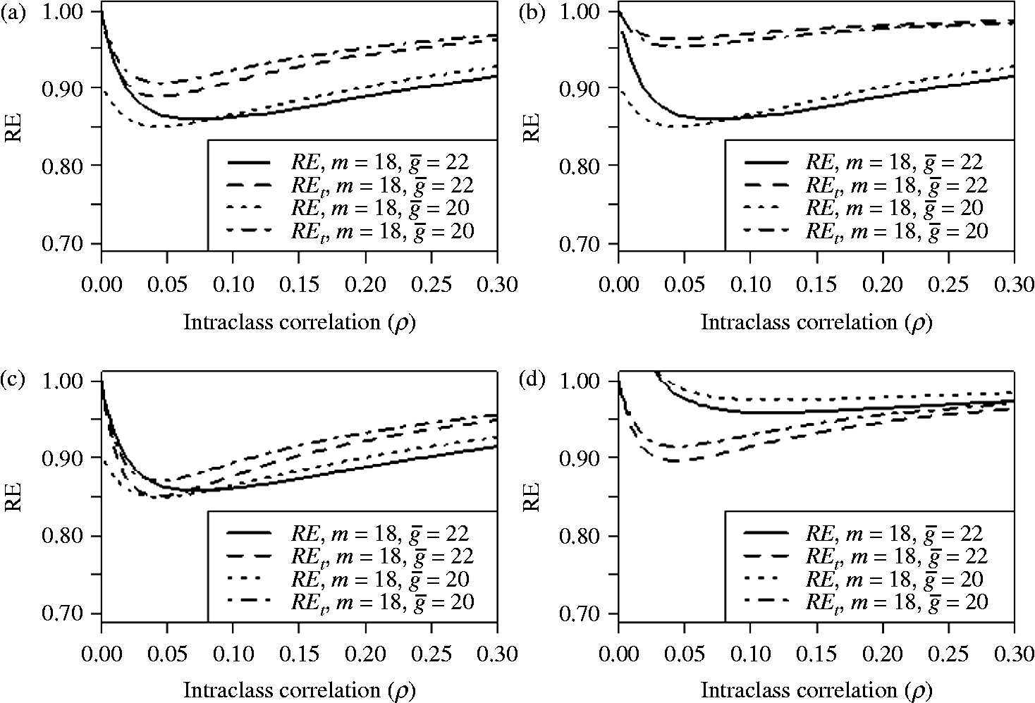
Figure 2 Relative efficiency of unequal versus equal cluster sizes as a function of the intraclass correlation
 $$( \rho ) $$
for four distributions of cluster size: (a) uniform, (b) unimodal, (c) bimodal and (d) positively skewed distribution.
$$( \rho ) $$
for four distributions of cluster size: (a) uniform, (b) unimodal, (c) bimodal and (d) positively skewed distribution.
Figure 2 also shows that the Taylor approximation (equation 23, denoted as
 $$RE _{ t } $$
) of the RE given in equation (21) is acceptable in most cases. However, it is clearly affected by the distribution of the cluster sizes, the number of clusters, the number of pools per cluster and the value of the intraclass correlation.
$$RE _{ t } $$
) of the RE given in equation (21) is acceptable in most cases. However, it is clearly affected by the distribution of the cluster sizes, the number of clusters, the number of pools per cluster and the value of the intraclass correlation.
Estimating the proportion of transgenic plants – An example
Next we illustrate how to achieve the optimal allocation of fields and pools for minimizing the variance (using equation 15), and for estimating the required budget for a desired CI width and the budget required to obtain a certain power (using equation 16). Carreón-Herrera (Reference Carreón-Herrera2011) collected corn grain in 14 localities of the Sierra Nororiental and 22 localities in the Mixteca Baja, in the State of Puebla, Mexico. She collected a total of 58 kg of grain. Forty-seven samples were obtained from farmers and 11 from DICONSA stores. Of the 58 samples, 36 were white grain, 10 yellow, 8 blue and 4 red. The researchers used the polymerase chain reaction (PCR) to detect the promoter of cauliflower mosaic virus (CaMV-35S), which indicates the presence of transgenic corn. They reported the percentage of the CaMV-35S promoter in each sample. The standard 0.01% was used as the lower limit of reference for the detection of CaMV-35S. The percentages of the CaMV-35S promoter reported varied between 0.01% and 0.25%. However, in a study conducted in the neighbouring state of Oaxaca, Landavazo Gamboa et al. (Reference Landavazo Gamboa, Calvillo Alba, Espinosa Huerta, González Morelos, Aragón Cuevas, Torres Pacheco and Mora Avilés2006) reported a lower value (0.000012% median for the five fields studied) for the percentage of the CaMV-35S promoter. Assuming that we wish to conduct another study in this region of Puebla, we can assume that the expected proportion of transgenes is equal to
 $$\tilde {>\pi } = \frac {0.0025 - 0.00000012}{2} = 0.0013 $$
, while the variance between clusters
$$\tilde {>\pi } = \frac {0.0025 - 0.00000012}{2} = 0.0013 $$
, while the variance between clusters
 $$\sigma ^{2} = (\frac {range}{6})^{2} $$
. For binomial data, the range relevant to six-sigma approximation is the difference between the maximum and minimum plausible logit (Stroup, Reference Stroup2012). Since we know the lowest (
$$\sigma ^{2} = (\frac {range}{6})^{2} $$
. For binomial data, the range relevant to six-sigma approximation is the difference between the maximum and minimum plausible logit (Stroup, Reference Stroup2012). Since we know the lowest (
 $$\tilde {>\pi } _{ L } = 0.00000012) $$
and highest (
$$\tilde {>\pi } _{ L } = 0.00000012) $$
and highest (
 $$\tilde {>\pi } _{ H } = 0.0025) $$
plausible probabilities, we can calculate the logit
$$\tilde {>\pi } _{ H } = 0.0025) $$
plausible probabilities, we can calculate the logit
 $$l _{ L } = \,log\,\left [\frac { \tilde {>\pi } _{ L }}{1 - \tilde {>\pi } _{ L }}\right ] = \,log\,\left [\frac {0.00000012}{1 - 0.00000012}\right ] = - 6.9208 $$
and
$$l _{ L } = \,log\,\left [\frac { \tilde {>\pi } _{ L }}{1 - \tilde {>\pi } _{ L }}\right ] = \,log\,\left [\frac {0.00000012}{1 - 0.00000012}\right ] = - 6.9208 $$
and
 $$l _{ H } = \,log\,\left [\frac { \tilde {>\pi } _{ H }}{1 - \tilde {>\pi } _{ H }}\right ] = \,log\,\left [\frac {0.0025}{1 - 0.0025}\right ] = - 2.60\,097 $$
; then the range is equal to range = − 2.6009+6.9208 = 4.3196. Therefore,
$$l _{ H } = \,log\,\left [\frac { \tilde {>\pi } _{ H }}{1 - \tilde {>\pi } _{ H }}\right ] = \,log\,\left [\frac {0.0025}{1 - 0.0025}\right ] = - 2.60\,097 $$
; then the range is equal to range = − 2.6009+6.9208 = 4.3196. Therefore,
 $$\sigma _{ b }^{2}\cong (4.3196/6)^{2} = 0.5184 $$
. Based on a literature review, we decided to use a pool size of 10 plants per pool,
$$\sigma _{ b }^{2}\cong (4.3196/6)^{2} = 0.5184 $$
. Based on a literature review, we decided to use a pool size of 10 plants per pool,
 $$S _{ e } = 0.999 $$
,
$$S _{ e } = 0.999 $$
,
 $$S _{ p } = 0.997 $$
,
$$S _{ p } = 0.997 $$
,
 $$C = 20,000 $$
total budget for the study,
$$C = 20,000 $$
total budget for the study,
 $$c _{2} = 850 $$
cost of enrolling fields in the study, and
$$c _{2} = 850 $$
cost of enrolling fields in the study, and
 $$c _{1} = 70 $$
cost of enrolling pools composed of
$$c _{1} = 70 $$
cost of enrolling pools composed of
 $$s = 10 $$
plants in the study. Next we obtained the required sample sizes for minimizing the variance, for achieving a certain width of the CI and for obtaining a certain power.
$$s = 10 $$
plants in the study. Next we obtained the required sample sizes for minimizing the variance, for achieving a certain width of the CI and for obtaining a certain power.
Minimizing the variance
Computing
 $$\tilde {>\pi } ^{ p } = 0.999 + (1 - 0.999 - 0.997)(1 - 0.0013)^{10} $$
 $$= 0.01\,587 $$
and
$$= 0.01\,587 $$
and
 $$V ( \delta ) = \frac {\left (\, S _{ e } - \tilde {>\pi } ^{ p }\right )^{\frac {2}{ s } - 2} \tilde {>\pi } ^{ p }(1 - \tilde {>\pi } ^{ p })}{ s ^{2}( S _{ e } + S _{ p } - 1)^{2/ s }} $$
 $$= \frac {\left (0.999 - 0.01\,587\right )^{\frac {2}{10} - 2}(0.01\,587)(1 - 0.01\,587)}{10^{2}(0.999 + 0.997 - 1)^{2/10}} = 0.000161 $$
results in
$$= \frac {\left (0.999 - 0.01\,587\right )^{\frac {2}{10} - 2}(0.01\,587)(1 - 0.01\,587)}{10^{2}(0.999 + 0.997 - 1)^{2/10}} = 0.000161 $$
results in
 $$\begin{eqnarray} g = \sqrt {\frac {850}{70}}\frac {\sqrt {0.000161}}{0.0013(1 - 0.0013)\sqrt {0.5184}} = 47.32\,856\approx 47 \end{eqnarray}$$
 $$m = \frac { C }{ c _{2} + gc _{1}} = \frac {20\,000}{850 + (51)(70)} = 4.8042\approx 5. $$
This means that we need to select five fields at random from the population of fields, with 47 pools in each field. Thus the total number of plants to select from each field is
 $$g \times s = 47\times 10 = 470 $$
plants, which will be allocated at random to form the 47 pools.
$$g \times s = 47\times 10 = 470 $$
plants, which will be allocated at random to form the 47 pools.
Now, if the cluster sizes are unequal, how do we compensate for the loss of efficiency due to varying cluster sizes? Assuming that the mean and standard deviation of cluster sizes are
 $$\mu _{ g } = 177 $$
and
$$\mu _{ g } = 177 $$
and
 $$\sigma _{ g } = 81.5 $$
, respectively, then
$$\sigma _{ g } = 81.5 $$
, respectively, then
 $$CV = \frac {81.5}{177} = 0.4605 $$
,
$$CV = \frac {81.5}{177} = 0.4605 $$
,
 $$\alpha = \frac { V ( \delta )}{ \sigma _{ b }^{2}\ast } = \frac {0.000161}{\left \{0.0013\left (1 - 0.0013\right )\right \}^{2}0.5184} = 5 $$
, so
$$\alpha = \frac { V ( \delta )}{ \sigma _{ b }^{2}\ast } = \frac {0.000161}{\left \{0.0013\left (1 - 0.0013\right )\right \}^{2}0.5184} = 5 $$
, so
 $$\lambda = (177/(177 + 5) = 0.9602 $$
. Therefore,
$$\lambda = (177/(177 + 5) = 0.9602 $$
. Therefore,
 $$RE _{ t } = $$
 $$\{1 - (0.4605^{2})(0.9725)\left (1 - 0.9725\right )\} = 0.9943 $$
and, for practical purposes, adjustment for unequal cluster sizes is not needed. However, to illustrate the method, full efficiency can be restored by taking
$$\{1 - (0.4605^{2})(0.9725)\left (1 - 0.9725\right )\} = 0.9943 $$
and, for practical purposes, adjustment for unequal cluster sizes is not needed. However, to illustrate the method, full efficiency can be restored by taking
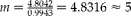 $$m = \frac {4.8042}{0.9943} = 4.8316\approx 5 $$
clusters with g= 47 pools, and the new total budget will increase to
$$m = \frac {4.8042}{0.9943} = 4.8316\approx 5 $$
clusters with g= 47 pools, and the new total budget will increase to
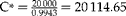 $$C\ast = \frac {20\,000}{0.9943} = 20\,114.65 $$
.
$$C\ast = \frac {20\,000}{0.9943} = 20\,114.65 $$
.
Specified CI width
Now suppose that the researcher requires a 95% confidence interval estimate, with a desired width for the proportion of transgenic plants that is equal to
 $$W = ( \tilde {>\pi } _{ U } - \tilde {>\pi } _{ L })\leq \omega = 0.0025 $$
. Therefore,
$$W = ( \tilde {>\pi } _{ U } - \tilde {>\pi } _{ L })\leq \omega = 0.0025 $$
. Therefore,
 $$Z _{1 - 0.05/2} = 1.96 $$
and
$$Z _{1 - 0.05/2} = 1.96 $$
and
 $$V _{0} = \omega ^{2} $$
/4
$$V _{0} = \omega ^{2} $$
/4
 $$Z _{1 - \alpha /2}^{2} = \frac {0.0025^{2}}{4\ast 1.96^{2}} = 0.000000401 $$
. Using the same values of
$$Z _{1 - \alpha /2}^{2} = \frac {0.0025^{2}}{4\ast 1.96^{2}} = 0.000000401 $$
. Using the same values of
 $$s , S _{ e }, S _{ p }, $$
 $$\sigma _{ b }^{2}, \tilde {>\pi } , c _{2} $$
and c
1 as given for minimizing the variance, equation (16) gives
$$\sigma _{ b }^{2}, \tilde {>\pi } , c _{2} $$
and c
1 as given for minimizing the variance, equation (16) gives
 $$g = \sqrt {\frac {850}{70}}\frac {\sqrt {0.000161}}{0.0013(1 - 0.0013)\sqrt {0.5184}} = 47 $$
, while the number of clusters is equal to:
$$g = \sqrt {\frac {850}{70}}\frac {\sqrt {0.000161}}{0.0013(1 - 0.0013)\sqrt {0.5184}} = 47 $$
, while the number of clusters is equal to:
 $$\begin{eqnarray} m = \frac {\left [\left \{0.0013\left (1 - 0.0013\right )\right \}^{2}\left (0.5184\right ) + \frac {0.000161}{47}\right ]}{0.000000401} = 10.5802\approx 11. \end{eqnarray}$$
Since the value of g does not change, we need 470 plants per field, but now we need 11 fields to reach the required width of a 95% CI. However, this sample size is valid only for equal cluster sizes. If needed, adjustment for unequal cluster sizes is carried out by
 $$m \ast = \frac { m }{ RE _{ t }} $$
.
$$m \ast = \frac { m }{ RE _{ t }} $$
.
Therefore the budget has to be equal to
 $$C = \left (47\right )\left (11\right )\left (70\right ) + 11\left (850\right ) = $$
45,540. This implies that the required total budget for obtaining a 95% CI for estimating the proportion
$$C = \left (47\right )\left (11\right )\left (70\right ) + 11\left (850\right ) = $$
45,540. This implies that the required total budget for obtaining a 95% CI for estimating the proportion
 $$\left ( \tilde {>\pi } \right ) $$
with a desired width of 0.0025 is 2.264 times larger than the previous budget (20,114.65).
$$\left ( \tilde {>\pi } \right ) $$
with a desired width of 0.0025 is 2.264 times larger than the previous budget (20,114.65).
Now we determine the required number of clusters when there is no budget constraint, and assuming g= 10 (pools per cluster). Using equation (17) and assuming the same values of
 $$\omega , s , \alpha , S _{ e }, S _{ p }, \sigma _{ b }^{2}, \tilde {>\pi } $$
as were given for minimizing the variance, we have
$$\omega , s , \alpha , S _{ e }, S _{ p }, \sigma _{ b }^{2}, \tilde {>\pi } $$
as were given for minimizing the variance, we have
 $$\begin{eqnarray} m = \frac {4(1.96)^{2}}{0.0025^{2}}\left [\left \{0.0013\left (1 - 0.0013\right )\right \}^{2}(0.5184) + \frac {0.000161}{10}\right ] = 41.7783\approx 42. \end{eqnarray}$$
This implies that we need a sample of 42 clusters, each containing 10 pools, assuming equal cluster size. Using unequal cluster sizes and assuming the same mean and standard deviation of cluster sizes, we need
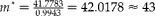 $$m ^{\ast } = \frac {41.7783}{0.9943} = 42.0178\approx 43 $$
clusters. Of course, in this case, the total budget will be higher than the previously specified budget.
$$m ^{\ast } = \frac {41.7783}{0.9943} = 42.0178\approx 43 $$
clusters. Of course, in this case, the total budget will be higher than the previously specified budget.
Specified power
Now suppose that we need to know the budget and sample size required for testing
 $$H _{0}: \tilde {>\pi } _{0} = 0.0013 $$
versus
$$H _{0}: \tilde {>\pi } _{0} = 0.0013 $$
versus
 $$H _{1}: \tilde {>\pi } _{0}> 0.0013 $$
at an
$$H _{1}: \tilde {>\pi } _{0}> 0.0013 $$
at an
 $$\alpha = 0.05 $$
significance level with a power
$$\alpha = 0.05 $$
significance level with a power
 $$(1 - \gamma ) = 0.9 $$
(90%) for detecting
$$(1 - \gamma ) = 0.9 $$
(90%) for detecting
 $$\delta \geq 0.002 $$
and using the same parameter values (
$$\delta \geq 0.002 $$
and using the same parameter values (
 $$s , S _{ e }, S _{ p }, \sigma _{ b }^{2}, c _{2} $$
and c
1) as before. Then,
$$s , S _{ e }, S _{ p }, \sigma _{ b }^{2}, c _{2} $$
and c
1) as before. Then,
 $$V _{0} = V _{2} = \frac {0.002^{2}}{\left (1.645 + 1.282\right )^{2}} = 0.0000004671 $$
. Since
$$V _{0} = V _{2} = \frac {0.002^{2}}{\left (1.645 + 1.282\right )^{2}} = 0.0000004671 $$
. Since
 $$V ( \delta _{0}) = V \left ( \delta \right ) = 0.000161 $$
,
$$V ( \delta _{0}) = V \left ( \delta \right ) = 0.000161 $$
,
 $$\tilde {>\pi } = \tilde {>\pi } _{0} $$
, then
$$\tilde {>\pi } = \tilde {>\pi } _{0} $$
, then
 $$g = \sqrt {\frac {850}{70}}\frac {\sqrt {0.000161}}{0.0013(1 - 0.0013)\sqrt {0.5184}}\approx 47 $$
, and the required number of clusters is equal to:
$$g = \sqrt {\frac {850}{70}}\frac {\sqrt {0.000161}}{0.0013(1 - 0.0013)\sqrt {0.5184}}\approx 47 $$
, and the required number of clusters is equal to:
 $$\begin{eqnarray} m = \frac {\left [\left \{0.0013\left (1 - 0.0013\right )\right \}^{2}\left (0.5184\right ) + \frac {0.000161}{47}\right ]}{0.000105} = 9.2136\approx 10. \end{eqnarray}$$
Here, too, we need 470 plants per field, but now we need 10 fields to reach the required power of 90%. To compensate for the unequal cluster sizes and assuming the same mean and standard deviation of the cluster sizes (
 $$\mu _{ g } = 177 $$
and
$$\mu _{ g } = 177 $$
and
 $$\sigma _{ g } = 81.5 $$
), we multiply
$$\sigma _{ g } = 81.5 $$
), we multiply
 $$m = 9.2136 $$
by the correction factor (1/0.9943), which gives us
$$m = 9.2136 $$
by the correction factor (1/0.9943), which gives us
 $$m ^{\ast } = \frac {9.2136}{0.9943} = 9.2664\approx 10 $$
clusters. Here the number of clusters remains the same due to rounding, but this is not always the case.
$$m ^{\ast } = \frac {9.2136}{0.9943} = 9.2664\approx 10 $$
clusters. Here the number of clusters remains the same due to rounding, but this is not always the case.
Here, also, the required budget is C = (10)(47)(70)+10(850) = 41,400 which implies that the required total budget is 2.058 times larger than the budget for minimizing the variance of the proportion (20,114.65). However, this case guarantees a power of 90% for
 $$\delta \geq 0.002 $$
.
$$\delta \geq 0.002 $$
.
Now consider the problem without a budget constraint with 10 pools per cluster (g); solving for the required number of clusters (m) using the same values of
 $$s , S _{ e }, S _{ p }, \sigma _{ b }^{2}, \alpha ,(1 - \gamma ) $$
,
$$s , S _{ e }, S _{ p }, \sigma _{ b }^{2}, \alpha ,(1 - \gamma ) $$
,
 $$\delta = \tilde {>\pi } _{1} - \tilde {>\pi } _{0} $$
as above, gives
$$\delta = \tilde {>\pi } _{1} - \tilde {>\pi } _{0} $$
as above, gives
 $$\begin{eqnarray} m = \frac {\left (1.645 + 1.282\right )^{2}}{0.002^{2}}\left [\left \{0.0013\left (1 - 0.0013\right )\right \}^{2}(0.5184) + \frac {0.000161}{10}\right ] = 44.6386. \end{eqnarray}$$
This means that to perform the study, we need 45 clusters with 10 pools per cluster if the cluster sizes are equal, and
 $$m ^{\ast } = \frac {44.6386}{0.9943} = 44.8945\approx 45 $$
clusters using unequal cluster sizes.
$$m ^{\ast } = \frac {44.6386}{0.9943} = 44.8945\approx 45 $$
clusters using unequal cluster sizes.
Tables for determining sample size
This section contains tables that help to calculate the optimal sample size. Table 2 gives the optimal allocation of clusters and pools when the goal is to estimate the proportion (
 $$\tilde {>\pi } $$
) with minimum variance using group testing with pool size (s= 10). The cost function is C = mgc
1+mc
2 with C = 10,000, with six values of
$$\tilde {>\pi } $$
) with minimum variance using group testing with pool size (s= 10). The cost function is C = mgc
1+mc
2 with C = 10,000, with six values of
 $$\sigma _{ b }^{2} = 0.15,0.25,0.45,0.65,0.85,1.05 $$
; three values of
$$\sigma _{ b }^{2} = 0.15,0.25,0.45,0.65,0.85,1.05 $$
; three values of
 $$c _{1} = 50,100,200 $$
and
$$c _{1} = 50,100,200 $$
and
 $$c _{2} = 800 $$
. To illustrate how to use Table 2, assume that the proportion of interest is
$$c _{2} = 800 $$
. To illustrate how to use Table 2, assume that the proportion of interest is
 $$\tilde {>\pi } = 0.035 $$
, and that the variance between clusters is
$$\tilde {>\pi } = 0.035 $$
, and that the variance between clusters is
 $$\sigma _{ b }^{2} = 0.25 $$
. Assume the researcher estimates the cost of enrolling clusters in the study as
$$\sigma _{ b }^{2} = 0.25 $$
. Assume the researcher estimates the cost of enrolling clusters in the study as
 $$c _{2} = 800 $$
, that the cost of enrolling pools of size s = 10 is
$$c _{2} = 800 $$
, that the cost of enrolling pools of size s = 10 is
 $$c _{1} = 100 $$
and the total budget for conducting the study is C = 10,000. Since in this case
$$c _{1} = 100 $$
and the total budget for conducting the study is C = 10,000. Since in this case
 $$c _{1} = 100 $$
, we will refer to the second subsection of Table 2. We find the value of
$$c _{1} = 100 $$
, we will refer to the second subsection of Table 2. We find the value of
 $$\tilde {>\pi } = 0.035 $$
in the first column and the value of
$$\tilde {>\pi } = 0.035 $$
in the first column and the value of
 $$\sigma _{ b }^{2} = 0.25 $$
in columns four and five. The values in the intersection between the value of
$$\sigma _{ b }^{2} = 0.25 $$
in columns four and five. The values in the intersection between the value of
 $$\tilde {>\pi } = 0.035 $$
(first column) and the value of
$$\tilde {>\pi } = 0.035 $$
(first column) and the value of
 $$\sigma _{ b }^{2} = 0.25 $$
(columns 4 and 5) are the optimal number of pools per cluster (g= 11) and the number of clusters (m= 6) required.
$$\sigma _{ b }^{2} = 0.25 $$
(columns 4 and 5) are the optimal number of pools per cluster (g= 11) and the number of clusters (m= 6) required.
Table 2 Optimal sample sizes (g and m) for group testing for two stages given a pool size that minimizes the variance of the proportion
 $$( \circ {>\pi } ) $$

With pool size (s= 10), cost function
 $$C = mgc _{1} + mc _{2} $$
with C = 10,000 and
$$C = mgc _{1} + mc _{2} $$
with C = 10,000 and
 $$c _{2} = 800 $$
. For ten values of
$$c _{2} = 800 $$
. For ten values of
 $$\tilde {>\pi } $$
, three values of
$$\tilde {>\pi } $$
, three values of
 $$c _{1} $$
and six values of
$$c _{1} $$
and six values of
 $$\sigma _{ b }^{2} $$
.
$$\sigma _{ b }^{2} $$
.
Table 3 gives the optimal allocations of clusters (m) and pools per cluster (g) to estimate
 $$\tilde {>\pi } $$
with a certain width of the confidence interval under the cost function
$$\tilde {>\pi } $$
with a certain width of the confidence interval under the cost function
 $$C = mgc _{1} + mc _{2} $$
, when
$$C = mgc _{1} + mc _{2} $$
, when
 $$c _{1} = 50 $$
and
$$c _{1} = 50 $$
and
 $$c _{2} = 800 $$
and significance level
$$c _{2} = 800 $$
and significance level
 $$\alpha = 0.05 $$
. Three values of
$$\alpha = 0.05 $$
. Three values of
 $$\sigma _{ b }^{2} = 0.15,0.25,0.5 $$
form the three subsections of Table 3. To illustrate, assume that
$$\sigma _{ b }^{2} = 0.15,0.25,0.5 $$
form the three subsections of Table 3. To illustrate, assume that
 $$\tilde {>\pi } = 0.035 $$
,
$$\tilde {>\pi } = 0.035 $$
,
 $$\sigma _{ b }^{2} = 0.25 $$
,
$$\sigma _{ b }^{2} = 0.25 $$
,
 $$c _{1} = 50 $$
,
$$c _{1} = 50 $$
,
 $$c _{2} = 800 $$
, and the desired width of the confidence interval is equal to
$$c _{2} = 800 $$
, and the desired width of the confidence interval is equal to
 $$\omega = 0.015 $$
. The optimal m and g are obtained where the value of
$$\omega = 0.015 $$
. The optimal m and g are obtained where the value of
 $$\tilde {>\pi } = 0.035 $$
(first column) intersects with the value of
$$\tilde {>\pi } = 0.035 $$
(first column) intersects with the value of
 $$\omega = 0.015 $$
(columns 6 and 7) in the second subsection corresponding to
$$\omega = 0.015 $$
(columns 6 and 7) in the second subsection corresponding to
 $$\sigma _{ b }^{2} = 0.25 $$
. Therefore the optimal numbers of pools per cluster (g) and of clusters (m) are 16 and 4, respectively.
$$\sigma _{ b }^{2} = 0.25 $$
. Therefore the optimal numbers of pools per cluster (g) and of clusters (m) are 16 and 4, respectively.
Table 3 Optimal sample sizes (g and m) for confidence interval estimation using group testing in two stages given a pool size

With pool size (s= 10), cost function
 $$C = mgc _{1} + mc _{2} $$
subject to
$$C = mgc _{1} + mc _{2} $$
subject to
 $$V \left ( \circ {>\pi } \right ) = \omega ^{2} $$
/4
$$V \left ( \circ {>\pi } \right ) = \omega ^{2} $$
/4
 $$Z _{1 - \alpha /2}^{2} $$
with
$$Z _{1 - \alpha /2}^{2} $$
with
 $$c _{1} = 50 $$
,
$$c _{1} = 50 $$
,
 $$c _{2} = 800 $$
and significance level
$$c _{2} = 800 $$
and significance level
 $$\alpha = 0.05 $$
. For ten values of
$$\alpha = 0.05 $$
. For ten values of
 $$\tilde {>\pi } $$
, six values of the expected width of the CI (ω), and three values of
$$\tilde {>\pi } $$
, six values of the expected width of the CI (ω), and three values of
 $$\sigma _{ b }^{2} $$
.
$$\sigma _{ b }^{2} $$
.
Table 4 should be used when testing a hypothesis, that is, when we want to test
 $$H _{0}: \tilde {>\pi } = \tilde {>\pi } _{0} $$
relative to
$$H _{0}: \tilde {>\pi } = \tilde {>\pi } _{0} $$
relative to
 $$H _{1}: \tilde {>\pi } > \tilde {>\pi } _{0} $$
. Using this table, for six values of power (0.70. 0.75, 0.80, 0.85, 0.90, 0.95), significance level
$$H _{1}: \tilde {>\pi } > \tilde {>\pi } _{0} $$
. Using this table, for six values of power (0.70. 0.75, 0.80, 0.85, 0.90, 0.95), significance level
 $$( \alpha = 0.05) $$
, pool size (s= 10),
$$( \alpha = 0.05) $$
, pool size (s= 10),
 $$c _{1} = 50 $$
and
$$c _{1} = 50 $$
and
 $$c _{2} = 800, \sigma _{ b }^{2} = 0.5, \delta = 0.01,0.03,0.05 $$
, and 10 values of
$$c _{2} = 800, \sigma _{ b }^{2} = 0.5, \delta = 0.01,0.03,0.05 $$
, and 10 values of
 $$\tilde {>\pi } $$
from 0.005, 0.015 to 0.095 with increments of 0.01, we obtain the optimal allocations of clusters (m) and of pools per cluster (g) using the cost function
$$\tilde {>\pi } $$
from 0.005, 0.015 to 0.095 with increments of 0.01, we obtain the optimal allocations of clusters (m) and of pools per cluster (g) using the cost function
 $$C = mgc _{1} + mc _{2} $$
. To illustrate, assume that
$$C = mgc _{1} + mc _{2} $$
. To illustrate, assume that
 $$\tilde {>\pi } = 0.035 $$
,
$$\tilde {>\pi } = 0.035 $$
,
 $$\sigma _{ b }^{2} = 0.5 $$
,
$$\sigma _{ b }^{2} = 0.5 $$
,
 $$c _{1} = 50 $$
,
$$c _{1} = 50 $$
,
 $$c _{2} = 800 $$
, the desired power is
$$c _{2} = 800 $$
, the desired power is
 $$1 - \gamma = 0.8 $$
, the significance level is
$$1 - \gamma = 0.8 $$
, the significance level is
 $$\alpha = 0.05 $$
and
$$\alpha = 0.05 $$
and
 $$\delta = 0.03 $$
. Using the second subsection (
$$\delta = 0.03 $$
. Using the second subsection (
 $$\delta = 0.03 $$
), we find the value of
$$\delta = 0.03 $$
), we find the value of
 $$\tilde {>\pi } = 0.035 $$
(first column) and
$$\tilde {>\pi } = 0.035 $$
(first column) and
 $$1 - \gamma = 0.8 $$
(columns 6 and 7) and at the point where they intersect, we find the required number of pools per cluster (g= 11) and the number of clusters (m= 7) needed to achieve a power of 80%.
$$1 - \gamma = 0.8 $$
(columns 6 and 7) and at the point where they intersect, we find the required number of pools per cluster (g= 11) and the number of clusters (m= 7) needed to achieve a power of 80%.
Table 4 Optimal sample sizes (g and m) for power estimation using group testing in two stages given a pool size

With pool size (s= 10), cost function
 $$C = mgc _{1} + mc _{2} $$
subject to
$$C = mgc _{1} + mc _{2} $$
subject to
 $$V \left ( \circ {>\pi } \right ) = \frac {\left | \delta \right |^{2}}{( Z _{1 - \alpha } + Z _{1 - \gamma })^{2}} $$
with
$$V \left ( \circ {>\pi } \right ) = \frac {\left | \delta \right |^{2}}{( Z _{1 - \alpha } + Z _{1 - \gamma })^{2}} $$
with
 $$c _{1} = 50 $$
,
$$c _{1} = 50 $$
,
 $$c _{2} = 800, \sigma _{ b }^{2} = 0.5 $$
and significance level
$$c _{2} = 800, \sigma _{ b }^{2} = 0.5 $$
and significance level
 $$\alpha = 0.05 $$
. For ten values of
$$\alpha = 0.05 $$
. For ten values of
 $$\tilde {>\pi } $$
, six values of power
$$\tilde {>\pi } $$
, six values of power
 $$(1 - \gamma ) $$
and three values of δ.
$$(1 - \gamma ) $$
and three values of δ.
Conclusions
In the present paper, we derived optimal sample sizes for group testing in a two-stage sampling process under a budget constraint. We assumed that the budget for enrolling individuals and clusters in the study is fixed and that we know the variance components. The optimal sample sizes were derived using Lagrange multipliers and produced formulae similar to the methods of Brooks (Reference Brooks1955), Cochran (Reference Cochran1977, p. 285) and Moerbeek et al. (Reference Moerbeek, van Breukelen and Berger2000) based on minimizing the error variance. This optimal allocation of clusters and pools was derived assuming equal cluster sizes, which are a good approximation when financial resources are scarce. However, since in practice the equality of cluster sizes is rarely satisfied, we derived a correction factor (inverse of the relative efficiency) to adjust the optimal sample sizes under equal cluster sizes. It is important to point out that this correction factor does not affect the number of required pools per cluster (g), but only the number of required clusters (m) and the total budget (C).
To determine the optimal sample sizes for equal or unequal cluster sizes, we started by specifying the needed power or precision; we then calculated
 $$V ( \circ {>\pi } ) $$
as well as the needed budget (C), and later obtained the optimal numbers of clusters (m) and pool per cluster (g) needed. This is extremely important because the researcher will usually plan his/her research in terms of power or precision under a budget constraint. The examples given show how the researcher can estimate the budget needed to reach the desired power or precision for the parameter estimate, equations (17) and (19) can be used for precision and power, respectively. However, the sample sizes given by equations (17) and (19) are not optimal, since the value of g is determined by the researcher according to his beliefs.
$$V ( \circ {>\pi } ) $$
as well as the needed budget (C), and later obtained the optimal numbers of clusters (m) and pool per cluster (g) needed. This is extremely important because the researcher will usually plan his/her research in terms of power or precision under a budget constraint. The examples given show how the researcher can estimate the budget needed to reach the desired power or precision for the parameter estimate, equations (17) and (19) can be used for precision and power, respectively. However, the sample sizes given by equations (17) and (19) are not optimal, since the value of g is determined by the researcher according to his beliefs.
It is important to point out that the derived optimal sample sizes are approximate since they were obtained assuming that the proportion
 $$( \tilde {>\pi } ) $$
is distributed approximately normal. This produces poor coverage for small sample sizes and also when the proportion
$$( \tilde {>\pi } ) $$
is distributed approximately normal. This produces poor coverage for small sample sizes and also when the proportion
 $$( \tilde {>\pi } ) $$
takes extreme values (near 0 and 1). For this reason, under simple random sampling, the exact or Pearson CI or the Wilson CI are preferred (Agresti and Coull, Reference Agresti and Coull1998; Agresti and Min, Reference Agresti and Min2001; Brown et al., Reference Brown, Cai and DasGupta2001). Even in group testing it has been demonstrated that the best options for CI are the Exact and the Wilson CI (Tebbs and Bilder, Reference Tebbs and Bilder2004). For this reason, Montesinos-López, et al. (Reference Montesinos-López, Montesinos-López, Crossa, Eskridge and Hernández-Suárez2010) proposed sample sizes for pooled data that guarantee narrow confidence intervals under simple random sampling. However, when the data are clustered it is not appropriate to use these sample size values and it is not possible to obtain exact confidence intervals (as Pearson type). For this reason, the analysis and sample size determination of binary data is usually performed under a generalized linear mixed model framework, which is accepted worldwide since it produces consistent parameter estimates. It is also true that when maximum likelihood is used, the parameter estimates are better than when a Taylor Series Expansion is employed. It is important to point out that since our data are clustered and the response variable is binary under group testing, the variance of the proportion is composed of between and within group variances and both components are affected by the proportion. This is in agreement with the results obtained by Candel and Van Breukelen (Reference Candel and Van Breukelen2010) in a non-group testing context.
$$( \tilde {>\pi } ) $$
takes extreme values (near 0 and 1). For this reason, under simple random sampling, the exact or Pearson CI or the Wilson CI are preferred (Agresti and Coull, Reference Agresti and Coull1998; Agresti and Min, Reference Agresti and Min2001; Brown et al., Reference Brown, Cai and DasGupta2001). Even in group testing it has been demonstrated that the best options for CI are the Exact and the Wilson CI (Tebbs and Bilder, Reference Tebbs and Bilder2004). For this reason, Montesinos-López, et al. (Reference Montesinos-López, Montesinos-López, Crossa, Eskridge and Hernández-Suárez2010) proposed sample sizes for pooled data that guarantee narrow confidence intervals under simple random sampling. However, when the data are clustered it is not appropriate to use these sample size values and it is not possible to obtain exact confidence intervals (as Pearson type). For this reason, the analysis and sample size determination of binary data is usually performed under a generalized linear mixed model framework, which is accepted worldwide since it produces consistent parameter estimates. It is also true that when maximum likelihood is used, the parameter estimates are better than when a Taylor Series Expansion is employed. It is important to point out that since our data are clustered and the response variable is binary under group testing, the variance of the proportion is composed of between and within group variances and both components are affected by the proportion. This is in agreement with the results obtained by Candel and Van Breukelen (Reference Candel and Van Breukelen2010) in a non-group testing context.
For the reasons above, our optimal sample sizes were derived using a first-order TSE approach under the assumption that the variance components are known. Therefore, it is expected that the optimal sample sizes will be biased, which is supported for several Monte Carlo simulations for estimating fixed and random effects and determining optimal sample size for clustered randomized trials (Goldstein and Rasbash, Reference Goldstein and Rasbash1996; Moerbeek et al., Reference Moerbeek, van Breukelen and Berger2001b; Candel and Van Breukelen, Reference Candel and Van Breukelen2010). Even with the limitations of the proposed method, it is a valuable contribution to the planning of sample size for clustered data under group testing, since it produces an optimal allocation of the required number of clusters and pools given budget constraint. Furthermore, the formulae for sample size determination are easy to use. However, more research is required to study further the proposed optimal sample sizes method.
Conflicts of interest
None.
Appendix A: Derivation of the optimal solution for minimizing
 $$V \left ( \circ {>\pi } \right ) $$
subject to
$$C = mgc _{1} + mc _{2} $$
$$( c _{ l }> 0, m , g \geq 2, l = 1,2) $$
$$V \left ( \circ {>\pi } \right ) $$
subject to
$$C = mgc _{1} + mc _{2} $$
$$( c _{ l }> 0, m , g \geq 2, l = 1,2) $$


By combining equations (12) and (13), we obtain the Lagrangean
 $$\begin{eqnarray} L ( m , g , \lambda ) = L = V ( \circ {>\pi } ) + \lambda [C - ( mgc _{1} + mc _{2})] \end{eqnarray}$$
where
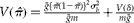 $$V \left ( \circ {>\pi } \right ) = \frac { \bar {>g} \left \{ \tilde {>\pi } (1 - \tilde {>\pi } )\right \}^{2} \sigma _{ b }^{2}}{ \bar {>g}m } + \frac { V ( \delta )}{ m\bar {>g} } $$
.
$$V \left ( \circ {>\pi } \right ) = \frac { \bar {>g} \left \{ \tilde {>\pi } (1 - \tilde {>\pi } )\right \}^{2} \sigma _{ b }^{2}}{ \bar {>g}m } + \frac { V ( \delta )}{ m\bar {>g} } $$
.
 $$\lambda $$
is the Lagrange multiplier. The partial derivatives of equation (14) with respect to
$$\lambda $$
is the Lagrange multiplier. The partial derivatives of equation (14) with respect to
 $$\lambda , m $$
and g are
$$\lambda , m $$
and g are
 $$\begin{eqnarray} \frac {\partial L }{\partial \lambda } = 0 = C - ( mgc _{1} + mc _{2});\ then\ m = \frac { C }{ c _{2} + gc _{1}} \end{eqnarray}$$
 $$\begin{eqnarray} \frac {\partial L }{\partial g } = 0 = - \frac { V ( \delta )}{ g ^{2} m } - \lambda mc _{1};\ then\ \lambda = - \frac { V ( \delta )}{ g ^{2} m ^{2} c _{1}} \end{eqnarray}$$
 $$\frac {\partial L }{\partial m } = 0 = - \frac {{\left \{ \tilde {>\pi } (1 - \tilde {>\pi } )}\right \}^{2} \sigma _{ b }^{2}}{ m ^{2}} - \frac { V \left ( \delta \right )}{ m ^{2} g } - \lambda [ gc _{1} + c _{2}] $$
 $$\begin{eqnarray} \Leftrightarrow \frac { V ( \delta )}{ g ^{2} m ^{2} c _{1}}[ gc _{1} + c _{2}] = \frac {{\left \{ \tilde {>\pi } (1 - \tilde {>\pi } )}\right \}^{2} \sigma _{ b }^{2}}{ m ^{2}} + \frac { V ( \delta )}{ m ^{2} g },\ since\ \lambda = - \frac { V ( \delta )}{ g ^{2} m ^{2} c _{1}} \end{eqnarray}$$
 $$\Leftrightarrow V \left ( \delta \right ) gc _{1} + V ( \delta ) c _{2} = g ^{2} c _{1}\left [\left \{ \tilde {>\pi } (1 - \tilde {>\pi } )\right \}^{2} \sigma _{ b }^{2} + \frac { V ( \delta )}{ g }\right ], $$
 $$\Leftrightarrow V ( \delta ) c _{2} = g ^{2} c _{1}\left \{{ \tilde {>\pi } (1 - \tilde {>\pi } )}\right \}^{2} \sigma _{ b }^{2} $$
 $$\begin{eqnarray} \Leftrightarrow g = \sqrt {\frac { c _{2}}{ c _{1}}}\frac {\sqrt { V ( \delta )}}{ \tilde {>\pi } (1 - \tilde {>\pi } ) \sigma _{ b }} \end{eqnarray}$$
Appendix B: Derivation of the optimal solution for minimizing
$$C = mgc _{1} + mc _{2} $$
subject to
$$V \left ( \circ {>\pi } \right ) = V _{0} $$


By combining equations (12) and (13), we obtain the Lagrangean
 $$\begin{eqnarray} L ( m , g , \lambda ) = L = mgc _{1} + mc _{2} + \lambda [ V \left ( \circ {>\pi } \right ) - V _{0}] \end{eqnarray}$$
where
 $$V \left ( \circ {>\pi } \right ) = \frac { \bar {>g} \left \{ \tilde {>\pi } (1 - \tilde {>\pi } )\right \}^{2} \sigma _{ b }^{2}}{ \bar {>g}m } + \frac { V ( \delta )}{ m\bar {>g} } $$
. Now the partial derivatives of L with respect to
$$V \left ( \circ {>\pi } \right ) = \frac { \bar {>g} \left \{ \tilde {>\pi } (1 - \tilde {>\pi } )\right \}^{2} \sigma _{ b }^{2}}{ \bar {>g}m } + \frac { V ( \delta )}{ m\bar {>g} } $$
. Now the partial derivatives of L with respect to
 $$\lambda , m $$
and g are
$$\lambda , m $$
and g are
 $$\begin{eqnarray} \frac {\partial L }{\partial \lambda } = 0 = \frac {{\left \{ \tilde {>\pi } (1 - \tilde {>\pi } )}\right \}^{2} \sigma _{ b }^{2}}{ m } + \frac { V ( \delta )}{ mg } - V _{0};\ then\ m = [\left \{ \tilde {>\pi } (1 - \tilde {>\pi } )\right \}^{2} \sigma _{ b }^{2} + \frac { V ( \delta )}{ g }]/ V _{0} \end{eqnarray}$$
 $$\frac {\partial L }{\partial g } = 0 = mc _{1} - \lambda \frac { V ( \delta )}{ g ^{2} m };\ then\ \lambda = \frac { g ^{2} m ^{2} c _{1}}{ V ( \delta )} $$
 $$\begin{eqnarray} \frac {\partial L }{\partial m } = 0 = gc _{1} + c _{2} - \frac { \lambda }{ m ^{2}}[\left \{{ \tilde {>\pi } (1 - \tilde {>\pi } )}\right \}^{2} \sigma _{ b }^{2} + \frac { V ( \delta )}{ g }] \end{eqnarray}$$
 $$\begin{eqnarray} \Leftrightarrow gc _{1} + c _{2} = \frac { g ^{2} m ^{2} c _{1}}{ V ( \delta )}\left [\frac {\left \{{ \tilde {>\pi } (1 - \tilde {>\pi } )}\right \}^{2} \sigma _{ b }^{2}}{ m ^{2}} + \frac { V ( \delta )}{ m ^{2} g }\right ],\ since\ \lambda = \frac { g ^{2} m ^{2} c _{1}}{ V ( \delta )} \end{eqnarray}$$
 $$\begin{eqnarray} \Leftrightarrow gc _{1} + c _{2} = \frac { g ^{2} c _{1}}{ V \left ( \delta \right )}\left [\left \{{ \tilde {>\pi } (1 - \tilde {>\pi } )}\right \}^{2} \sigma _{ b }^{2} + \frac { V ( \delta )}{ g }\right ], \end{eqnarray}$$
 $$\Leftrightarrow c _{2} = \frac { g ^{2} c _{1}}{ V \left ( \delta \right )}\left \{{ \tilde {>\pi } (1 - \tilde {>\pi } )}\right \}^{2} \sigma _{ b }^{2} $$
 $$\begin{eqnarray} \Leftrightarrow g = \sqrt {\frac { c _{2}}{ c _{1}}}\frac {\sqrt { V ( \delta )}}{ \tilde {>\pi } (1 - \tilde {>\pi } ) \sigma _{ b }}. \end{eqnarray}$$
Appendix C: Alternative derivation of the optimal solution for minimizing
$$C = mgc _{1} + mc _{2} $$
subject to
$$V \left ( \circ {>\pi } \right ) = V _{0} $$


If the sampling budget is C, the allocation of units as given in equation (15) results in a minimal value of
 $$V \left ( \circ {>\pi } \right ) $$
which in terms of cost is equal to:
$$V \left ( \circ {>\pi } \right ) $$
which in terms of cost is equal to:
 $$ V ( \circ {>\pi } ) = \frac { c _{2} + gc _{1}}{ C }\left [\left \{ \tilde {>\pi } (1 - \tilde {>\pi } )\right \}^{2} \sigma _{ b }^{2} + \frac { V ( \delta )}{ g }\right ] $$
where
 $$g = \sqrt {\frac { c _{2}}{ c _{1}}}\frac {\sqrt { V ( \delta )}}{ \tilde {>\pi } (1 - \tilde {>\pi } ) \sigma _{ b }} $$
. The solution to this problem can be derived directly since this budget C is also the minimal budget to obtain that particular value of
$$g = \sqrt {\frac { c _{2}}{ c _{1}}}\frac {\sqrt { V ( \delta )}}{ \tilde {>\pi } (1 - \tilde {>\pi } ) \sigma _{ b }} $$
. The solution to this problem can be derived directly since this budget C is also the minimal budget to obtain that particular value of
 $$V ( \circ {>\pi } ) $$
. If there were a smaller budget with other allocations yielding the same
$$V ( \circ {>\pi } ) $$
. If there were a smaller budget with other allocations yielding the same
 $$V ( \circ {>\pi } ) $$
, then our allocation (15) given C would not be optimal. This is true because the variable g appears in equation (C1) in the same manner as in equation (12), so that the
$$V ( \circ {>\pi } ) $$
, then our allocation (15) given C would not be optimal. This is true because the variable g appears in equation (C1) in the same manner as in equation (12), so that the
 $$g $$
of equation (15) is also the value of g which will minimize the cost of the sample if the variance of the estimate of the proportion (
$$g $$
of equation (15) is also the value of g which will minimize the cost of the sample if the variance of the estimate of the proportion (
 $$p ) $$
is fixed. Thus it also minimizes the cost variance product (Brooks, Reference Brooks1955). Thus, if a value of
$$p ) $$
is fixed. Thus it also minimizes the cost variance product (Brooks, Reference Brooks1955). Thus, if a value of
 $$V ( \circ {>\pi } ) $$
equal
$$V ( \circ {>\pi } ) $$
equal
 $$V _{0} = \omega ^{2} $$
/4
$$V _{0} = \omega ^{2} $$
/4
 $$Z _{1 - \alpha /2}^{2} $$
is required, the minimal budget to obtain this
$$Z _{1 - \alpha /2}^{2} $$
is required, the minimal budget to obtain this
 $$V ( \circ {>\pi } ) $$
follows by setting
$$V ( \circ {>\pi } ) $$
follows by setting
 $$V \left ( \circ {>\pi } \right ) $$
(as given in equation C1) equal to
$$V \left ( \circ {>\pi } \right ) $$
(as given in equation C1) equal to
 $$V _{0} = \omega ^{2} $$
/4
$$V _{0} = \omega ^{2} $$
/4
 $$Z _{1 - \alpha /2}^{2} $$
. Solving for budget C gives
$$Z _{1 - \alpha /2}^{2} $$
. Solving for budget C gives
 $$C = ( c _{2} + gc _{1})\left [\left \{ \tilde {>\pi } (1 - \tilde {>\pi } )\right \}^{2} \sigma _{ b }^{2} + \frac { V ( \delta )}{ g }\right ]/ V _{0} $$
and, finally, the corresponding optimal allocation of units follows from equation (15). Since
$$C = ( c _{2} + gc _{1})\left [\left \{ \tilde {>\pi } (1 - \tilde {>\pi } )\right \}^{2} \sigma _{ b }^{2} + \frac { V ( \delta )}{ g }\right ]/ V _{0} $$
and, finally, the corresponding optimal allocation of units follows from equation (15). Since
 $$m = \frac { C }{ c _{2} + gc _{1}} $$
and substituting
$$m = \frac { C }{ c _{2} + gc _{1}} $$
and substituting
 $$C = ( c _{2} + gc _{1})\left [\left \{ \tilde {>\pi } (1 - \tilde {>\pi } )\right \}^{2} \sigma _{ b }^{2} + \frac { V ( \delta )}{ g }\right ]/ V _{0} $$
, we obtain
$$C = ( c _{2} + gc _{1})\left [\left \{ \tilde {>\pi } (1 - \tilde {>\pi } )\right \}^{2} \sigma _{ b }^{2} + \frac { V ( \delta )}{ g }\right ]/ V _{0} $$
, we obtain
 $$m = [\left \{{ \tilde {>\pi } (1 - \tilde {>\pi } )}\right \}^{2} \sigma _{ b }^{2} $$
+
$$m = [\left \{{ \tilde {>\pi } (1 - \tilde {>\pi } )}\right \}^{2} \sigma _{ b }^{2} $$
+
 $$\frac { V ( \delta )}{ g }]/ V _{0} $$
and
$$\frac { V ( \delta )}{ g }]/ V _{0} $$
and
 $$g = \sqrt {\frac { c _{2}}{ c _{1}}}\frac {\sqrt { V ( \delta )}}{ \tilde {>\pi } (1 - \tilde {>\pi } ) \sigma _{ b }} $$
.
$$g = \sqrt {\frac { c _{2}}{ c _{1}}}\frac {\sqrt { V ( \delta )}}{ \tilde {>\pi } (1 - \tilde {>\pi } ) \sigma _{ b }} $$
.
Appendix D: Taylor series approximation (equation 23) of the RE in equation (21) given by Van Breukelen et al. (Reference Van Breukelen, Candel and Berger2007)
Taylor series approximation (equation 23) is derived from the RE of equation (21) in four steps.
Step 1
Let the
 $$g _{ i } $$
values be independent realizations of a random variable cluster size U with expectation
$$g _{ i } $$
values be independent realizations of a random variable cluster size U with expectation
 $$\mu _{ n } $$
and standard deviation
$$\mu _{ n } $$
and standard deviation
 $$\mu _{ n } $$
. Equation (19) is a moment estimator of
$$\mu _{ n } $$
. Equation (19) is a moment estimator of
 $$ RE \left ( \circ {>\pi } \right ) = \frac { \bar {>g} + \alpha }{ \bar {>g} } E \left (\frac { U }{ U + \alpha }\right ) $$
where
 $$\alpha = (1 - \rho )/ \rho \geq 0 $$
.
$$\alpha = (1 - \rho )/ \rho \geq 0 $$
.
Step 2
Define
 $$d = \left ( U - \mu _{ n }\right ) $$
; then the last term in equation (D1) can be written as:
$$d = \left ( U - \mu _{ n }\right ) $$
; then the last term in equation (D1) can be written as:
 $$\begin{eqnarray} E \left (\frac { U }{ U + \alpha }\right ) = E \left (\frac { \mu _{ n } + d }{ \mu _{ n } + \alpha + d }\right ) = E \left \{\left (\frac { \mu _{ n } + d }{ \mu _{ n } + \alpha }\right )\left (\frac {1}{1 + ( d /( \mu _{ n } + \alpha ))}\right )\right \}. \end{eqnarray}$$
The last term is a Taylor series [Mood et al. (Reference Mood, Graybill and Boes1974), p. 533, equation 34]:
 $$\begin{eqnarray} \left (\frac {1}{1 + ( d /( \mu _{ n } + \alpha ))}\right ) = { \sum _{ j = 0}^{\infty } }\,(\frac { - d }{ \mu _{ n } + \alpha })^{ j } \end{eqnarray}$$
if
 $$- \left ( \mu _{ n } + \alpha \right )\lt d \lt \left ( \mu _{ n } + \alpha \right ) $$
to ensure convergence.
$$- \left ( \mu _{ n } + \alpha \right )\lt d \lt \left ( \mu _{ n } + \alpha \right ) $$
to ensure convergence.
Since
 $$d = U - \mu _{ n } $$
and
$$d = U - \mu _{ n } $$
and
 $$\alpha \geq 0 $$
, this convergence condition will be satisfied, except for a small probability
$$\alpha \geq 0 $$
, this convergence condition will be satisfied, except for a small probability
 $$P ( U > 2 \mu _{ n } + \alpha ) $$
for strongly positively skewed cluster size distributions combined with large
$$P ( U > 2 \mu _{ n } + \alpha ) $$
for strongly positively skewed cluster size distributions combined with large
 $$\rho ( = small \alpha ) $$
. Thus we have:
$$\rho ( = small \alpha ) $$
. Thus we have:
 $$ E \left (\frac { U }{ U + \alpha }\right ) = E \left \{\left (\frac { \mu _{ n } + d }{ \mu _{ n } + \alpha }\right ){ \sum _{ j = 0}^{\infty } }\,\left (\frac { - d }{ \mu _{ n } + \alpha }\right )^{ j }\right \}. $$
Step 3
If we ignore all terms
 $$d ^{ j } $$
with
$$d ^{ j } $$
with
 $$j > 2 $$
and rearrange terms in equation (D2), we will have
$$j > 2 $$
and rearrange terms in equation (D2), we will have
 $$ E \left (\frac { U }{ U + \alpha }\right ) = \lambda \left \{{1 - CV ^{2} \lambda \left (1 - \lambda \right )}\right \} $$
where
 $$\lambda = ( \mu _{ g }/( \mu _{ g } + \alpha ))\in (0,1] $$
, assuming
$$\lambda = ( \mu _{ g }/( \mu _{ g } + \alpha ))\in (0,1] $$
, assuming
 $$\bar {>g} = \mu _{ g } $$
and
$$\bar {>g} = \mu _{ g } $$
and
 $$CV = \sigma _{ g }/ \mu _{ g } $$
is the coefficient of variation of the random variable U.
$$CV = \sigma _{ g }/ \mu _{ g } $$
is the coefficient of variation of the random variable U.
Step 4
Plugging (D3) into (D1) gives:
 $$ RE \left ( \circ {>\pi } \right )_{ t }\approx \left \{1 - CV ^{2} \lambda \left (1 - \lambda \right )\right \}. $$
Remark
Ignoring in (D2) only those
 $$d ^{ j } $$
terms with
$$d ^{ j } $$
terms with
 $$j > 4 $$
instead of 2 will give
$$j > 4 $$
instead of 2 will give
 $$ RE \left ( \circ {>\pi } \right )_{ t }\approx 1 - \left \{{(1 - \lambda )[ \lambda CV ^{2} - \lambda CV ^{3}skew + \lambda ^{3} CV ^{4}\left (kurt + 3\right )]}\right \} $$
where skew and kurt are the skewness and kurtosis of the cluster size distribution, that is, skew = the third central moment of the U divided by
 $$\sigma _{ n }^{3} $$
, and kurt = the fourth moment of U divided by
$$\sigma _{ n }^{3} $$
, and kurt = the fourth moment of U divided by
 $$\sigma _{ n }^{4} $$
, minus 3 (see, for example, Mood et al., Reference Mood, Graybill and Boes1974, p. 76).
$$\sigma _{ n }^{4} $$
, minus 3 (see, for example, Mood et al., Reference Mood, Graybill and Boes1974, p. 76).


 Open access