


1. INTRODUCTION
Although many researchers nowadays mostly focus on Global Navigation Satellite System (GNSS) positioning, navigation and timing technique (e.g. Montenbruck et al., Reference Montenbruck, Steigenberger, Khachikyan, Weber, Langley, Mervart and Hugentobler2014; Li et al., Reference Li, Zhang, Ren, Fritsche, Wickert and Schuh2015a), velocity estimation still plays an important role in many fields, such as airborne gravimetry, precision agriculture, Rendezvous Docking of aircraft, etc. High-precision velocity estimation using a stand-alone receiver from Global Position System (GPS) broadcast ephemeris has been introduced in many studies (Hebert et al., Reference Hebert, Keith, Ryan, Szarmes, Lachapelle and Cannon1997; Bruton et al., Reference Bruton, Glennie and Schwarz1999; Serrano et al., Reference Serrano, Kim and Langley2004a; Van Graas and Soloviev, Reference Van and Soloviev2004; Ding and Wang, Reference Ding and Wang2011; Wang and Xu, Reference Wang and Xu2011; Zhang, Reference Zhang2007). The results show that the accuracy of velocity estimation with carrier-phase-derived Doppler in a static mode can reach a few mm/s and a few cm/s in a kinematic mode.
The Chinese BeiDou Navigation Satellite System (BDS) is now providing continuous Positioning, Navigation and Timing (PNT) services to the Asian-Pacific area. By the end of 2014, 16 BDS satellites were launched, which formed a regional positioning system. 14 satellites are in operation, including five Geosynchronous Orbit (GEO) satellites, five Inclined Geosynchronous Orbit (IGSO) satellites, and four Medium Earth Orbit (MEO) satellites (Li et al., Reference Li, Ge, Dai, Ren, Fritsche, Wickert and Schuh2015b). China plans to launch upgraded satellites and expand its regional BDS to global coverage by 2020 (Yang et al., Reference Yang, Li, Wang, Xu, He, Guo, Shen and Dai2014), so it is necessary and important to evaluate the performance of velocity estimation with BDS satellites.
Generally there are two ways to obtain satellites’ velocity: the position-derivation method and the analytic method (by differentiating the position formulae). We compare the results of both methods with the velocity estimation calculated from precise ephemeris using first-order central difference of a Taylor series approximation and find that both methods deliver better than 1 mm/s velocity estimation from GPS broadcast ephemeris (Zhang et al., Reference Zhang, Zhang, Grenfell and Deakin2006; Serrano et al., Reference Serrano, Kim and Langley2004a). Nevertheless, we still need to investigate whether these methods can achieve the same performance in BDS. Since the algorithm for IGSO/MEO is the same as GPS, here we just focus on the GEO satellite velocity determination.
As we know, troposphere delay and ionosphere delay are the main error sources in the velocity estimation. Some scholars consider these two errors were highly time correlated and could be mitigated over a short time interval (less than or equal to two seconds) (Ding and Wang, Reference Ding and Wang2011; Serrano et al., Reference Serrano, Kim and Langley2004a; Zhang and Li, Reference Zhang and Li2012; Li et al., Reference Li, Zhang and Guo2014), thus only single-frequency observations are used. However, the ionosphere can be very active and the slant ionospheric delay at lower elevation angle may change significantly, which could decrease the accuracy of velocity estimation. To eliminate this influence, ionosphere-free combination observation (LC) was employed (Van and Soloviev, Reference Van and Soloviev2004; Kennedy, Reference Kennedy2003; Ge et al., Reference Ge, Gendt, Rothacher, Shi and Liu2008; Li and Zhang, Reference Li and Zhang2012). So far, no results of comparison of these two methods have been published to our knowledge.
Additionally, for a single navigation system, both precision and reliability will deteriorate rapidly in certain environments such as in urban canyons or in mountainous regions where there are insufficient visible satellites. However, this shortage can be compensated by using combined GNSS constellations, which could significantly improve the geometry of observed satellites (Li et al., Reference Li, Ge, Dai, Ren, Fritsche, Wickert and Schuh2015b), and thus improve the precision of velocity estimation as well as its reliability and availability. For multi-systems data processing, precise weighting of the observations from different systems is very important because the measurements of different systems have different noise level and residual errors. To find the proper weights of observations, the Helmert Variance Component Estimation (HVCE) has been widely used (Cai et al., Reference Cai, Pan and Gao2014; Koch, Reference Koch1999). However, this requires a longer time to iterate, high redundant observations, and is not available for real-time application. In order to enhance calculation efficiency, an a priori weight ratio method has more potential.
This paper assesses the performance of velocity estimation using single BDS and combined GPS/BDS in both static and kinematic modes. A poor observation environment will be simulated in static test. Before velocity estimation, the algorithms for real-time BDS GEO satellite Earth-Centred-Earth-Fixed (ECEF) velocity estimation will be presented, then compared with a position-derivation method. The accuracy of satellite position estimation and clock drift estimation from BDS broadcast ephemeris will also be analysed. The results using both single- and dual-frequency are shown in order to investigate the influence of ionospheric error on velocity estimation. Finally a comparison of HVCE and an a priori weight ratio method will be demonstrated.
2. GPS/BDS VELOCITY ESTIMATION PROCEDURES
Velocity can be obtained by carrier-phase-derived Doppler (Kennedy et al., Reference Kennedy2003; Serrano, Reference Serrano, Kim, Langley, Itani and Ueno2004b). Considering the observation equation for BDS is similar to that of GPS, only the combined GPS/BDS observation equation is given here:
 $${\dot \varphi}_u^{s} = {e_u^{s} \cdot} ({\dot {\vec {\rm r}}}^{s} - {\dot{\vec {\rm r}}}_{u}) + {c \cdot} {\dot {t_{G,u}}} + {c \cdot} {\dot {t_{{\rm B},u}}} - {c \cdot} {\dot t}^{s} + {\dot T}_u^{s} + {\dot I}_u^{s} + \varepsilon $$
 $$e_u^{s} = \displaystyle{{{\vec {\rm r}^{s}} - {\vec {\rm r}_u}} \over {{\rho _u}}}$$
 $${\rho _u} = \left\vert {{\vec r}^s + c \cdot {\dot t}^s - ({\vec r}_u + c \cdot {\dot t}_u)} \right\vert $$ ${dot \varphi} $ represents the Doppler measurements, $e_u^s$ the directional cosine, ρ uthe geometric distance between receiver u and satellite s, ${\dot{\vec {\rm r}}}^{s}$ the satellite velocity vector, ${\dot {\vec {\rm r}}}_u$ the receiver velocity vectors, c the speed of light in a vacuum, ${\dot t}_u$ ( ${\dot t}_{G,u}$ and ${\dot t}_{{\rm B},u}$) the receiver clock drift parameters for GPS and BDS, respectively, ${\dot t}^s$ the satellite clock drift (Zhang et al., Reference Zhang, Li and Guo2011), ${\dot I}$, ${\dot T}$ the ionospheric and tropospheric delay rate respectively, ε the measurements noise.
To reduce the effect of tropospheric delay and ionospheric delay in the observation, the Saastamoinen model (Saastamoinen, Reference Saastamoinen1973) and the ionosphere-free combination observation (LC) (Ge et al., Reference Ge, Gendt, Rothacher, Shi and Liu2008) are employed. As to the stochastic model, we assume that the noise is dependent on elevation, so the sine function of the elevation angle is employed (King and Bock, Reference King and Bock1999). The cut-off angle is set to 15° if there is no special introduction. Since GPS and BDS carrier phase observations have the same level of precision (Yang et al., Reference Yang, Li, Wang, Xu, He, Guo, Shen and Dai2014; Li et al., Reference Li, Zhang, Ren, Fritsche, Wickert and Schuh2015a), we adopt Equivalent Weight Ratio (EWR) in the process of the combined observations and assume the observations are independent. When all errors are modelled or negligible, we can describe the unknown parameters as  ${X_v} = [{\dot {\vec {\rm r}}}_u {\dot t}_{G,u} {\dot t}_{B,u}]$ in the Least Square adjustment.
3. THE BDS BROADCAST EPHEMERIS ANALYSIS
According to Equation (1), it can be seen that high-precision velocity estimation not only depends on the accuracy of the measurements, but also depends on the accuracy of satellite position, velocity, clock drift calculated from the broadcast ephemeris and the accuracy of Single Point Positioning (SPP). These effects have been analysed for GPS (Zhang, Reference Zhang2007). However, only a few research efforts focus on these effects for BDS. Yang et al. (Reference Yang, Li, Wang, Xu, He, Guo, Shen and Dai2014) show that the accuracy of SPP in BDS is better than 10 m in the Asia-Pacific region, which is in the same level of magnitude to that of GPS. In this consideration, the positioning error can be ignored. Thus, it is meaningful to make a comprehensive analysis of BDS broadcast ephemeris.
An algorithm for BDS satellite ECEF position and satellite clock drift from the broadcast ephemeris is presented in the BeiDou-ICD-2·0-2013 (CSNO, 2013). Satellite velocity can be obtained from position differential and closed-form formulae. Since the algorithm for IGSO/MEO is the same as that of GPS, we just give the GEO satellite velocity closed-form formula according to the position algorithm.
GEO satellite position in ECEF can be expressed as (CSNO, 2013):
 $${\left[ {\matrix{ X \cr Y \cr Z \cr}} \right]_{ECEF}} = {R_Z}(\omega {t_k}){R_X}( - {5^{\circ}} )R\left[ {\matrix{ x \cr y \cr 0 \cr}} \right]$$
where:
 $$\eqalign{R & = \left[ {\matrix{ {\cos L} & { - \sin L\cos I} & {\sin L\sin I} \cr {\sin L} & {\cos L\cos I} & { - \cos L\sin I} \cr 0 & {\sin I} & {\cos I} \cr}} \right]\!,{R_Z}(\omega {t_k}) \cr & = \left[ {\matrix{ {\cos (\omega {t_k})} & {\sin (\omega {t_k})} & 0 \cr { - \sin (\omega {t_k})} & {\cos (\omega {t_k})} & 0 \cr 0 & 0 & 1 \cr}} \right]\!,{R_X}( - {5^{\circ}} ) = \left[ {\matrix{ 1 & 0 & 0 \cr 0 & {\cos {5^{\circ}}} & {\sin {5^{\circ}}} \cr 0 & { - \sin {5^{\circ}}} & {\cos {5^{\circ}}} \cr}} \right]}$$
(x, y, 0) denotes the satellite position in the natural orbit plane system, L the longitude of the ascending node, I the orbit inclination, ω the earth rotation parameter, t k the interval between time of observation and reference ephemeris.
The satellite velocity vector ( ${\dot X} $, ${\dot Y} $, ${\dot Z} $) can be obtained by taking the derivative of the satellite position:
 $$\eqalign{\left[ {\matrix{ {\dot X} \cr {\dot Y} \cr {\dot Z} \cr}} \right] & = {\dot R}_Z(\omega {t_k}){R_X}( - {5^{\circ}} )R\left[ {\matrix{ x \cr y \cr 0 \cr}} \right] + {R_Z}(\omega {t_k}){R_X}( - {5^{\circ}} ){\dot R}\left[ {\matrix{ x \cr y \cr 0 \cr}} \right] \cr & + {R_Z}(\omega {t_k}){R_X}( - {5^{\circ}} )R\left[ {\matrix{ {\dot x} \cr {\dot y} \cr 0 \cr}} \right]}$$
 $$\eqalign{& {{\dot R}_Z}(\omega {t_k}) = \left[ {\matrix{ { - \omega \sin (\omega {t_k})} & {\omega \cos (\omega {t_k})} & 0 \cr { - \omega \cos (\omega {t_k})} & { - \omega \sin (\omega {t_k})} & 0 \cr 0 & 0 & 0 \cr}} \right]\!, \cr & {\dot R} = \left[ {\matrix{ { - {\dot L}\sin L} & { - {\dot L}\cos L\cos I + {\dot I}\sin L\sin I} & {{\dot L}\cos L\sin I + {\dot I}\sin L\cos I} \cr {{\dot L}\cos L} & { - {\dot L}\sin L\cos I - {\dot I}\cos L\sin I} & {{\dot L}\sin L\sin I - {\dot I}\cos L\cos I} \cr 0 & {{\dot I}\cos I} & { - {\dot I}\sin I} \cr}} \right]} $$
where the dot represents the first derivative with respect to time.
Figure 1 shows that the residuals of the satellite 3D velocity for C03(GEO), C06(IGSO), C14(MEO) from the differentiation method are better than the closed-form formula: although manifesting systematic bias, its precision is better than 1 mm/s. The main explanations are as follow: (1) Orbit errors are absorbed into velocity parameters when we use the analytic method directly. (2) Due to the high stability of the satellite orbit, the satellite position error even up to 10 m can be suppressed by differentiation. Figure 2 depicts the accuracy of satellite positions and clock drifts calculated from BDS broadcast ephemeris. Obviously, it can meet the demands of high-precision velocity estimation.

Figure 1. Residuals of satellite velocity obtained from the closed-form formula (a) and position-derivation (b) compared with the velocity obtained from the SP3 precise ephemeris using first-order central difference of a Taylor series approximation (PRN = C03/C06/C14,15:30:00~16:30:00, 10/01/2014).

Figure 2. Proof that the satellite position and clock drift calculated by using the broadcast ephemeris is sufficiently accurate in comparison with SP3 precise ephemeris (PRN = C03/C06/C14,15:30:00~16:30:00, 10/01/2014).
4. STATIC TEST
In order to assess the performance of stand-alone velocity estimation for GPS/BDS comprehensively, three experiment schemes were designed: scheme1 single-frequency (SF) (B1, L1), scheme2, LC with cut-off angle 15°, 30° and 45°, scheme3 LC (B1/B2, L1/L2) with HVCE method. Dual-frequency GPS/BDS data sets from eight stations (WHCD, WHDH, WHEZ, WHHN, WHHP, WHKC, WHQJ, WHXT) at the Wuhan CORS on 1 October 2014 were collected with sampling interval of 1s. Since true velocity is zero, the test results would help to reveal the sources and characteristics of estimation error.
Take the station WHCD as an example, the sky plots of GPS and BDS satellites are shown in Figure 3, and the corresponding dilution of precision in horizontal (HDOP) and vertical (VDOP) directions are given in Figure 4. It can be seen that, compared with a GPS-only system, the mean HDOP, VDOP of integrated GPS/BDS increased nearly 30% and 33%. This means the geometry is significantly improved in the integrated GPS/BDS. As for BDS, the HDOP and VDOP are worse than GPS because the satellites distribution is incomplete.

Figure 3. Sky plots of BDS (left) and GPS (right) satellites of station WHCD. The purple lines represent observations with B1/B2 frequencies, the green lines represent observations with L1/L2 frequencies, and the yellow lines represent observations with L1 frequency only.

Figure 4. HDOP, VDOP of GPS, BDS and GPS/BDS (station: WHDH).
The ionospheric error is a vital error source in data processing (Li et al., Reference Li, Ge, Zhang and Wickert2013). Comparing Figure 5 (scheme1) and Figure 7 (scheme2), we can see that many fluctuations occur in the three components of velocity estimation for GPS, especially during the GPS Second 280000~294000 (in the red rectangle box), while for BDS, there is only a small difference. The reason is that the ionospheric delay change rates along the signal transmitting path of GEO satellites are slower than that of IGSO, MEO satellites. This is due to the fact that GEO satellites are stationary with respect to the earth, thus the impact of ionospheric delay on velocity estimation in BDS is less than that of GPS. Besides, LC combinations are preferred in active ionosphere environments, such as ionospheric disturbance.

Figure 5. Scheme1 velocity estimation using SF for East/North/Up components (station: WHCD).
The precision statistics based on the results of these eight stations are illustrated in Figure 6. Obviously, the accuracy of North and East components are better than the Up component. The Root Mean Square (RMS) and mean value of BDS are already comparable to GPS, where the mean value is nearly 0·0 in the horizontal component and 1 mm/s in the vertical component, the RMS is better than 2 mm/s in the horizontal and within 5 mm/s in the upward component. Compared to a GPS-only system, the RMSs of the combined system improves 14%, 23% and 24% in East/North/Up components respectively, and the advantage will be more remarkable in challenging environments.

Figure 6. The precision statistics of velocity estimation for GPS, BDS and GPS/BDS using LC from 8 stations.
To simulate poor observation conditions, we design scheme 2 and the results are depicted in Figure 7, Figure 8, and Figure 9. From Table 1, we can see that with cut-off angle increasing, the number of visible satellites decreases rapidly, and the geometry strength becomes weaker, consequently, the accuracy as well as reliability of velocity estimation decreases. Furthermore, for GPS/BDS, the Percentage of Valid Epochs (PVE) which can be used in the calculation still reaches 97% during the test, which quite outnumbers that of the single system.

Figure 7. Scheme2 Velocity estimation using LC for East/North/Up components with cut-off angle 15°(station: WHCD).

Figure 8. Scheme2 Velocity estimation using LC for East/North/Up components with cut-off angle 30°(station: WHCD).

Figure 9. Scheme2 Velocity estimation using LC for East/North/Up components with the cut-off angle 45°(station: WHCD).
Table 1. Percentage of valid epochs and corresponding visible satellite number.

Table 2 illustrates the precision statistics of scheme2 (cut-off angle 15°) and scheme3, in respect of precision statistics, they are mostly consistent. Furthermore, the program running time improves almost 25% by the EWR method. To further verify the applicability and reliability of EWR, the variance ratios of GPS/BDS from HVCE are calculated. These values are ranges from 0·7 to 1·5. Their mean value is 1·13, and RMS is 1·18.These show the EWR is well supported.
Table 2. Statistic and program running time of stand-alone velocity estimation using HVCE and EWR.

5. KINEMATIC TEST
The implemented kinematic test was carried out in Jiangxia District, Wuhan, on 7 June 2014. Dual frequency carrier phase measurements were collected using a South-GNSS-S82C receiver with a sampling interval of 1s. The rover receiver was mounted on a car and its trajectory is shown in Figure 10. The number of satellites tracked is shown in Figure 11. The base receiver was installed on an open site. Since it is very difficult to obtain true velocity in a kinematic test, in our case, we use the reference velocity that was derived through numerical differentiation of the receiver positions that were processed by post processing Differential GPS techniques (DGPS) (Ding and Wang, Reference Ding and Wang2011) with a commercial software tool, i.e. GrafNav, shown in Figure 12.

Figure 10. The car's ground track.
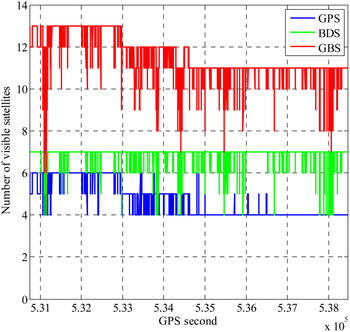
Figure 11. Number of the tracked satellites during the test.

Figure 12. Velocity obtained from DGPS with first-order central difference of a Taylor series approximation. These three panels illustrate East, North and Up components of the velocity.
Figure 13 depicts 3D velocity difference between the stand-alone velocity solution and that of DGPS, wherein the results calculated by HVCE are marked with ‘*’. It can be seen that the residual noise of BDS is at the same level of magnitude as that of GPS in the horizontal component but worse in the Up component, and for GPS/BDS, the residual noise is the least. From Table 3, we can see that the number of valid epochs for GPS is less than BDS and GPS/BDS. The reason is that some GPS satellites signal were obscured during the test, while there were five BDS satellites at high-elevation angles above 30°. Although HVCE is a rigorous weighting approach, which requires high redundant observations, these could not be always satisfied in poor observation conditions, thus resulting in unreliable weight solutions and low reliability of velocity estimation. The EWR works quite well, considering its mean value of residuals shown above appear to be unbiased, its RMS of horizontal component is below 0·3 cm/s and its RMS of the upward component is nearly 1 cm/s. Above all the results of the kinematic test agree with the former static test very well.

Figure 13. The 3D velocity difference between the stand alone velocity solution and the reference velocity.
Table 3. Accuracy and valid epochs statistics of stand-alone velocity.

6. CONCLUSIONS
In this paper, we evaluated the performance of velocity estimation of the BDS as well as the integrated GPS/BDS. The conclusions are as follows:
Compared with position-derivation method from precise ephemeris SP3, the BDS satellite velocity using position-derivation method whose accuracy is above 1 mm/s is better than closed-form formulae from broadcast ephemeris. In addition it simplifies the velocity transformation procedure, and provides a good alternative. Both the satellite position and clock drift obtained from BDS broadcast ephemeris meet the demands of high precision velocity estimation.
When the satellite geometry distribution is similar, the results of BDS are comparable to GPS, and its stability and accuracy noticeably improve in the integrated GPS/BDS, especially under poor observation conditions.
Compared with LC, the SF can be influenced by ionosphere delay, which can cause errors as much as 1~2 cm/s, thus we prefer LC in practice.
It is appropriate and applicable to use a prior weight, i.e. EWR in processing the GPS/BDS combined observations, whose performance is at the same level of magnitude or even better than that of HVCE which is limited by redundant observations, and because there is no need of iteration, the EWR is more efficient.
ACKNOWLEDGEMENTS
This work is supported by the Natural Science Foundation for Distinguished Young Scholar of Hubei Province (No: 2015CFA039) and the Spark Program of Earthquake Sciences (No. XH16053).


