


Introduction
Airborne electromagnetics (AEM) is an effective technique to investigate the shallow subsurface. It has successfully been applied in various geological settings to analyse the depositional architecture (e.g. Jordan & Siemon, Reference Jordan and Siemon2002; Huuse et al., Reference Huuse, Piotrowski and Lykke-Andersen2003; Sandersen & Jørgensen, Reference Sandersen and Jørgensen2003; Paine & Minty, Reference Paine, Minty, Rubin and Hubbard2005; Jørgensen & Sandersen, Reference Jørgensen and Sandersen2006, Reference Jørgensen and Sandersen2009; Bosch et al., Reference Bosch, Bakker, Gunnink and Paap2009; Steuer et al., Reference Steuer, Siemon and Auken2009; Pryet et al., Reference Pryet, Ramm, Chilès, Auken, Deffontaines and Violette2011; Burschil et al., Reference Burschil, Wiederhold and Auken2012a,Reference Burschil, Scheer, Kirsch and Wiederholdb; Klimke et al., Reference Klimke, Wiederhold, Winsemann, Ertl and Elbracht2013). AEM enables a fast geological overview mapping of subsurface structures and allows different lithologies and pore water conditions to be distinguished (Siemon, Reference Siemon2005; de Louw et al., Reference de Louw, Eeman, Siemon, Voortman, Gunnink, van Baaren and Oude Essink2011; Burschil et al., Reference Burschil, Wiederhold and Auken2012a). Inversion procedures are carried out to create resistivity-depth models (e.g. Siemon et al., Reference Siemon, Christiansen and Auken2009a,Reference Siemon, Auken and Christiansenb), which are the basis for resistivity-depth sections and maps. Although this technique is a well-established method to improve geological interpretations of the subsurface architecture, there is a substantial need for an efficient and reliable methodology to image the results in three dimensions.
Progress in imaging the results in three dimensions was made by combining 1D inversion models into 3D gridded data models (e.g. Lane et al., Reference Lane, Green, Golding, Owers, Pik, Plunkett, Sattel and Thorn2000; Jørgensen et al., Reference Jørgensen, Sandersen, Auken, Lykke-Andersen and Sørensen2005; Bosch et al., Reference Bosch, Bakker, Gunnink and Paap2009; Palamara et al., Reference Palamara, Rodriguez, Kellett and Macaulay2010; Jørgensen et al., Reference Jørgensen, Rønde Møller, Nebel, Jensen, Christiansen and Sandersen2013). However, this integration gave limited consideration to uncertainties related to the interpolation procedure (e.g. Pryet et al., Reference Pryet, Ramm, Chilès, Auken, Deffontaines and Violette2011). To minimise these uncertainties different approaches were developed, including an integrated geophysical and geological interpretation based on AEM surveys, reflection seismic sections, borehole data and logs. This provides the most reliable results and leads to a minimisation of interpretational uncertainties (e.g. Gabriel et al., Reference Gabriel, Kirsch, Siemon and Wiederhold2003; Jørgensen et al., Reference Jørgensen, Lykke-Andersen, Sandersen, Auken and Nørmark2003a; BurVal Working Group, 2009; Jørgensen & Sandersen, Reference Jørgensen and Sandersen2009; Høyer et al., Reference Høyer, Lykke-Andersen, Jørgensen and Auken2011; Jørgensen et al., Reference Jørgensen, Rønde Møller, Nebel, Jensen, Christiansen and Sandersen2013). However, little attention has been paid to developing methodologies with an integrated interpretation using different geological and geophysical data sets for the shallow subsurface.
The aim of this paper is to provide a methodology to construct a 3D subsurface model with reduced interpretation uncertainties by integrating AEM, borehole and seismic data. The method was applied and tested with data sets 6 km south from Cuxhaven, northwest Germany. The study area comprises Neogene sediments that are incised by an Elsterian tunnel valley. Previous studies focused on overview mapping of Neogene and Palaeogene marker horizons and Pleistocene tunnel valleys from 2D reflection seismic sections and borehole logs (Gabriel et al., Reference Gabriel, Kirsch, Siemon and Wiederhold2003; BurVal Working Group, 2009; Rumpel et al., Reference Rumpel, Binot, Gabriel, Siemon, Steuer and Wiederhold2009). Larger conductive structures within the valley fill were identified from 1D inversion results of frequency-domain helicopter-borne electromagnetic data (HFEM) and time-domain helicopter-borne electromagnetic data (HTEM) inversion results (Rumpel et al., Reference Rumpel, Binot, Gabriel, Siemon, Steuer and Wiederhold2009; Steuer et al., Reference Steuer, Siemon and Auken2009). Using the previous results and interpretations as well as our new data sets, we provide a detailed analysis of the seismic facies and sedimentary systems included in a 3D geological subsurface model, resolving architectural elements in much greater detail. We generated 3D resistivity grids based on the geostatistical analysis and interpolation of 1D AEM inversion results. The 3D resistivity grids combine the advantage of volumetric computations with the visualisation of wide resistivity ranges and allow the direct comparison and implementation of additional data sets such as borehole and seismic data to improve the geological interpretation of the shallow subsurface.
Geological setting and previous research
The study area is 7.5 km by 7.5 km and is located in northwest Germany, between Cuxhaven in the north and Bremerhaven in the south (Fig. 1A). The study area belongs to the Central European Basin System that evolved from the Variscan foreland basin in the Late Carboniferous (Betz et al., Reference Betz, Führer, Greiner and Plein1987).

Fig. 1. (A) Location of the study area and maximum extent of the Pleistocene ice sheets (modified after Jaritz, 1987; Baldschuhn et al., Reference Baldschuhn, Frisch and Kockel1996, Reference Baldschuhn, Binot, Fleig and Kockel2001; Scheck-Wenderoth & Lamarche, Reference Scheck-Wenderoth and Lamarche2005; Ehlers et al., Reference Ehlers, Grube, Stephan, Wansa, Ehlers, Gibbard and Hughes2011). (B) Hill-shaded relief model of the study area, showing the outline of the Hohe Lieth ridge. (C) Close-up view of the study area showing the location of Pleistocene tunnel valleys (light yellow) and the location of boreholes (coloured dots). Boreholes used in the seismic and cross-sections are indicated by larger dots; seismic sections S1 (Fig. 4), S2 and S3 (Fig. 5) are displayed as black lines. Cross-section A–B is visualised in Fig. 6; C–D is visualised in Fig. 7. (D) HFEM surveys are displayed as grey lines; HTEM surveys are displayed as dark grey dots.
In Permian times a wide continental rift system developed, resulting in N–S trending graben structures (Gast & Gundlach, Reference Gast and Gundlach2006). During the Late Permian, repeated marine transgressions flooded the subbasins and thick evaporite successions formed (Pharaoh et al., Reference Pharaoh, Dusar, Geluk, Kockel, Krawczyk, Krzywiec, Scheck-Wenderoth, Thybo, Vejbæk, Wees, van, Doornenbal and Stevenson2010). Extensional tectonics during the Middle to Late Triassic led to the formation of NNE–SSW trending graben structures, following the orientation of major basement faults. The main extensional phase in the Late Triassic was accompanied by strong salt tectonics and rim-syncline development (Kockel, Reference Kockel2002; Grassmann et al., Reference Grassmann, Cramer, Delisle, Messner and Winsemann2005; Maystrenko et al., Reference Maystrenko, Bayer and Scheck-Wenderoth2005a). During the Late Cretaceous to Early Palaeogene, the area was tectonically reactivated, an event that is related to the Alpine Orogeny (Maystrenko et al., Reference Maystrenko, Bayer and Scheck-Wenderoth2005a) and was accompanied by local subsidence and ongoing salt tectonics (Baldschuhn et al., Reference Baldschuhn, Frisch and Kockel1996, Reference Baldschuhn, Binot, Fleig and Kockel2001; Kockel, Reference Kockel2002; Grassmann et al., Reference Grassmann, Cramer, Delisle, Messner and Winsemann2005; Maystrenko et al., Reference Maystrenko, Bayer and Scheck-Wenderoth2005a; Rasmussen et al., Reference Rasmussen, Dybkjær and Piasecki2010).
Palaeogene and Neogene marginal-marine deposits
Since the Late Oligocene, sedimentation in the North Sea Basin has been dominated by a large clastic depositional system, fed by the Baltic River System (Huuse & Clausen, Reference Huuse and Clausen2001; Overeem et al., Reference Overeem, Weltje, Bishop-Kay and Kroonenberg2001; Huuse, Reference Huuse2002; Kuster, Reference Kuster2005; Møller et al., Reference Møller, Rasmussen and Clausen2009; Knox et al., Reference Knox, Bosch, Rasmussen, Heilmann-Clausen, Hiss, De Lugt, Kasińksi, King, Köthe, Słodkowska, Standke, Vandenberghe, Doornenbal and Stevenson2010; Anell et al., Reference Anell, Thybo and Rasmussen2012; Rasmussen & Dybkjær, Reference Rasmussen and Dybkjær2013; Thöle et al., Reference Thöle, Gaedicke, Kuhlmann and Reinhardt2014). Initially the Baltic River System, draining the Fennoscandian Shield and the Baltic Platform, prograded from the northeast, and then the sediment transportation direction rotated clockwise to southeast (Sørensen et al., Reference Sørensen, Gregersen, Breiner and Michelsen1997; Michelsen et al., Reference Michelsen, Thomsen, Danielsen, Heilmann-Clausen, Jordt, Laursen, Graciansky, Hardenbol, Jacquin and Vail1998; Huuse et al., Reference Huuse, Lykke-Andersen and Michelsen2001).
Early Miocene deposits in the study area consist of fine-grained glauconite-rich marine outer shelf deposits bounded at the base by an unconformity (Gramann & Daniels, Reference Gramann and Daniels1988; Gramann, Reference Gramann1989; Overeem et al., Reference Overeem, Weltje, Bishop-Kay and Kroonenberg2001; Kuster, Reference Kuster2005). K–Ar apparent ages of these sediments range from 24.8 to 22.6 Ma (Odin & Kreuzer, Reference Odin and Kreuzer1988), indicating that the basal unconformity correlates with the marked climatic deterioration and eustatic sea-level fall at the Palaeogene–Neogene transition (Huuse & Clausen, Reference Huuse and Clausen2001; Zachos et al., Reference Zachos, Pagani, Sloan, Thomas and Billups2001; Miller et al., Reference Miller, Kominz, Browning, Wright, Mountain, Katz, Sugarman, Cramer, Christie-Blick and Pekar2005; Rasmussen et al., Reference Rasmussen, Heilmann-Clausen, Waagstein and Eidvin2008, Reference Rasmussen, Dybkjær and Piasecki2010; Anell et al., Reference Anell, Thybo and Rasmussen2012).
The lower boundary of the Middle to Late Miocene deposits is the intra Middle Miocene unconformity. The unconformity can be traced as a strong seismic reflector or as a prominent downlap surface in most parts of the North Sea Basin (Cameron et al., Reference Cameron, Buat and Mesdag1993; Michelsen et al., Reference Michelsen, Danielsen, Heilmann-Clausen, Jordt, Laursen, Thomsen, Steel, Felt, Johannesen and Mathieu1995; Huuse & Clausen, Reference Huuse and Clausen2001; Rasmussen, Reference Rasmussen2004; Møller et al., Reference Møller, Rasmussen and Clausen2009; Anell et al., Reference Anell, Thybo and Rasmussen2012) and coincides with a significant depositional hiatus in the southern, central and northern North Sea Basin (Rundberg & Smalley, Reference Rundberg and Smalley1989; Huuse & Clausen, Reference Huuse and Clausen2001; Stoker et al., Reference Stoker, Hoult, Nielsen, Hjelstuen, Laberg, Shannon, Praeg, Mathiesen, Weering and McDonnell2005a,Reference Stoker, Praeg, Hjelstuen, Laberg, Nielsen and Shannonb; Eidvin & Rundberg, Reference Eidvin and Rundberg2007; Köthe, Reference Köthe2007; Anell et al., Reference Anell, Thybo and Rasmussen2012).
The Middle Miocene hiatus is characterised by sediment starvation and/or condensation, and might have resulted from a relative sea-level rise, either eustatic or in combination with tectonic subsidence (Gramann & Kockel, Reference Gramann and Kockel1988; Cameron et al., Reference Cameron, Buat and Mesdag1993; Anell et al., Reference Anell, Thybo and Rasmussen2012). In the study area the age of the Middle Miocene unconformity is dated to 13.2–14.8 Ma (Köthe et al., Reference Köthe, Gaedicke and Rüdiger2008). The overlying fine-grained, glauconite-rich Middle Miocene shelf deposits are characterised by an overall fining-upward trend (Gramann & Daniels, Reference Gramann and Daniels1988; Gramann, Reference Gramann1989; Overeem et al., Reference Overeem, Weltje, Bishop-Kay and Kroonenberg2001; Kuster, Reference Kuster2005).
The Middle Miocene climatic optimum corresponds to a sea-level highstand, which was followed by a climatic cooling and an associated sea-level fall during the late Middle Miocene (Haq et al., Reference Haq, Hardenbol and Vail1987; Jürgens, Reference Jürgens1996; Zachos et al., Reference Zachos, Pagani, Sloan, Thomas and Billups2001; Kuster, Reference Kuster2005; Miller et al., Reference Miller, Kominz, Browning, Wright, Mountain, Katz, Sugarman, Cramer, Christie-Blick and Pekar2005). In the study area, Late Miocene deposits consist of shelf and storm-dominated shoreface deposits with an overall coarsening-upward trend (Gramann & Kockel, Reference Gramann and Kockel1988; Gramann, Reference Gramann1988, Reference Gramann1989; Kuster, Reference Kuster2005) and K–Ar apparent ages ranging between 9.5 and 11 Ma (Odin & Kreuzer, Reference Odin and Kreuzer1988).
The Pliocene was characterised by several cycles of transgression and regression, resulting in the formation of unconformities, which can be traced in most areas of the North Sea Basin (Mangerud et al., Reference Mangerud, Jansen and Landvik1996; Konradi, Reference Konradi2005; Kuhlmann & Wong, Reference Kuhlmann and Wong2008; Thöle et al., Reference Thöle, Gaedicke, Kuhlmann and Reinhardt2014).
Pleistocene deposits
The Early Pleistocene was characterised by marine to fluvio-deltaic sedimentation in the study area (Gibbard, Reference Gibbard1988; Kuhlmann et al., Reference Kuhlmann, de Boer, Pedersen and Wong2004; Streif, Reference Streif2004). Subsequently, the Middle Pleistocene (MIS 12 to MIS 6) Elsterian and Saalian ice sheets completely covered the study area (Fig. 1A); the Late Pleistocene Weichselian glaciation did not reach the study area (e.g. Caspers et al., Reference Caspers, Jordan, Merkt, Meyer, Müller, Streif and Benda1995; Streif, Reference Streif2004; Ehlers et al., Reference Ehlers, Grube, Stephan, Wansa, Ehlers, Gibbard and Hughes2011; Roskosch et al., Reference Roskosch, Winsemann, Polom, Brandes, Tsukamoto, Weitkamp, Bartholomäus, Henningsen and Frechen2014).
During the Elsterian glaciation, deep tunnel valleys were subglacially incised into the Neogene and Pleistocene deposits of northern Central Europe (Huuse & Lykke-Andersen, Reference Huuse and Lykke-Andersen2000; Lutz et al., Reference Lutz, Kalka, Gaedicke, Reinhardt and Winsemann2009; Stackebrandt, Reference Stackebrandt2009; Lang et al., Reference Lang, Winsemann, Steinmetz, Polom, Pollok, Böhner, Serangeli, Brandes, Hampel and Winghart2012; van der Vegt et al., Reference van der Vegt, Janszen, Moscariello, Huuse, Redfern, Le Heron, Dixon, Moscariello and Craig2012; Janszen et al., Reference Janszen, Spaak and Moscariello2012, Reference Janszen, Moreau, Moscariello, Ehlers and Kröger2013). In this period, the 0.8–2 km wide and up to 350 m deep Cuxhaven tunnel valley formed (Kuster & Meyer, Reference Kuster and Meyer1979; Ortlam, Reference Ortlam2001; Wiederhold et al., Reference Wiederhold, Binot and Kessels2005a; Rumpel et al., Reference Rumpel, Binot, Gabriel, Siemon, Steuer and Wiederhold2009). The valley is filled with Elsterian meltwater deposits and till (Gabriel, Reference Gabriel2006; Rumpel et al., Reference Rumpel, Binot, Gabriel, Siemon, Steuer and Wiederhold2009), overlain by the Late Elsterian glaciolacustrine Lauenburg Clay Complex and marine Holsteinian interglacial deposits, which consist of interbedded sand and clay (Kuster & Meyer, Reference Kuster and Meyer1979, Reference Kuster and Meyer1995; Linke, Reference Linke1993; Knudsen, Reference Knudsen1988, Reference Knudsen1993a,Reference Knudsenb; Müller & Höfle, Reference Müller and Höfle1994; Litt et al., Reference Litt, Behre, Meyer, Stephan and Wansa2007). 2D resistivity sections based on AEM surveys indicate that depositional units of the valley fill can vary in thickness over a short distance (Siemon et al., Reference Siemon, Stuntebeck, Sengpiel, Röttger, Rehli and Eberle2002; Gabriel et al., Reference Gabriel, Kirsch, Siemon and Wiederhold2003; Siemon, Reference Siemon2005; Rumpel et al., Reference Rumpel, Binot, Gabriel, Siemon, Steuer and Wiederhold2009; Steuer et al., Reference Steuer, Siemon and Auken2009; BurVal Working Group, 2009). The Elsterian and interglacial Holsteinian deposits of the tunnel-valley fill and the adjacent Neogene host sediments are overlain by Saalian sandy meltwater deposits and till (Kuster & Meyer, Reference Kuster and Meyer1979; Ehlers, Reference Ehlers2011). The morphology of the study area is characterised by an up to 30 m high Saalian terminal moraine complex, the Hohe Lieth ridge (Fig. 1B; Ehlers et al., Reference Ehlers, Meyer and Stephan1984). Eemian tidal salt marsh deposits together with Holocene fluvial deposits, peats and soils characterise the lowland on both sides of the Hohe Lieth ridge (Fig. 1B; Höfle et al., Reference Höfle, Merkt and Müller1985; Binot & Wonik, Reference Binot and Wonik2005; Panteleit & Hammerich, Reference Panteleit and Hammerich2005; Siemon, Reference Siemon2005).
Database
The database includes 488 borehole logs, three 2D reflection seismic sections and two AEM surveys, comprising both HFEM and HTEM data (Fig. 1C and D). Most of the data sets were acquired between 2000 and 2005 by the BurVal project (Blindow & Balke, Reference Blindow and Balke2005; Wiederhold et al., Reference Wiederhold, Binot and Kessels2005a,Reference Wiederhold, Gabriel and Grinatb; BurVal Working Group, 2009; Tezkan et al., Reference Tezkan, Mbiyah, Helwig and Bergers2009).
Borehole data and geological depth maps
Paradigm™ GOCAD® software (Paradigm, 2011) was used to construct an initial 3D geological subsurface model from a Digital Elevation Model (DEM) with a resolution of 50 m and published depth maps of the Cenozoic succession (Baldschuhn et al., Reference Baldschuhn, Frisch and Kockel1996; Rumpel et al., Reference Rumpel, Binot, Gabriel, Siemon, Steuer and Wiederhold2009; Hese, Reference Hese2012). Lithology logs of 488 boreholes were used to analyse the subsurface architecture of the Cenozoic deposits and to define major geological units. The commercial software package GeODin® (Fugro Consult GmbH, 2012) was used for the data management.
Borehole location data were corrected for georeferencing errors. The interpretation of the tunnel-valley fill is based on five borehole logs penetrating all five lithologic facies units (Fig. 1C). A resistivity log was only available for borehole Hl9 Wanhoeden located in the centre of our test site, penetrating the Cuxhaven tunnel valley (Fig. 1C).
Seismic sections
The seismic surveys were acquired by the Leibniz Institute for Applied Geophysics Hannover (LIAG, formerly the GGA Institute) in 2002 and 2005. The three 2D reflection seismic sections were used to map the large-scale subsurface architecture of the study area (black lines in Fig. 1C). The 2D reflection seismic sections include a 6 km long WNW–ESE oriented seismic line S1 and a 2.4 km long W–E trending seismic line S2 that is located 1 km further to the south (Fig. 1C). Seismic line S2 intersects with the 0.4 km long, N–S trending seismic line S3. The survey design and the processing of the seismic sections, lines S1 (Wanhoeden), S2 (Midlum 3) and S3 (Midlum 5), are described by Gabriel et al. (Reference Gabriel, Kirsch, Siemon and Wiederhold2003), Wiederhold et al. (Reference Wiederhold, Gabriel and Grinat2005b) and Rumpel et al. (Reference Rumpel, Grelle, Grüneberg, Großmann and Rode2006a,Reference Rumpel, Binot, Gabriel, Hinsby, Siemon, Steuer, Wiederhold, Kirsch, Rumpel, Scheer and Wiederholdb; Reference Rumpel, Binot, Gabriel, Siemon, Steuer and Wiederhold2009).
Data processing was carried out using ProMax® Landmark software. Processing followed the workflow for vibroseis data described by Yilmaz (Reference Yilmaz2001). The seismic vibrator operated with a sweep ranging from 50 to 200 Hz. The survey design led to a maximum target depth of 1600 m with a common-midpoint spacing of 5 m for seismic line S1 and 2.5 m for seismic lines S2 and S3. Assuming a velocity of 1600 m/s and a maximum frequency of about 150 Hz, wavelengths of about 10 m are expected and thus the minimum vertical resolution should be in the range of a quarter of a wavelength but at least about 4 m for the shallow subsurface. Increasing velocity and decreasing frequency with depth leads to a decrease in resolution with depth (wavelength of about 22 m in 1000 m depth). For migration as well as for depth conversion a simple smooth velocity function is used with a start velocity of 1500 m/s increasing to about 2200 m/s at 1000 m depth.
Acquisition, processing and visualisation of AEM data
Frequency-domain helicopter-borne electromagnetics
The HFEM survey covering the entire study area (Fig. 1D) was conducted by the Federal Institute for Geosciences and Natural Resources (BGR) in 2000. The survey grid consisted of parallel WNW–ESE flight lines with an average NNE–SSW spacing of 250 m, connected by tie lines perpendicular to the flight lines with a WNW–ESE spacing of 1000 m (grey lines in Fig. 1D). The distance between consecutive values was 3–4 m, assuming an average flight velocity of about 140 km/h during the survey (Siemon et al., Reference Siemon, Eberle and Binot2004). The HFEM system comprised a five-frequency device (Siemon et al., Reference Siemon, Stuntebeck, Sengpiel, Röttger, Rehli and Eberle2002). The transmitter/receiver coil configuration was horizontal co-planar for all frequencies. The transmitter coils operated at frequencies of 0.4 kHz, 1.8 kHz, 8.6 kHz, 41.3 kHz and 192.6 kHz (Siemon et al., Reference Siemon, Eberle and Binot2004). The maximum penetration depth was about 150 m, depending on the subsurface resistivity distribution. The sampling rate was 0.1 s and the signal was split into its in-phase I and out-of-phase Q components relative to the transmitter signal. Because of the relatively small system footprint (about 100–150 m), i.e. the lateral extent of the main inductive response beneath the system, the data set is characterised by a rather high spatial resolution, which decreases with depth (Siemon et al., Reference Siemon, Eberle and Binot2004). The inversion of HFEM data to resistivity and depth values followed the workflow developed in Sengpiel & Siemon (Reference Sengpiel and Siemon2000) and Siemon (Reference Siemon2001). It depended on an initially unknown subsurface resistivity distribution. Initially the resistivity was calculated based on a half-space model (Fraser, Reference Fraser1978). If the resistivity varies with depth, the uniform half-space model will yield different ‘apparent resistivity’ and ‘apparent distance’ values at each HFEM frequency (Siemon, Reference Siemon2001). The centroid depth is a measure for the penetration of the electromagnetic fields and represents the centre of the half-space. This depth value depends on the individual HFEM frequencies and on the resistivity distribution in the subsurface: the higher the ratio of resistivity and frequency, the greater the centroid depth. The apparent resistivity and centroid depth data pairs were used to determine a set of sounding curves at each data point. The apparent resistivity vs centroid depth-sounding curves are a smooth approximation of the vertical resistivity distribution and were also used to define an individual six-layer starting model at each data point for an iterative Marquardt–Levenberg inversion. The model parameters were modified until a satisfactory fit between the survey data and the calculated field data from the inversion model was achieved (Sengpiel & Siemon, Reference Sengpiel and Siemon2000; Siemon et al., Reference Siemon, Christiansen and Auken2009a,Reference Siemon, Auken and Christiansenb). Based on the low number of input parameters available (two per frequency), which can be resolved by 1D inversion, the number of individual model layers is limited. The 1D HFEM inversion results were extracted as a set of data points (reduced to approximately one sounding or 1D model every 7 m along the flight lines). The apparent resistivities are displayed separately at each frequency.
Time-domain helicopter-borne electromagnetics
An HTEM survey was conducted by the University of Aarhus (BurVal Working Group, 2009; Rumpel et al., Reference Rumpel, Binot, Gabriel, Siemon, Steuer and Wiederhold2009) on behalf of the Leibniz Institute for Applied Geophysics (LIAG, formerly the GGA Institute). The HTEM soundings are restricted to an area of about 3.96 km by 2.8 km (grey dots in Fig. 1D). The HTEM system operated with a transmitter loop on a six-sided frame (Sørensen & Auken, Reference Sørensen and Auken2004). In the Cuxhaven survey, the distance between consecutive soundings was about 75 m, assuming an average flight velocity of 18 km/h during the survey (Fig. 1D).
The system operated with low and high transmitter moments. A low transmitter moment of approximately 9000 Am2 was generated by a current of 40 A in one measurement cycle. The received voltage data were recorded in the time intervals between 17 and 1400 μs. A current of 40–50 A in four loop turns generated a high moment of approximately 47,000 Am2. The voltage data of high moment measurements were recorded in the time interval of 150–3000 μs. Acquisition for both the low and high transmitting moments were carried out in cycles for the four data sets (320 stacks per data set for low and 192 stacks per data set for high moment measurement). Subsequently, the arithmetic mean values of the low and high moments were averaged for each of the data sets to generate one data set. This merged data set was interpreted as one geophysical model. The resolution of the uppermost part of the subsurface is limited by the recording lag time of the HTEM system, which does not start until about 17 μs, and strongly depends on the near surface conductivity and thus on lithology and the pore water content (Steuer et al., Reference Steuer, Siemon and Auken2009). This results in near-surface layers being commonly merged into one layer in the model.
The maximum penetration depth is about 250 m and depends on the subsurface resistivity. Because the method cannot resolve thin depositional units (<5 m), individual depositional units may be merged into thicker model layers. With increasing depth the resolution decreases, thus restricting the vertical resolution to approximately 15–20 m in the shallow subsurface and decreasing to 20–50 m at 100 m depth. The horizontal resolution capability also decreases with depth. At about 25 m depth, the diameter of the footprint from which data are obtained is about 75–100 m and it exceeds 300–400 m at 100 m depth (West & Macnae, Reference West, Macnae, Nabighian and Corbett1991; Jørgensen et al., Reference Jørgensen, Sandersen, Auken, Lykke-Andersen and Sørensen2005, Reference Jørgensen, Rønde Møller, Nebel, Jensen, Christiansen and Sandersen2013). Small-scale spatial variations in geology are therefore less well resolved at deeper levels than at shallower levels (Newman et al., Reference Newman, Hohmann and Anderson1986).
Aarhus Workbench software was used to process the HTEM data (Steuer, Reference Steuer2008; Steuer et al., Reference Steuer, Siemon and Auken2009). This software integrates all steps in the processing workflow from management of the raw data to the final visualisation of the inversion results. The software provides different filtering and averaging tools, including the correction of GPS signal, tilt and altitude values. HTEM data were inverted with a five-layer model using a spatially constrained inversion (SCI) option of em1dinv (Steuer, Reference Steuer2008; Viezzoli et al., Reference Viezzoli, Christiansen, Auken and Sørensen2008; Steuer et al., Reference Steuer, Siemon and Auken2009; HGG, 2011). SCI takes many adjacent data sets into account, which are connected by distant dependent lateral constraints to impose continuity in areas with sparser data coverage. The lateral constraints were defined by the expected geological continuity of each layer. The inversion results strongly depended on the starting model used and the SCI settings, especially the strength of constraints.
The 1D HTEM inversion results were extracted as a set of models, which were characterised by a limited spatial resolution due to the large distance between soundings and the relatively large lateral extent of the main inductive response beneath the system.
Methodology of combined geological and geophysical analysis
To improve the interpretation of the subsurface architecture we developed a workflow in which the interpretation results of borehole lithology logs, 2D reflection seismic sections and 3D resistivity grids based on 1D AEM inversion results were integrated (Figs 2 and 3). In order to achieve this we used Paradigm™ GOCAD® software for 3D subsurface modelling (Paradigm, 2011).

Fig. 2. Workflow.

Fig. 3. Workflow of the construction of combined geological/geophysical subsurface models, illustrated by HFEM data. (A) Construction of the 3D geological subsurface model based on borehole and seismic data. (B) Construction of a continuous 3D resistivity voxel grid based on 1D HFEM inversion results. The resistivity data were integrated into a regular structured grid, analysed by means of geostatistical methods and subsequently interpolated. (C) The selection of specific resistivity ranges provides a first estimate of the large-scale depositional architecture. Shown is the clay distribution in the study area, indicated by HFEM resistivity values between 3 and 25 Ωm. (D) Adjustment of the 3D geological subsurface model by integrating information of the 3D resistivity grid.
Construction of an initial 3D geological subsurface model based on the interpretation of borehole and seismic data
In the first step a basic subsurface model of the Cuxhaven tunnel valley and its Neogene host sediments was constructed by integrating borehole lithology logs and 2D reflection seismic sections (Tables 1 and 2; Figs 3A and 4–7). For the analysis of seismic sections we used the scheme of Mitchum et al. (Reference Mitchum, Vail, Sangree and Payton1977). Each seismic unit is defined by the external geometry, the internal reflector configuration and seismic facies parameters, such as amplitude, continuity and density of reflectors (Tables 1 and 2; Figs 4 and 5). The 2D seismic interpretation results combined with borehole lithology analysis defined 15 stratigraphic marker horizons, which represent the tops of each depositional unit (Tables 1 and 2).
Table 1. Seismic and sedimentary facies of the Oligocene and Neogene marine to marginal marine deposits
Median resistivity values are extracted from the HFEM grid model and are related to the 3D geological subsurface model based on borehole and seismic data (B + S), the adjusted 3D geological subsurface model derived from the 3D AEM resistivity grids (AEM) and the adjusted 3D geological subsurface model with manually adjusted resistivity values based on lithology log information (Lith.).
Table 2. Seismic and sedimentary facies of the Pleistocene deposits
Median resistivity values are extracted from the HFEM grid model and are related to the 3D geological subsurface model based on borehole and seismic data (B + S), the adjusted 3D geological subsurface model derived from the 3D AEM resistivity grids (AEM) and the adjusted 3D geological subsurface model with manually adjusted resistivity values based on lithology log information (Lith.). Seismic subunits U5.1–U5.8 refer to the Cuxhaven tunnel-valley fill. Values marked with * refer to the small-scale tunnel valley east of the Cuxhaven tunnel valley.

Fig. 4. 2D reflection seismic section S1 combined with airborne electromagnetic data. (A) 2D reflection seismic section S1. (B) Interpreted seismic section S1 with borehole logs. Seismic units are described in Tables 1 and 2. (C) 2D reflection seismic section S1 combined with resistivity data, extracted from the 3D HFEM resistivity grid. The dashed line indicates the groundwater table. (D) 2D reflection seismic section S1 combined with resistivity data, extracted from the 3D HTEM resistivity grid. For location see Fig. 1C and D.

Fig. 5. 2D reflection seismic sections S2 and S3 combined with airborne electromagnetic data. (A) 2D reflection seismic sections S2 and S3. (B) Interpreted seismic sections S2 and S3 with borehole logs. Seismic units are described in Tables 1 and 2. (C) 2D reflection seismic sections S2 and S3 combined with resistivity data, extracted from the 3D HFEM resistivity grid. The dashed line indicates the groundwater table. (D) 2D reflection seismic sections S2 and S3 combined with resistivity data, extracted from the 3D HTEM resistivity grid. For location see Fig. 1C and D.

Fig. 6. 2D cross-section of the study area (A–B in Fig. 1C and D), showing major bounding surfaces and resistivity values based on borehole, seismic and AEM data. The dashed line indicates the groundwater table. (A) 2D cross-section extracted from the 3D geological model based on borehole and seismic data. Only the Pleistocene deposits are shown in colour. (B) 2D cross-section extracted from the adjusted 3D geological model and the corresponding resistivities derived from the 3D HFEM voxel grid. (C) 2D cross-section extracted from the adjusted 3D geological model and the corresponding resistivities derived from the 3D HTEM voxel grid. (D) 2D cross-section extracted from the adjusted 3D geological model. Only the Pleistocene deposits are shown in colour.

Fig. 7. 2D cross-section of the study area (C–D in Fig. 1C and D), showing major bounding surfaces and resistivity values based on borehole, seismic and AEM data. The dashed line indicates the groundwater table. (A) 2D cross-section extracted from the 3D geological model based on borehole and seismic data. Only the Pleistocene deposits are shown in colour. (B) 2D cross-section extracted from the adjusted 3D geological model and the corresponding resistivities derived from the 3D HFEM voxel grid. (C) 2D cross-section extracted from the adjusted 3D geological model and the corresponding resistivities derived from the 3D HTEM voxel grid. (D) 2D cross-section extracted from the adjusted 3D geological model. Only the Pleistocene deposits are shown in colour.
In GOCAD we applied a discrete modelling approach that creates triangulated surfaces from points, lines, and open and closed curves (Mallet, Reference Mallet2002). With the Discrete Smooth Interpolation (DSI) algorithm the roughness of the triangulated surfaces was minimised (Mallet, Reference Mallet2002). The 3D subsurface model consists of a series of triangulated surfaces representing the bounding surfaces of the depositional units (cf. Tables 1 and 2; Fig. 3).
Construction of 3D resistivity grids based on AEM data
The best technique to transform subsurface resistivity data from a set of 1D vertical inversion models into a 3D model is 3D interpolation. The applied 3D interpolation algorithm requires discrete data in all directions, discarding the layered approach used in the inversion, and leads to a smoothing effect between previously defined layer boundaries of 1D AEM inversion.
In the first step, the 1D AEM inversion models were imported into the GOCAD modelling software (Fig. 3B). Subsequently, each AEM data set was transformed in a regular spaced voxel grid with rectangular hexahedral cells.
The large differences in AEM data distribution and penetration depths required the construction of two independent grid models with different resolutions. For the data set of 1D HFEM inversion results we choose a grid with horizontal and vertical cell sizes of 10 m and 1 m, respectively, which provides a good compromise between data resolution and model handling. For the data set of 1D HTEM inversion results an enlarged grid with horizontal and vertical cell sizes of 20 m and 2.5 m, respectively, provides the best results.
The arithmetic mean was used to transform and estimate the resistivity value of a cell based on each 1D AEM inversion model. The estimation of resistivity at unsampled locations to get a continuous 3D resistivity grid model of the subsurface was achieved by the ordinary kriging method (Krige, Reference Krige1951). A 1D vertical analysis combined with a 2D horizontal analysis of the 1D AEM inversion models was carried out since sedimentary successions tend to be more variable in the vertical than in the horizontal direction and this often results in zonal anisotropy. Kriging uses semivariogram models to infer the weighting given to each data point and therefore takes both distance and direction into account. Variography was performed in different directions (azimuths of 0°, 45°, 90° and 135°) with a tolerance of 22.5° and an adjusted bandwidth to survey the resistivity isotropy in each resistivity model (Fig. 8). For each AEM data set, best results in block weighting were obtained by using an exponential function. The analysis of HFEM data results in a vertical range of 25 m and a horizontal major principal axis with an angle of 19° and a range of 1000 m, and a perpendicular minor principal axes with a range of 780 m (Fig. 8). The analysis of HTEM data results in a vertical range of 50 m and a horizontal major principal axes with an angle of 130° and a range of 1500 m, and a perpendicular minor principal axes with a range of 1300 m (Fig. 8). The 3D interpolation results for each voxel over the whole study area in an estimated value for the resistivity.

Fig. 8. Experimental vertical and horizontal semivariograms derived from the 1D HFEM and HTEM inversion results of the study area. Variography was performed in different directions (azimuths of 0°, 45°, 90° and 135°) with a tolerance of 22.5°. The manually fitted exponential models are also indicated.
Uncertainties of 3D resistivity grid modelling
-
1) Data processing of vintage 1D AEM inversion models did not focus on the elimination of anthropogenic effects (such as the airport Cuxhaven/Nordholz in the northwest of the study area). Hence, the processed AEM databases contained erroneous data from anthropogenic noise (Siemon et al., Reference Siemon, Steuer, Ullmann, Vasterling and Voß2011).
-
2) 1D AEM inversion models are always simplified realisations of the subsurface resistivity distribution, particularly if only models with few layers are used to explain the AEM data. As AEM resolution capability decreases with depth, the layer thicknesses generally increase with depth, which corresponds to the probability that several thin layers of various depositional units may be merged to a thicker resistivity layer.
-
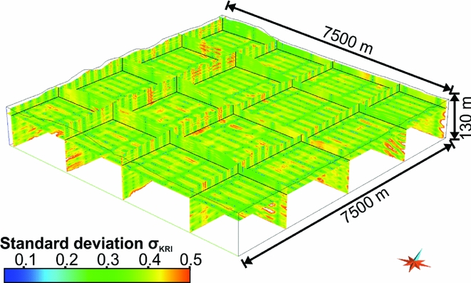
3) Uncertainties may originate from the interpolation method (Pryet et al., Reference Pryet, Ramm, Chilès, Auken, Deffontaines and Violette2011). We focused on uncertainties caused by the kriging interpolation method of the 1D AEM inversion results. A geostatistical uncertainty estimate is provided by the kriging variance σ2 KRI (x, y, z), which depends on the spatial variability of the parameter and the distance to individual data points. This leads to the construction of a 3D grid that contains both resistivity values and their uncertainties (Pryet et al., Reference Pryet, Ramm, Chilès, Auken, Deffontaines and Violette2011). Once the model is built, the analysis of uncertainties between data points (i.e. between flight lines) is expressed by the standard deviation σKRI (Fig. 9). The standard deviation can be used to evaluate the credibility of the interpolated data and to eventually exclude soundings or groups of soundings with high uncertainty and instead emphasise high-quality soundings. A value close to zero indicates high probability and a value close to one indicates low probability of resistivity values. This information can be used to evaluate the relationship between borehole lithology and 3D resistivity data and hence to quantify uncertainties in the depositional architecture.

Fig. 9. 3D view of kriging uncertainty on log-transformed resistivity. Displayed is the kriging standard deviation σKRI from the interpolation process of HFEM data. Low uncertainty traces (dark-blue) indicate the flight lines while the greatest uncertainty is across lines (rather than along lines).
Relationship between lithology and resistivity
Borehole lithology and AEM resistivity were linked with the aim of using resistivity as a proxy for lithology (see: Bosch et al., Reference Bosch, Bakker, Gunnink and Paap2009; Burschil et al., Reference Burschil, Scheer, Kirsch and Wiederhold2012b). The resistivity log from borehole Hl9 (Fig. 10) and sediment descriptions from 487 borehole logs (Fig. 1C) were used to combine these parameters (Fig. 11).

Fig. 10. Seismic section (A), resistivity log (B) and lithology log (C) of borehole Hl9 Wanhoeden (after Besenecker, Reference Besenecker1976). The blue curve shows the measured resistivity log of the borehole, the green curve displays the resistivity log extracted from the 3D HFEM resistivity grid and the red curve displays the projected resistivity log extracted from the 3D HTEM resistivity grid.
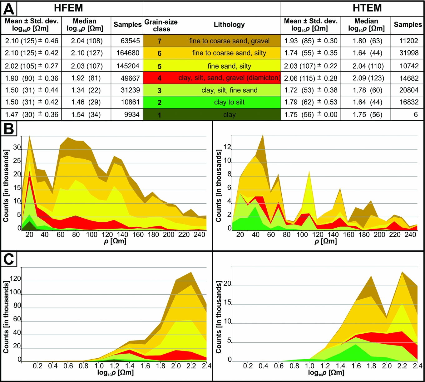
Fig. 11. Grain-size classes and related resistivity histograms extracted from the interpolated 3D HFEM and HTEM resistivity grid. A. Grain-size classes and related resistivity extracted from the interpolated 3D HFEM and HTEM resistivity grid. Shown are mean values, standard deviation, median values and number of counts for common resistivity (logarithmic values). B. Histogram showing resistivity classes of HFEM and HTEM data for each grain-size class as stacked bars (linear scale). C. Histogram showing resistivity classes of HFEM and HTEM data for each grain-size class as stacked bars (logarithmic scale). The absence of resistivity values lower than 1 log10 Ωm indicates that the influence of anthropogenic noise and saltwater can be excluded.
The electrical resistivity of sediments is mainly controlled by the presence of clay minerals, the degree of water saturation and the pore water ion content. According to Archie (Reference Archie1942), resistivity for clay-free sediments is inversely proportional to the pore water ion content. If the specific pore water ion content is known throughout the different geological layers and structures, estimates in lithology variations related to the clay content and type can be obtained. Because saline groundwater is absent in the study area, at least at depths resolved by HFEM (Siemon, Reference Siemon2005), resistivity changes are related to changes in lithology.
The lithologies were divided into seven grain-size classes based on the borehole descriptions. In accordance with data resolution, we determined the representative lithology in each borehole and extracted the corresponding interpolated resistivity at this location from the 3D resistivity grids based on the two different AEM data sets. We accept in this step that the lithology logs within the study area have varying resolutions ranging from 1 cm to 1 m, depending on the drilling method and data collection. This may lead to a discrepancy between the lithology log and the vertical resolution of the 3D AEM resistivity grids, resulting in insufficient resistivity–grain size relationships. To reduce the uncertainty between the lithology logs and resistivity grid we analysed all logs and calculated mean and median resistivity values for each class that allowed derivation of grain size from resistivity (Fig. 11). Grouping the data into resistivity classes and counting the number of occurrences of each lithology resulted in the proportion of occurrences of each grain-size class per resistivity group (Fig. 11). As high resistivity values in the study area often represent dry sediments, we focused on resistivity values up to 250 Ωm.
Integration of the 3D resistivity grids with the 3D geological subsurface model
To test the match between the 3D resistivity grid models (based on 1D inversion results of AEM data) and the 3D geological subsurface model (based on borehole and seismic data), we integrated both into GOCAD (Fig. 3C). To verify the validity and accuracy of data and their integration we followed a mutual comparison between seismic reflector pattern and the corresponding resistivities obtained from the 3D AEM resistivity grids in GOCAD (Figs 4C and D Fig. 5C and D) and related grain-size classes defined from borehole logs to resistivity values derived from the 3D AEM resistivity grid models (Fig. 11).
Adjustment of the 3D geological subsurface model
The GOCAD modelling software has various possibilities to visualise properties such as resistivity values of the 3D grid models to facilitate use and interpretation of data. This includes changes in the colour scale, the selection of given resistivity ranges and voxel volumes. The selection of specific resistivity ranges in the 3D resistivity grid model, in particular, provides a first rough estimate of the three-dimensional geological architecture (Fig. 3D).
In this study, we propose a method for 3D geological modelling of AEM data in which the limitations are jointly considered. The relationship between lithology and resistivity and its corresponding resistivity values was used to adjust the bounding surfaces of the geological framework model. After adjusting the geologic framework the updated 3D geological subsurface models were combined with the 3D HFEM voxel grid. Voxel grids can hold an unlimited number of attributes and different parameters can be added to the grid structure as attributes such as lithology, facies or model uncertainty. The high resolution of the regular voxel model allows the subsurface structure to be maintained. The result is a more reliable reconstruction of the shallow subsurface architecture (Figs 4–7). Nevertheless, internal lithology variations as identified on seismic sections and the heterogeneity of sediments represented by overlapping resistivity ranges often leads to ambiguous lithological interpretation.
Verification of the 3D geological subsurface models by means of HFEM forward modelling
We compared the apparent resistivity values at each frequency of the HFEM survey (Fig. 12A) with the apparent resistivity values derived from the initial 3D geological subsurface model based on borehole and seismic data (Fig. 12B) and the adjusted 3D geological subsurface model derived from the 3D AEM resistivity grids (Fig. 12C). This allowed identification of differences and uncertainties in each data set.

Fig. 12. Apparent resistivity images at different frequencies, corresponding to centroid depths, which increase from left to right. A. Apparent resistivity images of measured HFEM data. B. Apparent resistivity images extracted from the 3D geological subsurface model based on borehole and seismic data. C. Apparent resistivity images extracted from the adjusted 3D geological subsurface model derived from AEM data. D. Apparent resistivity images extracted from the adjusted 3D geological subsurface model derived from AEM data with manually adjusted resistivity values based on lithology log information.
At each HFEM data point the thickness and median resistivity value of each geological unit derived from the different 3D geological subsurface models (Tables 1 and 2) were used to create a 1D resistivity model. For all 1D models, synthetic HFEM data were derived and transformed to apparent resistivity values at each HFEM frequency (Siemon, Reference Siemon2001). To verify the HFEM data, apparent resistivities were used to compare the measured and modelled HFEM data for two reasons: (1) the apparent resistivities are almost always independent of altitude variations of the HFEM system (Siemon et al., Reference Siemon, Christiansen and Auken2009a) and (2) they represent an approximation to the true resistivity distribution in the subsurface. The corresponding depth levels, however, vary as the centroid depth values depend on the penetration depth of the electromagnetic fields.
Results
The depositional architecture of the Cuxhaven tunnel valley and its Neogene host sediments defined by seismic and borehole data analysis
Neogene marine and marginal marine deposits
The Neogene succession is 360 m thick and unconformably overlies open marine to paralic Oligocene deposits (Kuster, Reference Kuster2005). On the basis of previous investigations of the Neogene sedimentary successions (Gramann & Daniels, Reference Gramann and Daniels1988; Odin & Kreuzer, Reference Odin and Kreuzer1988; Gramann, Reference Gramann1988, Reference Gramann1989; Overeem et al., Reference Overeem, Weltje, Bishop-Kay and Kroonenberg2001; Kuster, Reference Kuster2005; Köthe et al., Reference Köthe, Gaedicke and Rüdiger2008; Rumpel et al., Reference Rumpel, Binot, Gabriel, Siemon, Steuer and Wiederhold2009) four seismic units were mapped within the Neogene deposits, each bounded at the base by an unconformity. These seismic units can be correlated to seismic units in the North Sea Basin (Michelsen et al., Reference Michelsen, Thomsen, Danielsen, Heilmann-Clausen, Jordt, Laursen, Graciansky, Hardenbol, Jacquin and Vail1998; Møller et al., Reference Møller, Rasmussen and Clausen2009; Anell et al., Reference Anell, Thybo and Rasmussen2012). The main characteristics of seismic units, including seismic facies, sedimentary facies and mean resistivity values are summarised in Table 1. The overall thickening observed in the westward dip direction of the seismic units is interpreted as an effect of the salt rim syncline subsidence creating accommodation space (cf. Maystrenko et al., Reference Maystrenko, Bayer and Scheck-Wenderoth2005a,Reference Maystrenko, Bayer and Scheck-Wenderothb; Grassmann et al., Reference Grassmann, Cramer, Delisle, Messner and Winsemann2005; Brandes et al., Reference Brandes, Pollok, Schmidt, Riegel, Wilde and Winsemann2012). The deposits consist of fine-grained shelf to marginal marine sediments.
At the end of the Miocene an incised valley formed that was subsequently filled with Pliocene delta deposits, probably indicating a palaeo-course of the River Weser or Elbe (Figs 4, 5 and 6). This is confirmed by the sub-parallel pattern of the lower valley fill onlapping reflector terminations onto the truncation surface observed in seismic lines S1 and S2. This is interpreted as transgressive backstepping (seismic lines S1 and S2; Table 1; Figs 4A and B, and 5A and B; Dalrymple et al., Reference Dalrymple, Zaitlin and Boyd1992). The upper part of the incised-valley fill is characterised in the seismic by mound- and small-scale U-shaped elements, which are interpreted as prograding delta lobes (seismic lines S1 and S2; Figs 4A and B, and 5A and B).
Pleistocene and Holocene deposits
Pleistocene deposits unconformably overly the marginal-marine Neogene sediments and are separated at the base by an erosional surface characterised by two steep-walled tunnel valleys passing laterally into subhorizontal surfaces (Fig. 4A and B). The large tunnel valley is up to 350 m deep and 2 km wide (seismic line S1 and S2, Figs 4A and B, and 5A and B) and has previously been described by Kuster & Meyer (Reference Kuster and Meyer1979), Siemon et al. (Reference Siemon, Stuntebeck, Sengpiel, Röttger, Rehli and Eberle2002, Reference Siemon, Eberle and Binot2004), Gabriel et al. (Reference Gabriel, Kirsch, Siemon and Wiederhold2003), Siemon (Reference Siemon2005), Wiederhold et al. (Reference Wiederhold, Binot and Kessels2005a), Gabriel (Reference Gabriel2006), Rumpel et al. (Reference Rumpel, Binot, Gabriel, Siemon, Steuer and Wiederhold2009) and BurVal Working Group (2009). The smaller tunnel valley in the east is up to 200 m deep and 1 km wide (seismic line S1, Fig. 4A and B). In total, eight seismic subunits were mapped within these tunnel valleys and the marginal areas (U5.1–U5.8; cf. Table 2; Figs 4B and 5B). The main characteristics of seismic subunits, including seismic facies, sedimentary facies and mean resistivity values, are summarised in Table 2.
The dimension, geometry, internal reflector pattern and sedimentary fill of the troughs correspond well to Pleistocene tunnel-valley systems described from northern Germany (Ehlers & Linke, Reference Ehlers and Linke1989; Stackebrandt, Reference Stackebrandt2009; Lang et al., Reference Lang, Winsemann, Steinmetz, Polom, Pollok, Böhner, Serangeli, Brandes, Hampel and Winghart2012; Janszen et al., Reference Janszen, Moreau, Moscariello, Ehlers and Kröger2013), Denmark (Jørgensen & Sandersen, Reference Jørgensen and Sandersen2009), the Netherlands (Kluiving et al., Reference Kluiving, Bosch, Ebbing, Mesdag and Westerhoff2003) and the North Sea Basin (Wingfield, Reference Wingfield1990; Huuse & Lykke-Andersen, Reference Huuse and Lykke-Andersen2000; Praeg, Reference Praeg2003; Lutz et al., Reference Lutz, Kalka, Gaedicke, Reinhardt and Winsemann2009; Kehew et al., Reference Kehew, Piotrowski and Jørgensen2012; Moreau et al., Reference Moreau, Huuse, Janszen, van der Vegt, Gibbard, Moscariello, Huuse, Redfern, Le Heron, Dixon, Moscariello and Craig2012). The basal fill consists of Elsterian meltwater deposits overlain by glaciolacustrine deposits of the Lauenburg Clay Complex. These deposits are unconformably overlain by marine Holsteinian interglacial deposits. Saalian meltwater deposits and till cover the entire study area and unconformably overly the Neogene, Elsterian and Holsteinian deposits (Table 2; Figs 4A and B, and 5A and B).
Integration of the resistivity grid model and the geological subsurface model
Comparison of borehole resistivity logs with model resistivity data
The borehole Hl9 Wanhoeden penetrates the western marginal tunnel-valley fill (cf. Figs 1C and 4B). The lowermost fill consists of Elsterian glaciolacustrine fine- to medium-grained sand and silt alternations of the Lower Lauenburg Clay Complex (U5.2–5.4). This succession is overlain by the Upper Lauenburg Clay Complex, which consists of clay, silt and fine-grained sand alternations (U5.5–5.6) and marine Holsteinian interglacial deposits (U5.7; Figs 4B and 10). The resistivity log of borehole Hl9 displays strong resistivity variations, which can be correlated with the alternation of clay- and sand-rich beds (Fig. 10). The 3D resistivity grid model based on 1D HFEM inversion results displays a similar resistivity log as the one in the borehole and thus a good lithological match. The upper bounding surface of the Upper Lauenburg Clay Complex and the marine interglacial Holsteinian clay can also be identified on the 3D resistivity grid model (Fig. 10). The interpolated 3D resistivity grid model based on 1D HTEM inversion results, however, reveals only one conductor. While the Upper Lauenburg Clay Complex is nearly fully imaged, the interglacial marine Holsteinian clay is not well defined, which may be caused by the limited resolution of the transient electromagnetic (TEM) method. The highly conductive sediments of the Upper Lauenburg Clay Complex lead to a reduced penetration of the electromagnetic fields and hence resistivities of the sediments below the Upper Lauenburg Clay Complex are not detectable with the transmitter moments used in this survey.
An important difference between resistivity values of the measured resistivity log of borehole Hl9 and the extracted values from the 3D resistivity grid models based on 1D AEM inversion results is the amplitude of high resistivity values, which is considerably lower in the 3D resistivity grid models (Fig. 10). This difference can be explained by the applied AEM methods, which are more sensitive to conductive sediments (Steuer et al., Reference Steuer, Siemon and Auken2009). In addition, the AEM system predominantly generates horizontal currents, whereas electromagnetic borehole systems use vertical currents for measuring the log resistivity. Sediment anisotropy as well as scaling effects has also to be taken into account.
Relationship between borehole lithology logs and AEM model resistivities
Our analysis shows that resistivity generally increases with grain size and permeability, as also shown by Burschil et al. (Reference Burschil, Scheer, Kirsch and Wiederhold2012b) and Klimke et al. (Reference Klimke, Wiederhold, Winsemann, Ertl and Elbracht2013) for HTEM data. However, there are substantial differences between the borehole lithology and resistivity values derived from the two interpolated 3D AEM resistivity grids (Fig. 11). The 3D HFEM resistivity grid indicates that clay (grain-size class 1) has an average resistivity of 30 Ωm in the study area. This value corresponds to previous results of AEM data commonly reported in the literature for clay (Burschil et al., Reference Burschil, Scheer, Kirsch and Wiederhold2012b; Klimke et al., Reference Klimke, Wiederhold, Winsemann, Ertl and Elbracht2013). In comparison to borehole resistivity (commonly between 5 and 20 Ωm) the 3D HFEM resistivity value is slightly to high and may be caused (1) by a certain silt and sand content or (2) by the limited resolution of the HFEM method providing an over- or underestimated thickness or merging of lithological units. The average resistivity value for deposits mainly consisting of clay to silt is 31 Ωm (grain-size class 2), for clay- and silt-rich fine sand is 31 Ωm (grain-size class 3), for diamicton is 80 Ωm (grain-size class 4), for fine sand is 105 Ωm (grain-size class 5), for silt-rich fine to coarse sand is 125 Ωm (grain-size class 6) and for fine to coarse sand with gravel is 125 Ωm (grain-size class 7).
The relationship between borehole lithology and resistivity data extracted from the grid based on 1D HTEM inversion results does not allow the lithology to be clearly defined in 3D (Fig. 11). The average resistivity value for clay from our data set (grain-size class 1) is 56 Ωm and may be skewed due to the small sample number. The average resistivity value for deposits mainly consisting of clay to silt is 62 Ωm (grain-size class 2), for clay- and silt-rich fine sand is 53 Ωm (grain-size class 3), for diamicton is 115 Ωm (grain-size class 4), for fine sand is 107 Ωm (grain-size class 5), for silt-rich fine to coarse sand is 55 Ωm (grain-size class 6) and for fine to coarse sand with gravel is 85 Ωm (grain-size class 7).
The histograms for both resistivity data sets (see Fig. 11) demonstrate that the measured values for sand are higher than for deposits with certain clay content. However, overlapping resistivity values for sand-dominated sediments and deposits with clay content are generally found to have a lower resistivity range, especially for the HTEM resistivity data set. The coarser-grained sediments (grain-size class 4 to 7) have a wide variety of resistivity values and seem too low, especially for the HTEM data set. Fig. 11 displays these large resistivity ranges. The variance in values is interpreted to result from the mixed lithological components, the limited resolution of the AEM system and the less distinctive imaging of low-conductive sediments.
The larger overlaps of HTEM resistivity values can be explained as an effect of restricted HTEM data coverage and the projection of interpolated resistivity values onto the borehole locations. Similar HTEM resistivity values were found at the island of Föhr (Burschil et al., Reference Burschil, Wiederhold and Auken2012a,Reference Burschil, Scheer, Kirsch and Wiederholdb) and for the region of Quakenbrück, southwestern Lower Saxony (Klimke et al., Reference Klimke, Wiederhold, Winsemann, Ertl and Elbracht2013). Nonetheless, discrimination of different lithologies with a wide range of resistivity values is possible by integrating with other data sets, for example borehole or seismic reflection data.
Correlation of the HFEM resistivity model with the geological model
Neogene marine and marginal marine deposits
At depths between 10 and 120 m the spatial resistivity pattern is characterised by an elongated structure with gradual large-scale variations (100–300 m) of medium to high resistivity values that indicate the heterogeneous infill of the Late Miocene incised valley (seismic unit U4; Figs 4C and 5C). A positive correlation with the hummocky seismic reflector pattern and borehole lithology indicates that the resistivity pattern images grain-size variations of vertically and laterally stacked delta lobes (cf. Figs 4C and 5C).
Pleistocene deposits
The difference in lithology between the fine-grained glacigenic Pleistocene deposits of the upper tunnel-valley fill and the coarser-grained Neogene marginal-marine sediments is expressed as a distinct resistivity contrast, which can be clearly traced in depth (Figs 4C, 5C and 6B).
The margin of the Cuxhaven tunnel valley is indicated by a gradual shift from low to medium resistivity values of Pleistocene deposits (seismic subunits U5.5, U5.6 and U5.7; Figs 4C, 5C, 6B and 7B) to higher resistivity values of the Pliocene host sediments (seismic unit U4; Figs 4C, 5C, 6B and 7B). The resistivity pattern of the HFEM model enables a good 3D imaging of the internal tunnel-valley fill. Large- and small-scale, elongated, wedge-shaped or lens-shaped variations in the resistivity pattern can be correlated with major seismic units and smaller-scale architectural elements, such as individual channels (cf. Fig. 4C: U5.7 between 3800 and 4000 m) and lobes (cf. Fig. 4C: U5.6 and U5.7 between 3600 and 3700 m).
The overall tabular geometry of the glaciolacustrine deposits of the Lauenburg Clay Complex (seismic subunit U5.6) and the marine Holsteinian interglacial deposits (seismic subunit U5.7) are both characterised by low resistivity values in the tunnel-valley centre (Figs 4C, 5C, 6B and 7B) and gradually into higher resistivity values towards the tunnel-valley margin. The higher resistivity values towards the tunnel-valley margin have been interpreted to be the result of bleeding of higher resistivity values from the neighbouring Pliocene sediments. Alternatively, they could be interpreted as an indicator for coarse-grained material (e.g. delta foresets at the margin of the tunnel valley in Fig. 5C: U5.2 and U5.4 between 700 and 800 m; in Fig. 4C: U5.5 at 4300 m and U5.6 at 4500 m). The comparison with lithology data from boreholes proves that the Lauenburg Clay Complex (seismic subunit U5.6) and the marine Holsteinian deposits (seismic subunit U5.7) are approximately imaged at the correct depths. The HFEM resistivity pattern, however, does not image a distinct boundary between the glaciolacustrine Lauenburg Clay Complex and the marine Holsteinian interglacial deposits due to their similar grain sizes.
Within the tunnel-valley centre thick conductive fine-grained beds of the Lauenburg Clay Complex limit the penetration depth of the HFEM system, leading to a decrease in resolution and a less distinct resistivity pattern of underlying fine- to medium-grained sand (cf. Fig. 5C, seismic subunit U5.5 in seismic line S2). Similar results have also been observed by Steuer et al. (Reference Steuer, Siemon and Auken2009).
In the eastern part of the study area lower resistivity values in HFEM data are identified, which differ from the Neogene host sediments. Its geometry and resistivity values suggest a smaller-scale tunnel valley and probably indicate a fill of fine-grained glaciolacustrine (Lauenburg Clay Complex) and/or interglacial marine (Holsteinian) deposits (Fig. 4C). The low resistivity contrast between this tunnel-valley fill and the Neogene host sediments probably indicates relatively similar grain sizes, but this remains speculative because no borehole log control is available.
In the uppermost part of the Pleistocene succession between 0 and 10 m depth (seismic subunit U5.8; Figs 4C and 5C) a distinct shift from low to very high resistivity values indicates a strong increase in electrical resistivity. This resistivity shift is interpreted to represent the transition between water saturated and unsaturated sediments – it represents the groundwater table contact. This strong resistivity contrast allows the detection of the groundwater table within a range of approximately 2 m and clearly outlines the Hohe Lieth ridge as the most important groundwater recharge area, which has also been documented by Blindow & Balke (Reference Blindow and Balke2005).
Correlation of the HTEM resistivity model with the geological model
Neogene marginal-marine deposits
At depths between 180 and 150 m (seismic unit U3) the resistivity pattern is characterised by a sharp contrast from low to medium resistivity values (Figs 4D, 5D, 6B and 7B). This upward increase in resistivity is interpreted as an abrupt facies change from finer-grained shelf deposits to coarser-grained shoreface deposits, which is also recorded in borehole data (Kuster, Reference Kuster2005) and might be related to the rapid onset of progradation during the highstand systems tract.
Correlation of the resistivity pattern with borehole data indicates that the low resistivity values link to marine Early Tortonian clays (seismic unit U3). At depths between 120 and 80 m, large-scale, lateral variations of low to medium resistivity values, parallel to seismic reflections, can be identified. Altogether, resistivity contrast and seismic pattern, characterised by strong reflectivity contrasts, are interpreted to result from grain-size variations, which probably indicate the Tortonian to Messinian storm-dominated shoreface deposits (seismic unit U3; Table 1; Figs 4D and 5D; Walker & Plint, Reference Walker, Plint, Walker and James1992; Catuneanu, Reference Catuneanu2002; Kuster, Reference Kuster2005; Catuneanu et al., Reference Catuneanu, Galloway, Kendall, Miall, Posamentier, Strasser and Tucker2011). Gradual vertical transitions from low to high resistivity values within the upper Neogene unit (seismic unit U4; Figs 4D and 5D) correspond to borehole lithology data with an overall coarsening-upward trend are interpreted as prograding delta lobes (e.g. Dalrymple et al., Reference Dalrymple, Zaitlin and Boyd1992; Plink-Björklund, Reference Plink-Björklund, Hampson, Steel, Burgess and Dalrymple2008). This interpretation is further supported by the seismic pattern of lobate units (Figs 4A and B and 5A and B).
Pleistocene deposits
The lithology contrast between the fine-grained glacigenic Pleistocene deposits at the base and the underlying coarser-grained Neogene marginal-marine sediments is expressed as a distinct change in resistivity, which can be clearly traced in the shallow subsurface between 20 and 30 m depth and corresponds to the lower boundary of seismic unit U5 (Figs 4D and 5D). The tunnel-valley margin can be identified in borehole data, but in the deeper subsurface is not clearly imaged by the HTEM resistivity data. At the tunnel-valley margin the resistivity resembles that of the adjacent Neogene host sediments and therefore its boundary may not be as easily distinguished (Figs 4D, 5D, 6C and 7C). The inability for the HTEM data to have contrasting resistivity values to define the tunnel-valley boundary is probably caused by the large lateral footprint of the HTEM system, the inversion approach (SCI) and the kriging method, which leads to a smooth transition between individual resistivity values.
The upper Cuxhaven tunnel-valley fill is characterised by different vertically stacked resistivity patterns. The highly conductive sediments of the Lauenburg Clay Complex lead to a reduced penetration of the EM field and the resistivity of the sediments below are not detectable with the transmitter moments used in this survey. This suggests that the medium resistivity values imaged at depths between 160 and 80 m do not necessarily show the true resistivities of Pleistocene sand within the tunnel valley recorded in borehole data (seismic subunits U5.1 to U5.4; Figs 4D and 5D). However, the distinct shift towards higher resistivity values in the unit below the highly conductive sediments of the Lauenburg Clay Complex probably indicates coarser-grained deposits of seismic subunit U5.5 (Figs 4D and 5D). At depths between 80 and 10 m low resistivity values can be correlated with fine-grained glaciolacustrine sediments of the Lauenburg Clay Complex and interglacial Holsteinian deposits (seismic subunit U5.6 and U5.7; Figs 4D and 5D). The comparison of the resistivity data with the borehole logs and seismic data (Fig. 5B) indicates that resistivity changes reflect lithological changes.
Verification of apparent resistivity values extracted from the 3D subsurface models
The comparison of the apparent resistivity values derived from the HFEM data (Fig. 12A), the initial geological subsurface model based on borehole and seismic data (Fig. 12B), and the adjusted geological subsurface model derived from the 3D AEM resistivity grids (Fig. 12C) generally show a relationship indicating that both geological models are able to explain the principal resistvity distribution at several HFEM frequencies. The apparent resistivity images of the initial 3D geological subsurface model show a relatively sharp resistivity contrast between the Pleistocene tunnel valley and the adjacent Neogene deposits (Fig. 12B), particularly at the lower frequencies (at greater depths) defining a simple tunnel-valley geometry with a low sinuosity. The apparent resistivity map derived from the initial 3D geological subsurface model (Fig. 12B), however, does not image the tunnel-valley fill at the highest frequency (at shallow depths). The difference between the apparent resistivity images can be explained by the limited coverage of borehole and seismic data, which leads to restricted information about the subsurface architecture. The apparent resistivity images of the adjusted 3D geological subsurface model derived from the 3D AEM resistivity grids (Fig. 12C) show a more complex tunnel-valley geometry characterised by a higher sinuosity and smaller-scale variations of the resistivity pattern. This more complex interpretation of the tunnel valley can be better aligned with the apparent resistivity images of HFEM data (Fig. 12A) and the lithology variations recorded by borehole data. Nevertheless, uncertainties remain and are caused by the decreasing resolution with depth, which may lead to less contrast in the resistivity images. This is especially apparent at the lowest frequency, whereby the resistivity images are influenced by underlying sediments. This often leads to the bottom layer of the 1D inversion models being represented by incorrect resistivity values. To reduce this problem we manually adjusted the resistivity values of bottom units in the adjusted 3D geological subsurface model derived from the 3D AEM resistivity grids based on lithology information (i.e. in particular the resistivity value for the lower part of unit U3 representing clay and silt was reduced by a factor of about 2; cf. Table 1). The resistivities of the valley infill were adjusted if the calculated mean values were misleading for the sediment type (i.e. too high resistivities attributed to clay and silt units were reduced, e.g. seismic subunit U5.3, and too low resistivities attributed to sandy units were increased, e.g. seismic subunits U5.1 and U5.4; cf. Table 2). Some other values were rounded.
We re-calculated the apparent resistivity values after correction (Fig. 12D). These resistivity images better represent the subsurface architecture and are closer to the apparent resistivity maps represented in the HFEM data, i.e. the adjusted geological model better explains the HFEM data. Nevertheless, differences in the images of the apparent resistivity patterns remain. This is caused by a too low resolution of the 3D geological subsurface model, which does not represent detailed sediment variability, and incorrectly estimated resistivities attributed to the geological units. A good example of this effect is the area of the smaller tunnel valley in the eastern part of the study area (Fig. 12D), where the clay and silt deposits (lower part of U3) are obviously thinner or/and resistive, and the central part of the valley fill U5.5* was estimated as too broad and too conductive. On the other hand, the low apparent resistivities in the northwest of the study area, which occur particularly at low frequencies, are caused by anthropogenic sources (airport Cuxhaven/Nordholz).
Discussion
Our results show that AEM data provide excellent opportunities to map the subsurface geology as previously demonstrated by, for example, Newman et al. (Reference Newman, Hohmann and Anderson1986), Jordan & Siemon (Reference Jordan and Siemon2002), Danielsen et al. (Reference Danielsen, Auken, Jørgensen, Søndergård and Sørensen2003), Jørgensen et al. (Reference Jørgensen, Sandersen and Auken2003b, Reference Jørgensen, Sandersen, Auken, Lykke-Andersen and Sørensen2013), Auken & Christiansen (Reference Auken and Christiansen2004), Auken et al. (Reference Auken, Christiansen, Jacobsen and Sorensen2008), Viezzoli et al. (Reference Viezzoli, Christiansen, Auken and Sørensen2008), Bosch et al. (Reference Bosch, Bakker, Gunnink and Paap2009), Christensen et al. (Reference Christensen, Reid and Halkjær2009), Klimke et al. (Reference Klimke, Wiederhold, Winsemann, Ertl and Elbracht2013) and Gunnink & Siemon (Reference Gunnink and Siemon2014). A good relationship between resistivity values and lithology enables the 3D imaging of the subsurface architecture. This allows a hitherto unseen amount of geological detail using AEM data in areas of low borehole coverage. This approach provides an advanced 3D geological model of the study area with new geological insights. Although the presented approach is more time-consuming than an automated approach that relies on statistics-based methods (Bosch et al., Reference Bosch, Bakker, Gunnink and Paap2009; Gunnink et al., Reference Gunnink, Bosch, Siemon, Roth and Auken2012), the end results compensate for the limitations of the AEM method.
Geological and geophysical models and their interpretations contain limitations and uncertainties resulting from limitations in the input information (Ross et al., Reference Ross, Parent and Lefebvre2005). Several studies focussed on the analysis of such limitations and uncertainties in order to minimise risk, e.g. exploration risks (Bárdossy & Fodor, Reference Bárdossy and Fodor2001; Pryet et al., Reference Pryet, Ramm, Chilès, Auken, Deffontaines and Violette2011; Wellmann & Regenauer-Lieb, Reference Wellmann and Regenauer-Lieb2012; Jørgensen et al., Reference Jørgensen, Rønde Møller, Nebel, Jensen, Christiansen and Sandersen2013). Uncertainties and limitations in the integrated interpretation of AEM and ground-based data are mainly caused by the restricted availability and limited vertical and lateral resolution of data (e.g. boreholes, seismic sections, airborne surveys), modelling errors caused by a misinterpretation of geophysical, lithological and hydrogeological properties, anthropogenic noise effects, missing software interoperability (Mann, Reference Mann, Davis and Herzfeld1993; Bárdossy & Fodor, Reference Bárdossy and Fodor2001; Ross et al., Reference Ross, Parent and Lefebvre2005; Pryet et al., Reference Pryet, Ramm, Chilès, Auken, Deffontaines and Violette2011) and irreducible, input-geology related, uncertainty. In general there are several limitations in the interpretation caused by the applied AEM systems and the chosen data analysis.
The penetration depth and resolution of both AEM systems used is controlled by lithology and their conductivity. The penetration depth is limited to approximately 100 m for HFEM and 250 m for HTEM, and both systems are subject to decreasing resolution capability with depth and require an increasing thickness/depth ratio for the detection of varying depositional units (Jørgensen et al., Reference Jørgensen, Sandersen and Auken2003b, Reference Jørgensen, Sandersen, Auken, Lykke-Andersen and Sørensen2005; Høyer et al., Reference Høyer, Lykke-Andersen, Jørgensen and Auken2011). Because of the wide range of lithologies a significant uncertainty remains in the final interpretation of the resistivity pattern. Hence, thin-bedded sedimentary units are only resolved if their corresponding conductance, i.e. the ratio of thickness and resistivity, is sufficiently high. Otherwise they will be merged into a single unit with an average resistivity (Jørgensen et al., Reference Jørgensen, Sandersen and Auken2003b, Reference Jørgensen, Sandersen, Auken, Lykke-Andersen and Sørensen2005), which results in a limited resistivity resolution. The limitations in lateral and vertical resolution can lead to incorrect interpretations of thin-bedded sand/mud couplets, smaller-scale architectural elements and bounding surfaces, as has been also shown by, for example, Jørgensen et al. (Reference Jørgensen, Lykke-Andersen, Sandersen, Auken and Nørmark2003a, Reference Jørgensen, Sandersen, Auken, Lykke-Andersen and Sørensen2005), Viezzoli et al. (Reference Viezzoli, Christiansen, Auken and Sørensen2008), Christensen et al. (Reference Christensen, Reid and Halkjær2009) and Klimke et al. (Reference Klimke, Wiederhold, Winsemann, Ertl and Elbracht2013). This problem is distinctly seen in our study area in the Pleistocene tunnel valley and Late Miocene incised valley. The Saalian till at 20 m depth with a thickness between 5 and 10 m and a wide resistivity range (cf. Fig. 11) could not be differentiated from the surrounding lithology and is beyond the possible AEM resolution. The Pleistocene tunnel-valley margins and the Late Miocene incised-valley margin could not be detected because of a low resistivity contrast to the adjacent Neogene host sediments.
For our study only an existing 1D AEM inversion data set (from 2002) was available, in which noise effects were not significantly minimised, as commonly applied for new data sets (e.g. Tølbøll, Reference Tølbøll2007; Siemon et al., Reference Siemon, Steuer, Ullmann, Vasterling and Voß2011). However, the noise effects of anthropogenic structures and soundings in the airborne electromagnetic data can hinder a proper geological interpretation, e.g. the airport Cuxhaven/Nordholz located in the northwest of the study area. In the case of the study area anthropogenic noise effects cause unrealistic low resistive oscillations, which conically increase downwards.
We used a geostatistical approach to analyse and interpolate the 1D AEM inversion results to create a continuous 3D resistivity subsurface grid. We used ordinary kriging, and in contrast to Pryet et al. (Reference Pryet, Ramm, Chilès, Auken, Deffontaines and Violette2011) we discarded the layered approach used in the 1D inversion of AEM data, leading to a smoothing effect between previously defined layer boundaries. The advantage of this method is that the kriging algorithm indicates the most likely resistivity value at each grid cell. The result is an effectively smoothed resistivity grid, leading to a significant improved geological interpretation of continuous lithofacies. However, a loss of heterogeneity that is probably observed in the subsurface by AEM has to be taken into account. If the aim is to generate fluid-flow models it is important to preserve the porosity and permeability of varying lithologies as these strongly determine fluid-flow behaviour through porous media (e.g. Koltermann & Gorelick, Reference Koltermann and Gorelick1996; Janszen, Reference Janszen2012). It is therefore preferred to base fluid-flow simulations on grids that are interpolated using algorithms that are able to preserve the heterogeneity, such as modified kriging methods like the sequential indicator simulation used by Venteris (Reference Venteris2007), Bosch et al. (Reference Bosch, Bakker, Gunnink and Paap2009) and Janszen (Reference Janszen2012).
A common limitation of the presented workflow is the high degree of subjectivity that causes uncertainties that are hard to evaluate. To test the reliability of the 3D geological subsurface model and evaluate uncertainty, we followed a new approach to derive synthetic HFEM data from the geological model results based on a relationship of calculated or assumed geological units and resistivities. The comparison between corresponding apparent resistivity images of the subsurface based on AEM field measurements and 3D geological models leads to the identification of uncertainties and limitations of 1D AEM inversion and vice versa. The results of such analyses will offer the advantage of using a priori information to improve the inversion of AEM data, comparable to investigations made by, for example, Zhdanov (Reference Zhdanov2010) and Gunnink et al. (Reference Gunnink, Bosch, Siemon, Roth and Auken2012).
Conclusions
Resistivity data derived from AEM surveys can provide a fast and efficient overview mapping of the shallow subsurface geology. A methodology for the interpretation, analysis and imaging of resistivity data gained by AEM surveys, based on 3D modelling approaches, was developed. We used 1D HFEM and HTEM inversion results and applied a 3D resistivity gridding procedure based on geostatistical analyses and interpolation techniques to create continuous resistivity models of the subsurface. Subsequently, we integrated results of seismic facies and borehole lithology analysis to construct a combined 3D geological subsurface model and to reduce uncertainties. This approach allows for an improved interpretation of AEM data and imaging of the 3D subsurface architecture, if the relationship between lithology and resistivity was known and the site was only slightly influenced by noise effects (e.g. infrastructural networks, settlements).
The 3D resistivity models clearly allow discrimination between different lithologies and enable the detection of Cenozoic sequence boundaries and larger-scale architectural elements such as incised valleys and subglacial tunnel valleys. Variations in the resistivity pattern allowed the detection of individual delta lobes and smaller-scale channels as well as lateral and vertical grain-size variations. In the Neogene succession a low resistive pattern can be correlated with Tortonian and Messinian marine clays. The lowest values probably correspond with the zone of maximum flooding. From seismic interpretation we conclude that at the end of the Miocene an incised valley formed as a response to a major sea-level fall that subsequently became filled with Pliocene-delta deposits, probably indicating the palaeo-course of the Rivers Weser or Elbe. The resistivity models clearly image the outline of the Pleistocene tunnel valleys. The unconsolidated fill of the Late Miocene to Pliocene incised valley probably formed a preferred pathway for the Pleistocene meltwater flows, favouring the incision of a subglacial tunnel valley. Based on the 3D HFEM resistivity grid the fills of the tunnel valleys could be imaged in much more detail in comparison to previously published descriptions based on the 2D seismic sections and 2D AEM profiles and maps. The applied approaches and results show a reliable methodology, especially for future investigations of similar geological settings.
Acknowledgements
The AIDA project is part of the joint research program of GEOTECHNOLOGIEN. Financial support is gratefully acknowledged from the German Federal Ministry of Education and Research (BMBF) grant 03G0735. We thank two anonymous reviewers for very careful and constructive reviews, which helped to improve the manuscript. Many thanks are due to Hajo Götze and Peter Menzel for discussion, and Guillaume Martelet for helpful comments on an earlier version of the manuscript and Ariana Osman for discussion and improving the English. We are grateful to the State Authority for Mining, Energy and Geology (LBEG) for providing borehole data, to Fugro for providing the GeODin software and Paradigm for GOCAD software support.


